Fidelity of Quantum Interferometers

Abstract

For a generic interferometer, the conditional probability density distribution, $p(\phi|m)$, for the phase $\phi$ given measurement outcome $m$, will generally have multiple peaks. Therefore, the phase sensitivity of an interferometer cannot be adequately characterized by the standard deviation, such as $\Delta\phi\sim 1/\sqrt{N}$ (the standard limit), or $\Delta\phi\sim 1/N$ (the Heisenberg limit). We propose an alternative measure of phase sensitivity–the fidelity of an interferometer–defined as the Shannon mutual information between the phase shift $\phi$ and the measurement outcomes $m$. As an example application of interferometer fidelity, we consider a generic optical Mach-Zehnder interferometer, used as a sensor of a classical field. We find the surprising result that an entangled N00N state input leads to a lower fidelity than a Fock state input, for the same photon number.

Introduction. Phase sensitivity of interferometers has been a topic of research for many years because of interest in the fundamental limitations of measurement Godun2001 ; Giovannetti2006 , gravitational-wave detectionThorne1980 , and optical Chow1985 ; Bertocchi2006 , atom Zimmer2004 , and Bose-Einstein condensate(BEC)-based gyroscopesGupta2005 ; Wang2005 ; Tolstikhin2005 . Recently, applications to sensors are being exploredDidomenico2004 ; Kapale2005 .   The phase sensitivity of interferometers is believed to be limited by quantum fluctuationsCaves1981 , and the phase sensitivity of various interferometers has been explored for different types of input states, such as squeezed statesCaves1981 ; Bondurant1984 , and number statesYurkePRL1986 ; YurkePRA1986 ; Yuen1986 ; Holland1993 ; Dowling1998 ; Kim1998 ; Pooser2004 ; Pezze2005 ; Pezze2006 . In all the above cases, the phase sensitivity $\Delta\phi$ has been discussed in terms of two limits, known as the standard limit, $\Delta\phi_{SL}=$ $1/\sqrt{N}$, and the Heisenberg limitHeisenberg1927 , $\Delta\phi_{HL}=$ $1/N$, where $N$ is the number of particles that enter the interferometer during each measurement cycle. These arguments are based on results of standard estimation theoryHelstrom1976 which connects an ensemble of measurement outcomes, $m_{i}$, $i=1,2,\cdots,M$, with corresponding phases, $\phi_{i}$, through a theoretical relation $m=m(\phi)$. An example of the theoretical relation associated with some quantum observable is $m(\phi)=\langle\phi|\widehat{m}|\phi\rangle$, where the state is parameterized by a single parameter $\phi$. Standard estimation theory predicts that the standard deviation, $\Delta\phi$, of the probability distribution for the phase $\phi$, is related to the standard deviation in the measurements, $\Delta m$, by Helstrom1976

$$\Delta\phi=\left|\frac{dm(\overline{\phi})}{d\phi}\right|^{-1}\,\Delta m.$$ (1)

Equation (1) assumes that there is a single peak in the phase probability density distribution $p(\phi)$, whose width can be characterized by the standard deviation $\Delta\phi$.  In general, a Bayesian analysis of measurement outcomes $m$ for an interferometer can lead to a conditional probability density distribution for the phase, $p(\phi|m)$, that has multiple peaks. Indeed, multiple peaks have been observed by Pezze and Smerzi Pezze2005 ; Pezze2006 in the context of interferometry described by angular momentum algebra YurkePRA1986 ; Kim1998 . Therefore, the standard deviation $\Delta\phi$ is not an adequate metric to characterize the phase sensitivity of an interferometer when multiple peaks are present in the phase probability distribution.

In this Letter, we propose to characterize the phase sensitivity of an interferometer by an alternative metric—the fidelity—which is the Shannon mutual information Shannon1948 ; NielsenChaung2000 , $H(\Phi\colon\!M)$, between the phase shift $\phi$ and the measurement outcomes, $m$. As an example, we consider the specific case of an optical Mach-Zehnder interferometer in a sensor configuration, see Figure 1. We use an exact Bayesian analysis to compute the conditional probability density distribution for the phase $\phi$, $p(\phi|m)$, and we find that multiple peaks exist. We compute the Shannon mutual information, $H(\Phi\colon\!M)$, for two types of input states, Fock states and N00N states, which have been of great interest Kapale2005 ; Mitchell2004 . We find that the fidelity associated with the Fock state input is greater than for N00N state input.

Phase Sensitivity. A quantum interferometer can act as a sensor of an external field $F$. A quantum state $|\Psi_{in}\rangle$ is input into the interferometer and, through an interaction Hamiltonian $H_{I}(F)$, the state interacts with an external classical field $F$, leading to a phase-shifted output state $\ |\Psi(F)\rangle\,\$that is parameterized by the field $F$.  We assume that a single parameter, the phase shift $\phi$, is sufficient to describe the physics of the interaction process.  A general description of such a sensor can then be given in terms of the scattering matrix, $S_{ij}(\phi)$, that connects the $N_{p}$ input-mode field operators $\widehat{a}_{i}$  to the $N_{p}$ output-mode field operators $\widehat{b}_{i}$,

$$\widehat{b}_{i}=\sum_{j=1}^{N_{p}}S_{ij}(\phi)\,\widehat{a}_{j},$$ (2)

where $i,j=1,2,\cdots,N_{p}$ and $\phi$ is the phase shift of the scattered (output) state.  The field $F$ leads to a phase shift $\phi$ of the scattered state, whose detailed relation is determined by the interaction Hamiltonian $H_{I}(F)$, which we do not consider any further here.  The input state evolves through the interferometer according to the unitary time-evolution operator,  $\widehat{U}(\phi)$, which relates the input state at $t=-\,\infty\$to the output state at $t=+\,\infty$,

$$|\Psi_{out}\rangle\,=\,\ \widehat{U}(\phi)\,|\Psi_{in}\rangle.$$ (3)

Measurements are described by a set of Positive Operator-Valued Measure (POVM) operators, $\{\widehat{E}_{1},\widehat{E}_{2},\cdots,\widehat{E}_{N_{m}}\}$, where each operator  $\widehat{E}_{m}$ corresponds to a measurement outcome $m$. The conditional probability of a given measurement outcome $m$ for a given phase shift $\phi$, is the expectation value  $P(m|\phi)=\langle\Psi_{in}|\widehat{E}_{m}(\phi)|\Psi_{in}\rangle$, where the Heisenberg operators $\widehat{E}_{m}(\phi)$ evolve in time and the states are constant. From Bayes’ rule, we find the conditional probability density, $p(\phi|m)$, for the phase shift $\phi$ for a given measurement outcome $m$ is

$$p(\phi|m)=\frac{P(m|\phi)}{\int_{-\pi}^{+\pi}P(m|\phi^{\prime})\,\,d\phi^{\prime}},$$ (4)

where we have assumed a uniform a priori probability density for the phase shift $\phi$.

In order to have a good sensor, the distribution $p(\phi|m)$ should have a narrow peak that is centered about some value of the phase, for each measurement outcome $m$. The phase sensitivity of an interferometer, or quantum interferometric sensor, is usually taken to be the width of the single peak of the probability density $p(\phi|m)$.

A careful analysis of the probabilities $P(m|\phi)$ as functions of the scattering matrix $S_{ij}(\phi)$ shows that in general the probabilities $P(m|\phi)$ are oscillatory functions of $\phi$. Consequently, the probability density for the phase, $p(\phi|m)$, will have multiple peaks. The physics responsible for this is due to the mutual symmetry of the quantum state and the measuring apparatus (described by operators  $\widehat{E}_{m}(\phi)$).

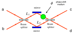
Figure 1: A Mach-Zehnder interferometer is shown consisting of two 50-50 beam splitters and two mirrors. The two input ports and two output ports are shown along with a medium that induces the phase shift $\phi$.  

Since the probability density $p(\phi|m)$ has multiple peaks, the standard deviation $\Delta\phi$ is not an adequate measure of the interferometer’s phase sensitivity.

We propose a new metric for interferometer phase sensitivity–the fidelity–defined as the Shannon mutual information between the set of possible phase values $\phi$, and the possible measurement outcomes $m$. For convenience, we discretize the phase shift into values $\phi_{k}=\pi k/N_{\phi}$, for $k=\pm 1,\pm 2,\cdots\pm,N_{\phi}$, and consider the mutual information between the $2N_{\phi}$ dimensional alphabet of input phases, $\phi_{k}$, and the $N_{m}$-dimensional alphabet of output measurement outcomes, $m=0,1,2,\cdots,N_{m}$. In the limit $N_{\phi}\rightarrow\infty$, the Shannon mutual information between the phase shift and the measurements outcomes $m$ is given by

$$H(\Phi\colon\!M)=\frac{1}{2\pi}\sum_{m}\int_{-\pi}^{+\pi}d\,\phi\,\,P(m|\phi)\,\,\log_{2}\left[\frac{2\pi\,P(m|\phi)\,}{\int_{-\pi}^{+\pi}\,\,\,P(m|\phi^{\prime})\,\,d\,\phi^{\prime}}\right],$$ (5)

where we have taken the a priori phase distribution $p(\phi)=1/(2\pi)$ to be uniform over the interval $-\pi<\phi\leq\pi$. The mutual information $H(\Phi\colon\!M)$ describes the amount of information, on average, that an experimenter gains about the phase $\phi$ on each use of the interferometer. The mutual information depends on the type of input state and on the type of measurement (POVM) performed.

Mach-Zehnder Sensor. As a specific example of the above discussion, we consider a generic optical Mach-Zehnder interferometer, see Figure 1. The interferometer can be characterized by a scattering matrix

$$S_{ij}(\phi) = \frac{1}{2}(e^{i\phi}e^{ikL_{1}}-e^{ikL_{2}})\sigma_{z}$$ (6)

$$-\frac{i}{2}(e^{i\phi}e^{ikL_{1}}+e^{ikL_{2}})\sigma_{x},$$

where

$$\sigma_{x}=\left(\begin{array}[c]{cc}0&1\\ 1&0\end{array}\right),\sigma_{z}=\left(\begin{array}[c]{cc}1&0\\ 0&-1\end{array}\right),$$ (7)

$L_{1}$ ($L_{2}$) is the upper (lower) path length through the interferometer, $k=\omega/c$, $\omega$ is the angular frequency of the photons and $c$ is the speed of light in vacuum. For any input state, the conditional probability for an outcome of observing $n_{c}$ and $n_{d}$ photons in output ports “c” and “d”, respectively, for a given phase shift $\phi$, is

$$P(n_{c},n_{d}\mid\phi)=\,\langle\Psi_{in}\,|\widehat{\pi}_{n_{c},n_{d}}(\phi)|\Psi_{in}\rangle,$$ (8)

where $\widehat{\pi}_{n_{c},n_{d}}(\phi)=|n_{c},n_{d}\rangle\langle n_{c},n_{d}|$ and $|n_{c},n_{d}\rangle$ is the output state in the Schrödinger picture. For an $N$-photon Fock state input in port “a”, $|\Psi_{in}\rangle=|N_{a},0_{b}\rangle$, we find (taking $L_{1}=L_{2}$)

$$P_{N}(n_{c},n_{d}|\phi)=\phantom{xxxxx}$$

$$\frac{N\,!}{n_{c}!\;n_{d}!}\,\delta_{N,\,n_{c}\,+\,n_{d}} \!\!\!\!\!\!\sin^{2n_{c}}(\frac{\phi}{2})\cos^{2n_{d}}(\frac{\phi}{2}).$$ (9)

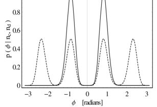
Figure 2: Probability density of the phase $p(\phi|m)$ for Fock state input (solid curve) and $N00N$ state input (dashed curve) for $N=25$ photons for measurement outcome $m=\{4_{c},21_{d}\}$.

Similarly, for a $N00N$-state input

$$|\Psi_{N00N}\rangle=\frac{1}{\sqrt{2}}\,\left[\;|N_{a},0_{b}\rangle+|0_{a},N_{b}\rangle\;\right]$$ (10)

the conditional probability is

$$P_{N00N}(n_{c},n_{d}|\phi)=\frac{1}{2\,}\frac{N\,!}{n_{c}!\;n_{d}!}\delta_{N,\,n_{c}\,+\,n_{d}}\,\left[\sin^{n_{c}}(\frac{\phi}{2})\cos^{n_{d}}(\frac{\phi}{2})+(-1)^{n_{c}}\sin^{n_{d}}(\frac{\phi}{2})\cos^{n_{c}}(\frac{\phi}{2})\right]^{2}.$$ (11)

It is clear that the probabilities $P_{N}(n_{c},n_{d}|\phi)$ and $P_{N00N}(n_{c},n_{d}|\phi)$, have multiple peaks, and therefore the resulting probability densities for the phase, $p(\phi|n_{c},n_{d})$ given by Eq.(4), also have multiple peaks. For a given $N$-photon Fock state input into port “a” and vacuum input into port “b”, the probability distribution $p(\phi|n_{c},n_{d})$ has either one or two peaks, depending on the measurement outcome. For the $N$-photon (entangled) $N00N$ state input, the probability distribution $p(\phi|n_{c},n_{d})$ has one, two, three, or four peaks, depending on the measurement outcome. See Figure 2 for an example plot of $p(\phi|n_{c},n_{d})$ for Fock state and $N00N$ state input for measurement outcome $\{4_{c},21_{d}\}$. There is more ambiguity in estimating the phase from the phase probability density for $N00N$ state input than Fock state input, because there are more peaks.

For input states with increasing photon number, the probability densities, $p(\phi|n_{c},n_{d})$, have narrower peaks, but the number of peaks remains the same: one or two for Fock state input, and one, two, three, or four peaks for $N00N$ state input.

When the interferometer is used as a sensor, it can be thought of as transmitting information about the phase to the experimenter via each measurement outcome. As described above, due to multiple peaks in the phase distribution, we do not attempt to use the width of the probability distributions to describe the quality of this sensor. Instead, we use the Shannon mutual information, given in Eq.(5), as a measure of the fidelity of an interferometric sensor. For the case of Fock state and $N00N$ state input, the mutual information, $H(\Phi\colon\!M)$, is plotted in Figure 3. In both cases, the fidelity of the interferometer, acting like a sensor, increases with increasing photon number due to the increased information carrying capacity of a higher-dimensional output alphabet associated with the $N+1$ measurement outcomes $\{n_{c},n_{d}\}$. However, for the same photon number input, the fidelity of the interferometer is clearly greater for Fock state input than for $N00N$ state input. This shows how the mutual information is sensitive to the number of peaks and not just the width $\Delta\phi$ of a single peak. Clearly, Fock states can carry more information about the phase to the measurement outcomes than $N00N$ states. This striking result demonstrates that the use of entangled input states does not lead to improvement over Fock state inputKapale2005 .

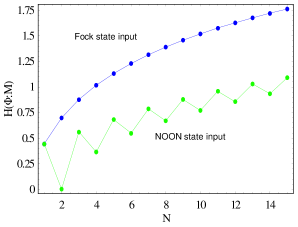
Figure 3: The mutual information $H(\Phi\colon\!M)$ is plotted vs. photon number for the case of N-photon Fock state input into port “a” (blue dots) and for an N-photon $N00N$ state input (green dots). Lines connect successive photon number points.

In order to optimize the Mach-Zehnder sensor, we can consider a more general class of states $|\Psi_{in}\rangle=\sum\limits_{n=0}^{N}\,c_{n}\,|\,n_{a,}\,(N-n)_{b}\,\rangle$, where $c_{n}$ are complex coefficients. The sensor can be optimized by finding the $N+1$ coefficients that maximize the fidelity, $H(\Phi\colon\!M)$, subject to the normalization constraint $\langle\Psi_{in}|\Psi_{in}\rangle=1$.

Work is in progress to analyze the mutual information for repeating the experiment $N$ times for arbitrary input states. An interesting example is the case when one-photon is input into port “a” and vacuum is input into port “b”. When the experiment is repeated $N$ times, with $M_{0\text{ }}$ outcomes $\{0_{c},1_{d}\}$ and $M_{1\text{ }}$ outcomes $\{1_{c},0_{d}\}$, where $N=$ $M_{0\text{ }}+M_{1\text{ }}$, the mutual information $H(\Phi\colon\!M)$ vs. $N$ is identical to that of Fock state input with the same $N$.

Summary. We have considered a generic Mach-Zehnder optical interferometer operating as a sensor of a classical field. Using a Bayesian analysis, we have shown that the conditional probability distribution for the phase shift, $p(\phi|n_{c},n_{d})$, has multiple peaks and is not adequately described by the standard deviation $\Delta\phi$, which has been used in discussion of the the standard limit ($\Delta\phi_{SL}\sim 1/\sqrt{N}$) and the Heisenberg limit ($\Delta\phi_{HL}\sim 1/N$) .

We proposed an alternative metric–called the fidelity of the interferometer–which is the Shannon mutual information, $H(\Phi\colon\!M)$, between the phase shift $\phi$ and the possible measurement outcomes $m$. For an interferometer used as a quantum sensor, we have shown that the fidelity is a measure of the quality of a sensor to detect external classical fields.

For the case of a generic Mach-Zehnder optical interferometer, we found the surprising result that entangled $N00N$ state input leads to a lower fidelity than Fock state input, for the same photon number. This result is intuitively understood because there are a larger number of peaks (bigger ambiguity in phase) in $p(\phi|n_{c},n_{d})$ for $N00N$ state input than for Fock state input.

The interferometer fidelity that we proposed is applicable to a wide variety of optical and matter wave interferometers, with arbitrary number of input/output ports. This measure of interferometer fidelity can be used as a metric for quantum interferometric sensors of classical fields, such as gravitational wave sensors, as well as optical gyroscopes and matter-wave gyroscopes based on BEC.

- (1) R. M. Godun, M. B. d’Arcy, G. S. Summy and K. Burnett, Contemporary Physics, 42, 77 (2001).
- (2) V. Giovannetti, S. Lloyd, and L. Maccone, Phys. Rev. Lett. 96, 010401 (2006).
- (3) K. Thorne, Rev. Mod. Phys. 52, 285 (1980).
- (4) W. W. Chow, J. Gea-Banacloche, L. M. Pedrotti, V. E. Sanders, W. Schleich, M. O. Scully, Rev. Mod. Phys. 57, 61 (1985).
- (5) G. Bertocchi, O. Alibart, D. B. Ostrowsky, S. Tanzilli and P. Baldi, J. Phys. B 39, 1011 (2006).
- (6) F. Zimmer and M. Fleischhauer, Phys. Rev. Lett. 92, 253201 (2004).
- (7) S. Gupta, K. W. Murch, K. L. Moore, T. P. Purdy, and D. M. Stamper-Kurn, Phys. Rev. Lett. 95, 143201 (2005)
- (8) Y.-J. Wang, D. Z. Anderson, V. M. Bright, E. A. Cornell, Q. Diot, T. Kishimoto, M. Prentiss, R. A. Saravanan, S. R. Segal, and S. Wu, Phys. Rev. Lett. 94, 090405 (2005).
- (9) O. I. Tolstikhin, T. Morishita, and S. Watanabe, Phys. Rev. A 72, 051603(R) (2005).
- (10) L. D. Didomenico, H. Lee, P. Kok, and J. P. Dowling, in Quantum Sensing and Nanophotonic Devices, edited by M. Razeghi, G. J. Brown, Proc. of SPIE Vol. 5359 (SPIE, Bellingham, WA, 2004).
- (11) K. T. Kapale, L. D. Didomenico, H. Lee, P. Kok, J. P. Dowling, quant-ph/0507150.
- (12) C. M. Caves, Phys. Rev. D 23, 1693 (1981).
- (13) R. S. Bondurant and J. H. Shapiro, Phys. Rev. D 30, 2548 (1984).
- (14) B. Yurke, Phys. Rev. Lett. 56, 1515 (1986).
- (15) B. Yurke, S. L. McCall, and J. R. Klauder, Phys. Rev. A 33, 4033 (1986).
- (16) H. P. Yuen, Phys. Rev. Lett. 56, 2176 (1986).
- (17) M. J. Holland and K. Burnett, Phys. Rev. Lett. 71, 1355 (1993).
- (18) J. P. Dowling, Phys. Rev. A 57, 4736 (1998).
- (19) T. Kim, O. Pfister, M. J. Holland, J. Noh, and J. L. Hall,Phys. Rev. A 57, 4004 (1998).
- (20) R. C. Pooser and O. Pfister, Phys. Rev. A 69, 043616 (2004).
- (21) L. Pezzé and A. Smerzi, quant-ph/0511059; quant-ph/0508158 v2;
- (22) L. Pezzé and A. Smerzi, Phys. Rev. A, 73, 011801 R (2006).
- (23) W. Heisenberg, Z. Phys. 43, 172 (1927).
- (24) C. W. Helstrom, Quantum Detection and Estimation Theory, Academic Press, New York (1976).
- (25) C. E. Shannon, The Bell System Technical Journal, 27, 379 (1948).
- (26) See also, M. A. Nielsen, I. L. Chuang, Quantum Computation and Quantum Information, Cambridge University Press, New York (2000).
- (27) M. W. Mitchell, J. S. Lundeen and A. M. Steinberg, Nature 429, 161 (2004).