Università degli Studi di Pavia

 

Facoltà di Scienze MM.FF.NN.

Dipartimento di Fisica “A. Volta”

Optimization and Realization
of Quantum Devices
PhD Thesis

by Francesco Buscemi

Supervisor: Chiar.mo Prof. Giacomo Mauro D’Ariano

Referee: Chiar.mo Prof. Francesco De Martini

XVIII ciclo, A. A. 2002/2005
  last version: February 29, 2024

Aspice convexo nutantem pondere mundum
terrasque tractusque maris caelumque profundum.

Behold the world swaying her convex mass,

lands and spaces of sea and depth of sky.

(Vergilius, Ecloga IV)

Preface Note

This manuscript must be intended as an informal review of the research works carried out during three years of PhD. “Informal” in the sense that technical proofs are often omitted (they can be found in the papers) as one could do for a presentation in a public talk. Clearly, some background of Quantum Mechanics is needed, even if I tried to minimize the prerequisites.

Contents

1. Preface Note
2. Introduction
3. 1 Quantum Measurements, Operations, and Physical Models
   1. 1.1 Classical and quantum events
   2. 1.2 Notations
   3. 1.3 Quantum measurements statistics: POVM’s
   4. 1.4 Quantum operations and instruments
      1. 1.4.1 State collapse postulate
      2. 1.4.2 Quantum operations
      3. 1.4.3 Instruments
   5. 1.5 Physical realizations
      1. 1.5.1 Levels of description of quantum measurements
      2. 1.5.2 Example: standard coupling
      3. 1.5.3 Example: embedding and optimal phase measurement
   6. 1.6 Repeatable measurements
4. 2 Characterization and Optimization of Quantum Devices
   1. 2.1 Choi-Jamiołkowski isomorphism
   2. 2.2 Group-theoretical techniques
      1. 2.2.1 Elements of group theory
      2. 2.2.2 Invariant operators and covariant channels
      3. 2.2.3 Example: $\mathbb{SU}(d)$-covariance
      4. 2.2.4 Example: $\mathbb{U}(1)$-covariance
      5. 2.2.5 Example: permutation group invariance
   3. 2.3 Optimization in a covariant setting
   4. 2.4 Universally covariant channels
      1. 2.4.1 Optimal universal cloning
      2. 2.4.2 Optimal universal NOT-gate
      3. 2.4.3 Universal qubit superbroadcasting
   5. 2.5 Phase-covariant channels
      1. 2.5.1 Optimal phase-covariant cloning
      2. 2.5.2 Optimal phase-covariant NOT-gate
      3. 2.5.3 Phase-covariant qubit superbroadcasting
5. 3 Realization of Quantum Devices
   1. 3.1 Unitary dilations of a channel
      1. 3.1.1 Stinespring dilation
      2. 3.1.2 Unitary dilation
   2. 3.2 Explicit realizations
      1. 3.2.1 Universal NOT and cloning gates
      2. 3.2.2 Phase-covariant cloning and economical maps
      3. 3.2.3 Phase-covariant NOT-gate
6. 4 The Role of Noise in Quantum Processes
   1. 4.1 Clean POVM’s
      1. 4.1.1 Postprocessing of output data
      2. 4.1.2 Preprocessing of input states
      3. 4.1.3 Positive maps
   2. 4.2 Inverting decoherence
      1. 4.2.1 Convex structure of decoherence maps
      2. 4.2.2 Correcting decoherence by measuring the environment
7. List of Publications
8. References

Introduction

To handle information is to handle physical systems, and viceversa. Hence, the ultimate limits in manipulating and distributing information are posed by the very laws of physics. This is true in the classical framework (e. g. Landauer’s principle) and in the quantum framework, where the rules of Quantum Mechanics give rise to new—and often not yet completely understood—restrictions and advantages to information processing and distribution. Quantum Information Theory is devoted to the investigation of the theoretical limits Quantum Mechanics establishes when dealing with information encoded on quantum systems. This thesis treats the problem of processing quantum information in an optimal way by means of physically realizable devices. In fact, linearity of Quantum Mechanics forbids basic processings of classical information—like e. g. copying-, broadcasting-, and NOT-gates—to properly work on an unknown quantum state. The first natural question is then: How well can we approximate such transformations and which are the physical devices that realize these approximations?

In contrast to its classical counterpart, quantum information is very sensitive to noise. In a realistic setup, it is unreasonable to completely rule out noise, since the least interaction with the sorroundings can cause the system to be irreversibly disturbed. This fact raises the need of designing methods to encode quantum information in a way that is robust with respect to noise. But in order to do this, we have to provide a model for the noise. In this sense, also noise can be viewed as a kind of processing of quantum states: a “nasty” processing, nonetheless obeying the same laws of Quantum Mechanics as “good” processings do. The second natural question is then: What is the role of noise in a realistic setup and how can we control it?

In order to answer both questions, we clearly need to work in full generality. The appropriate mathematical tool to do this is provided by the concept of quantum channel. It encloses all possible deterministic transformations of quantum states allowed by the postulates of Quantum Mechanics. In Chapter 1 we review the mathematical formalism describing quantum measurements and quantum state transformations. We face problems, such as quantum state preparation and repeatability of quantum measurements, which, even though they reach back to the beginnings of quantum theory, have been revived and put into a new light by the recent developments in the experimental techniques.

Chapter 2 is concerned with the analysis of quantum channels. Exploiting the convex structure of the set of channels, we explicitly single out those that constitute the best quantum versions of the intrisically classical copying-, broadcasting-, and NOT-gates. We introduce the general theory on which such optimization relies, and present group theoretical techniques to analyse the common situation in which symmetries of the set of input quantum states, after the action of the channel, propagate to the output. This is the framework of covariant channels. It is very useful to describe many physical situations and, at the same time, it permits an analytical approach.

Quantum channels are more general to describe changes of quantum states than unitary evolutions controlled by Schrödinger’s equation. Nonetheless, it is well known that every quantum channel is the transformation that a system undergoes when unitarily interacting with an auxiliary quantum system—the so-called ancilla—that is discarded after the interaction took place. Actually, this is the only way to deterministically realize a non-unitary quantum channel. In Chapter 3 we propose feasible implementations for some of the channels constructed in Chapter 2, providing the ancillary quantum state and the global unitary interaction. This is just a first step towards the experimental realization which remains a far more difficult task, however, the setup we propose to optimally copy quantum systems, in the case of qubits (i. e. two-levels systems) coincides with the one already used in experiments. This is encouraging in view of a possible generalization of experimental techniques to higher dimensional quantum systems.

The thesis ends with Chapter 4 which deals with classical and quantum noise. Noise is considered as acting both on the measuring apparata and on the quantum states. More specifically, we introduce a (partial) ordering on the convex set of measuring devices. It allows us to characterize “clean” devices, namely, those which are not affected by quantum and/or classical noise. Interestingly enough, we show that such ordering is able to single out von Neumann’s observables as “particularly nice” measuring apparata. This gives an operational characterization for the usually postulated concept of observable. We then focus attention on the specific model of noise called decoherence. Decoherence acts destroying quantum superpositions, thus making ineffective all quantum improvements on the classical approach. On the other side, decoherence possesses also foundational interest since it represents the favourite tool to explain the quantum-to-classical transition. The process called decoherence is actually a convex set of commuting channels satisfying very restrictive properties. Applying techniques described in Chapters 2 and 3, we provide a method to invert decoherence and restore quantum superpositions by a feedback control from the environment. This means that measuring a suitable observable of the environment’s degrees of freedom, and then performing on the system a suitable unitary transformation dependent on the measurement result, it is possible to completely cancel the effect of decoherence.

Chapter 1 Quantum Measurements, Operations, and Physical Models

1.1 Classical and quantum events

Given a finite probabilistic space $\Omega=\{1,\dots,N\}$, it is possible to define probability distributions $P=\{p_{1},\dots,p_{N}\}$ on $\Omega$, where $0\leq p_{i}\leq 1$, $\sum_{i}p_{i}=1$. The set of all probability distributions on $\Omega$, ${\sf P}(\Omega)$, is a convex set. It is simple to recognize its extremal points as the delta-distributions $p_{i}=\delta_{ij}$. Such a structure for ${\sf P}(\Omega)$ can be rephrased saying that ${\sf P}(\Omega)$ is a simplex, namely, a convex set whose elements are uniquely expressed as a convex combination of extremal points. Random variables on $\Omega$ are defined as mappings $X$ from $\Omega$ into a set of “values” $\Upsilon$. Such values can be numbers, tensors, or whatever objects. When $\Upsilon$ is a real vector space, it is well-defined the mean value of $X:\Omega\to\Upsilon$, given $P\in{\sf P}(\Omega)$, as $\bar{X}\equiv\sum_{i}p_{i}X(i)$. The set of random variables on $\Omega$ forms a commutative algebra (under point-wise multiplication). Events are particular random variables where $\Upsilon$ is the two-values set $\{0,1\}$. In the classical case, events form a boolean algebra: Given two events $E_{1},E_{2}:\Omega\to\{0,1\}$, once defined two binary operations $\land$ and $\lor$ as

$$E_{1}\land E_{2}\equiv E_{1}\cdot E_{2},\qquad E_{1}\lor E_{2}\equiv E_{1}+E_{2}-E_{1}\cdot E_{2},$$ (1.1)

where “$\cdot$” is the point-wise multiplication, it is straightforward to verify that all properties of a boolean algebra are satisfied.

Consider now a $N$-dimensional complex vector space $\mathscr{H}$. The analogue of probability distributions are $N\times N$ density matrices $\rho$, i. e. positive semi-definite trace-one matrices. The analogue of random variables are $N\times N$ hermitian matrices $X$. Since random variables, usually called observables, are hermitian, they admit a spectral decomposition $X=\sum_{j}x_{j}\Pi_{j}^{X}$, where $\Pi_{j}^{X}$ are orthogonal projections (of rank greater than one, in case of degeneracy). Density matrices, usually called states, define probability distributions over the spectrum of an observable, by means of the formula $\mu_{\rho}^{X}(x_{j})\equiv\operatorname{Tr}[\rho\Pi_{j}^{X}]$. The mean value of an observable $X$, given a state $\rho$, is well-defined as $\bar{X}\equiv\operatorname{Tr}[\rho X]$. The non-commutative analogue of events are projections $E_{i}=E_{i}^{2}$. The set of quantum events ${\sf E}(\mathscr{H})$, called quantum logic, has two binary operations $\land$ and $\lor$ defined as

$$E_{1}\land E_{2}\equiv E_{1}E_{2},\qquad E_{1}\lor E_{2}\equiv E_{1}+E_{2}-E_{1}E_{2},$$ (1.2)

where now the multiplication is the usual (non-commutative) matrix multiplication.

The fundamental differences between the classical model and the quantum model are the following (and they are basically equivalent):

1. the quantum logic is not a boolean algebra, since the distributivity law does not hold (beacause of the non-commutativity of the matrix product);

2. the convex set of states on $\mathscr{H}$ is not a simplex, but it is strongly convex, whence quantum states admit many equivalent ensemble decompositions;

3. the algebra of observables on $\mathscr{H}$ is non-commutative.

See also the introduction paragraphs in [1] and [2].

1.2 Notations

To each quantum system, it is associated a complex separable Hilbert space $\mathscr{H}$, equipped with the inner product $\langle\psi|\phi\rangle$, linear in $\phi$ and antilinear in $\psi$, following Dirac notation. The set of bounded operators on $\mathscr{H}$ will be denoted as ${\sf B}(\mathscr{H})$. An operator $X$ is called self-adjoint if it is densely defined and $X=X^{\dagger}$ on its domain. Self-adjoint operators are called observables and are in correspondence with orthogonal resolutions of the identity by means of the formula

$$X=\int_{-\infty}^{+\infty}x\textrm{d}\Pi^{X}(x),\qquad I=\int_{-\infty}^{+\infty}\textrm{d}\Pi^{X}(x).$$ (1.3)

Positive semi-definite trace-one operator $\rho\in{\sf T}^{+}(\mathscr{H})$ are called state. We will denote the set of states of a system $\mathscr{H}$ as ${\sf S}(\mathscr{H})$. Since they are all compact operators, states can be essentially viewed as infinite density matrices, also in the infinite dimensional case, with no relevant differences from the usual finite dimensional setting. From now on, if not otherwise specified, we will deal with finite $d$-dimensional Hilbert spaces isomorphic to $\mathbb{C}^{d}$, for which all linear operators are everywhere defined, bounded and trace-class, and the self-adjointness coincides with hermiticity. Moreover, spectral resolutions are all discrete, i. e. $X=\sum_{j}x_{j}\Pi_{j}^{X}$.

Composite systems carry a tensor-product Hilbert space, $\mathscr{H}_{1}\otimes\mathscr{H}_{2}\otimes\cdots\otimes\mathscr{H}_{N}$. Bounded operators ${\sf B}(\mathscr{H})$ form themselves a Hilbert space isomorphic to
$\mathscr{H}\otimes\mathscr{H}\equiv\mathscr{H}^{\otimes 2}$. Once fixed a basis $\mathbf{b}=\{|i\rangle\}$ for $\mathscr{H}$, we define the following isomorphism between operators in ${\sf B}(\mathscr{H})$ and vectors in $\mathscr{H}^{\otimes 2}$:

$$X=\sum_{ij}X_{ij}|i\rangle\langle j|\longleftrightarrow|X\rangle\!\rangle\equiv\sum_{ij}X_{ij}|i\rangle\otimes|j\rangle,$$ (1.4)

satisfying

1. $\langle\!\langle X|Y\rangle\!\rangle=\operatorname{Tr}[X^{\dagger}Y]$, i. e. the Hilbert-Schmidt product;

2. $(X\otimes Y)|Z\rangle\!\rangle=|XZY^{T}\rangle\!\rangle$, where $Y^{T}$ denotes the transposition with respect to the fixed basis $\mathbf{b}$;

3. $\operatorname{Tr}_{1}[|X\rangle\!\rangle\langle\!\langle Y|]=X^{T}Y^{*}$, where $Y^{*}$ denotes the complex conjugation with respect to $\mathbf{b}$;

4. $\operatorname{Tr}_{2}[|X\rangle\!\rangle\langle\!\langle Y|]=XY^{\dagger}$.

With this notation the state $|I/\sqrt{d}\rangle\!\rangle$ is the maximally entangled state on $\mathscr{H}^{\otimes 2}$:

$$\frac{1}{\sqrt{d}}|I\rangle\!\rangle=\frac{1}{\sqrt{d}}\sum_{i}|i\rangle\otimes|i\rangle.$$ (1.5)

Such a state will play a major role in the characterization of quantum devices.

1.3 Quantum measurements statistics: POVM’s

Given a state $\rho$ and an observable $X=\sum_{j}x_{j}\Pi_{j}^{X}$, the statistical postulate states that: The probability of obtaining a result $x_{j}$ within a set $\Delta=\{x_{j}\}_{j\in J}$ is given by

$$p(x_{j}\in\Delta)=\operatorname{Tr}\left[\rho\sum_{j\in J}\Pi_{j}^{X}\right].$$ (1.6)

This means, as we already saw, that a state induces a probability measure $\mu_{\rho}^{X}(x_{j})=\operatorname{Tr}[\rho\Pi_{j}^{X}]$ over the set of outcomes for a given observable.

It is clear that, apart from the actual measured value $x_{j}$ of the observable $X$, the statistics of the outcomes is completely determined by the structure of its spectral resolution $\{\Pi_{j}^{X}\}$. In the case of an observable, such $\Pi_{j}$’s are orthogonal projections, i. e. $\Pi_{i}^{X}\Pi_{j}^{X}=\Pi_{i}^{X}\delta_{ij}$, summing up to the identity, $\sum_{j}\Pi_{j}^{X}=I$. With a little abuse of terminology, from now on we will refer to an observable just as a set of orthogonal projections resolving the identity, and to the observable outcomes as the indices $j$’s labelling different $x_{j}$’s.

The concept of observable is generalized by the concept of positive operator-valued measure (POVM, for short), which is a set of positive operators $\mathbf{P}=\{P_{1},P_{2},\dots,P_{N}\}$ summing up to the identity $\sum_{i}P_{i}=I$. Notice that $P_{i}$’s need not to be orthogonal, not even projections, and the number of oucomes of $\mathbf{P}$, i. e. its cardinality $|{\mathbf{P}}|\equiv N$, can be larger than the Hilbert space dimension $d$. As before, also in the case of POVM’s, the probability of obtaining the $j$-th outcome, given the system in the state $\rho$, is postulated to be $\mu_{\rho}^{\mathbf{P}}(j)\equiv\operatorname{Tr}[\rho P_{j}]$.

We call a two-outcomes POVM $\mathbf{P}=\{P,I-P\}$ an effect or, equivalently, a property. According to [3] we say that an effect $\mathbf{P}=\{P,I-P\}$ describes a real property for the system $\mathscr{H}$ in the state $\rho$, if $\operatorname{Tr}[\rho P]=1$.

Finally, we introduce here the definition of range of a POVM, a concept we will extensively use in Chapter 4.

Definition 1.3.1 (POVM range)

Given a POVM $\mathbf{P}=\{P_{1},P_{2},\dots,P_{N}\}$, its range, denoted as ${\sf Rng}(\mathbf{P})$, is defined to be the convex set of probability distributions $\mathbf{p}=\{p_{1},p_{2},\dots,p_{N}\}$ obtained as $p_{i}=\operatorname{Tr}[\rho P_{i}]$, varying $\rho$ in all ${\sf S}(\mathscr{H})$.

Remark 1.3.2

Notice that, since $\rho$ in Definition 1.3.1 moves around the whole quantum states’ set, the range of a POVM identifies uniquely the POVM. In other words, the correspondence

$$\mathbf{P}\longleftrightarrow{\sf Rng}(\mathbf{P})$$ (1.7)

is one-to-one.

1.4 Quantum operations and instruments

Since now, we dealt only with the outcomes statistics. However, in order to completely describe the measurement statistics we need also to specify the state reduction from prior state $\rho$ to posterior state $\rho_{j}$ conditioned by the outcome $j$. The state reduction is nothing but a rule telling us which is the system’s state after the measurement has been performed and the outcome collected.

1.4.1 State collapse postulate

Von Neumann [4] derived the well-known state collapse rule starting from the following hypothesis:

1. the observable to be measured has discrete spectrum and it is non degenerate, namely all its eigenspaces are one-dimensional, in formula $X=\sum_{i}x_{i}|x_{i}\rangle\langle x_{i}|$;

2. the measurement is perfectly repeatable: Literally from von Neumann’s book “if a physical quantity is measured twice in succession in a system, then we get the same value each time”.

If such hypotheses are verified, then the system state after the measurement is

$$\rho\longmapsto\rho_{j}\equiv|x_{j}\rangle\langle x_{j}|.$$ (1.8)

Lüders [5] generalized von Neumann’s theorem to degenerate observables, introducing the postulate of minimum disturbance in the sense that a state, for which a property $\mathbf{P}$ is real, is left unchanged by a measurement of $\mathbf{P}$. According to Lüders’ rule, when measuring the observable $X=\sum_{i}x_{i}\Pi_{i}^{X}$ the system’s state after the measurement is

$$\rho\longmapsto\rho_{j}\equiv\frac{\Pi_{j}^{X}\rho\Pi_{j}^{X}}{\operatorname{Tr}[\rho\Pi_{j}^{X}]}.$$ (1.9)

The interpretation problems to which the state collapse postulate led are beyond the aim of this manuscript.

1.4.2 Quantum operations

The appropriate mathematical objects describing a general quantum state change are the so-called quantum operations [6]. A quantum operation ${\mathcal{E}}$, is a completely positive trace-non-increasing linear mapping from ${\sf T}^{+}(\mathscr{H})$ of an input system $\mathscr{H}$ to ${\sf T}^{+}(\mathscr{K})$ of an output system $\mathscr{K}$. The map ${\mathcal{E}}:{\sf T}^{+}(\mathscr{H})\to{\sf T}^{+}(\mathscr{K})$ is generally probabilistic, and the trace $\operatorname{Tr}[{\mathcal{E}}(\rho)]\leq 1$ represents the probability that the transformation

$$\rho\longmapsto\rho^{\prime}\equiv\frac{{\mathcal{E}}(\rho)}{\operatorname{Tr}[{\mathcal{E}}(\rho)]}$$ (1.10)

occurs. Deterministic quantum operations, i. e. completely positive trace-preserving maps such that $\operatorname{Tr}[{\mathcal{E}}(\rho)]=1$ for all $\rho\in{\sf S}(\mathscr{H})$, are called channels. All quantum operations admit the highly non-unique Kraus representation

$${\mathcal{E}}(\rho)=\sum_{j}E_{j}\rho E_{j}^{\dagger},$$ (1.11)

where $E_{j}$’s are linear operators from $\mathscr{H}$ to $\mathscr{K}$. Nonetheless, it is always possible to choose a Kraus representation such that $\operatorname{Tr}[E_{i}^{\dagger}E_{j}]=\|E_{i}\|^{2}_{2}\delta_{ij}$; we call it canonical Kraus representation. A quantum operation is a channel if and only if its Kraus operators satisfy the normalization condition

$$\sum_{i}E_{i}^{\dagger}E_{i}=I.$$ (1.12)

Remark 1.4.1

The Lüders’ recipe for state change clearly corresponds to a quantum operation ${\mathcal{E}}_{j}(\rho)=\Pi_{j}^{X}\rho\Pi_{j}^{X}$. Notice that the average reduced state $\bar{\rho}\equiv\sum_{i}p(i)\rho_{i}$ can be read as the output of the channel ${\mathcal{E}}(\rho)=\sum_{i}\Pi_{i}^{X}\rho\Pi_{i}^{X}$.

Every quantum operation ${\mathcal{E}}:{\sf S}(\mathscr{H})\to{\sf S}(\mathscr{K})$ induces naturally a quantum operation ${{\mathcal{E}}}^{\tau}$ from ${\sf B}(\mathscr{K})$ to ${\sf B}(\mathscr{H})$ by means of the duality relation $\operatorname{Tr}[{\mathcal{E}}(\rho)X]=\operatorname{Tr}[\rho{{\mathcal{E}}}^{\tau}(X)]$, valid for all $\rho\in{\sf S}(\mathscr{H})$ and $X\in{\sf B}(\mathscr{K})$. The map ${{\mathcal{E}}}^{\tau}$ is called the dual map, and ${{\mathcal{E}}}^{\tau}(I_{\mathscr{K}})=I_{\mathscr{H}}$ if and only if ${\mathcal{E}}$ is a channel.

Remark 1.4.2

Given a measurement whose outcomes statistics is described by means of the POVM $\mathbf{P}$, there exist many different channels associated with $\mathbf{P}$. These channels are written as ${\mathcal{E}}^{\mathbf{P}}(\rho)=\sum_{i}{\mathcal{E}}_{i}^{\mathbf{P}}(\rho)$, with ${({\mathcal{E}}_{j}^{\mathbf{P}})}^{\tau}(I)=P_{j}$, and choosing between them correspond to assign a particular state reduction rule.

1.4.3 Instruments

In the modern formulation of Quantum Mechanics, the most general tool used to describe statistical correlations between the outcomes of successive measurements is given by the notion of (completely positive) instrument, which has been introduced by Davies and Lewis [7]. An instrument is basically a mapping $\mathfrak{I}$ from the set $\Omega$ of outcomes to the set of quantum operations on ${\sf S}(\mathscr{H})$, such that $\mathfrak{I}(\bigcup_{j\in J}j)=\sum_{j\in J}\mathfrak{I}(j)$ and $\mathfrak{I}(\Omega)$ is a channel. The fundamental result about instruments is the following [8]

Theorem 1.4.3 (Ozawa, 1984)

Every statistical measurement theory, consisting both of outcomes statistics and state reduction rule, can be described by means of an appropriate instrument.

Actually, instruments formalism has been introduced in literature mainly to handle the case of continuous outcome space $\Omega$, which is described as a standard Borel space equipped with a $\sigma$-algebra ${\mathfrak{B}}(\Omega)$. When $\Omega$ is discrete and subset of $\mathbb{R}$—as in our case—technical results become much simpler. For further details on the general case see [9].

Finally, we define a perfect instrument as an instrument such that $\mathfrak{I}(j)$ is a pure contractive map, i. e. $\mathfrak{I}(j)(\rho)=M_{j}\rho M_{j}^{\dagger}$, for all $j$. For example, Lüders instrument in Remark 1.4.1 is a perfect instrument with $M_{j}=\Pi_{j}^{X}$. The instrument in Remark 1.4.2 is perfect only if ${\mathcal{E}}_{j}^{\mathbf{P}}(\rho)=\sqrt{P_{j}}\rho\sqrt{P_{j}}$.

1.5 Physical realizations

Intruments provide both outcomes statistics and state reduction due to a measurement process. Implicitly, we assume that such a measurement is nondestructive, in the sense that the system is left in a state conditioned by the outcome and not, for example, absorbed by a counter or a calorimeter. The only reasonable way to look for an implementation of a nondestructive measuring process on a quantum system $\mathscr{H}$ is to engineer an indirect measurement scheme. This means that we make the system interact with an apparatus $\mathscr{A}$ and, after some time, we measure an observable $Y$ on the apparatus. In formula:

$$\mathfrak{I}(j)(\rho)=\operatorname{Tr}_{\mathscr{A}}\left[\left(I_{\mathscr{H}}\otimes\Pi_{j}^{Y}\right)U(\rho\otimes|a\rangle\langle a|)U^{\dagger}\right],$$ (1.13)

where $\{\Pi_{j}^{Y}\}_{j}$ is an orthogonal resolution of $I_{\mathscr{A}}$ coming from the diagonalization of $Y\in{\sf B}(\mathscr{A})$. Clearly such a procedure gives rise to an instrument, as described in the previous Section. Ozawa [8] proved the converse:

Theorem 1.5.1 (Ozawa, Indirect Measurement, 1984)

Every instrument $\mathfrak{I}$ admits an indirect measurement scheme as in Eq. (1.13).

The correspondence is not one-to-one: there are many different—though statistically equivalent—indirect measurement schemes producing the same instrument; conversely, given the indirect measurement scheme, the resulting instrument is unique.

1.5.1 Levels of description of quantum measurements

There are basically three ways to describe the statistical aspects of quantum measurements, depending on the level of details required:

1. One is interested only in the outcome statistics. Then the maximum generality lies in the concept of POVM, as we saw in Section 1.3. Notice that, given the outcome statistics for all quantum states, the POVM is defined uniquely—see Remark 1.3.2.

2. Also the state reduction rule is requested. The notion of instrument encloses all possible cases, see Section 1.4. Evidently, many different instruments produce the same outcome statistics, i. e. they all correspond to the same POVM.

3. The most detailed description characterizes even the state of the apparatus, the physical interaction between the system and the apparatus, and the observable to be measured on the apparatus. Clearly the same instrument is obtainable by means of different indirect measurement schemes.

Summarizing, given the outcome statistics, the POVM is uniquely defined. Given the POVM, there are many instruments describing it. Similarly, there are many indirect measurement schemes realizing a given instrument. The choice between different equivalent physical realizations of a measurement process can be made according only to “practical” considerations.

1.5.2 Example: standard coupling

Consider a discrete observable $X=\sum_{i}x_{i}\Pi_{i}^{X}$ of the system $\mathscr{H}$ in initial state $|\psi\rangle$ and let the apparatus system be $\mathscr{A}=L^{2}(\mathbb{R})$ in initial state $|\phi_{a}\rangle$. Now, let $\mathscr{H}$ and $\mathscr{A}$ interact in such a way that the the observable $X$ couples with the apparatus’ momentum $P_{a}$. This means that the unitary operator is

$$U=e^{-i\lambda X\otimes P_{a}}.$$ (1.14)

The momentum operator $P_{a}$ is the generator of translations, in the sense that

$$e^{-\frac{i}{\hslash}x_{0}P_{a}}\phi_{a}(x)=\phi_{a}(x-x_{0}),$$ (1.15)

where $\phi_{a}(x)=\langle x|\phi_{a}\rangle$. Hence, the initial system+apparatus state $|\psi\rangle\otimes|\phi_{a}\rangle$ evolves as

$$U|\psi\rangle\otimes\phi_{a}(x)=\sum_{i}\Pi^{X}_{i}|\psi\rangle\otimes\phi_{a}(x-\hslash\lambda x_{i}),$$ (1.16)

and, by making assumptions on the value of the coupling constant $\lambda$ and the initial state $|\phi_{a}\rangle$, it is always possible to obtain functions $\phi_{a}(x-\hslash\lambda x_{i})$ with (almost) disjoint supports. In other words, it is always possible to model an interaction between system and apparatus such that the indirect measurement is a position measurement on the apparatus—the usual “pointer position” measurement.

1.5.3 Example: embedding and optimal phase measurement

From the geometrical point of view, the unitary interaction of the system with a fixed ancilla state in the indirect measurement scheme (1.13) simply corresponds to a linear (isometrical) embedding of the system $\mathscr{H}$ into a composite Hilbert space $\mathscr{H}\otimes\mathscr{A}$. The measurement on the apparatus then defines a conditional expectation from $\mathscr{H}\otimes\mathscr{A}$ to $\mathscr{H}$, giving rise to probability and state reduction. An embedding into a larger space can always be described by means of an isometry $V$, i. e. a bounded operator such that $V^{\dagger}V=I$. If the input system state is $\rho$, then the embedded state—that is, the system+apparatus state after the interaction—is $U(\rho\otimes|a\rangle\langle a|)U^{\dagger}\equiv V\rho V^{\dagger}$.

In Ref. [10], we exploited an embedding for single-mode states of the electromagnetic field in order to achieve a physical realization of the optimal phase measurement. It is well known that the phase of the electromagnetic field does not correspond to any self-adjoint operator. Quantum estimation theory [1, 11] provides the optimal POVM for the phase measurement in terms of Susskind-Glogower operators

$$\textrm{d}\hat{\mu}(\phi)=\frac{\textrm{d}\phi}{2\pi}|e^{i\phi}\rangle\langle e^{i\phi}|,\quad\int_{0}^{2\pi}\textrm{d}\hat{\mu}(\phi)=I,$$ (1.17)

where $|e^{i\phi}\rangle\equiv\sum_{n=0}^{\infty}e^{i\phi\hat{n}}|n\rangle$. The optimal phase measurement outcomes distribution is then

$$\textrm{d}\mu_{\rho}^{\phi}=\frac{\textrm{d}\phi}{2\pi}\langle e^{i\phi}|\rho|e^{i\phi}\rangle.$$ (1.18)

Using the double-ket notation introduced in Section 1.2, consider now the eigenstates of the hetherodyne photocurrent $Z=a-b^{\dagger}$

$$\hat{Z}|D(z)\rangle\!\rangle=z|D(z)\rangle\!\rangle,$$ (1.19)

where $D(z)=e^{za^{\dagger}-z^{*}a}$ are the displacement operators, satisfying the completness relation

$$\int_{\mathbb{C}}\frac{\textrm{d}^{2}z}{\pi}|D(z)\rangle\!\rangle\langle\!\langle D(z)|=I^{\otimes 2}.$$ (1.20)

The following isometry

$$V=\frac{1}{\sqrt{2\pi}}\int_{\mathbb{C}}\textrm{d}^{2}\alpha f(|\alpha|)|D(\alpha)\rangle\!\rangle\langle e^{i\arg\alpha}|,\quad\int_{0}^{\infty}\textrm{d}t|f(t)|^{2}=\frac{1}{\pi}$$ (1.21)

embeds a single-mode state into a two-modes state in such a way that, measuring the hetherodyne photocurrent

$$\begin{split}p(z)&=\frac{1}{\pi}\operatorname{Tr}\left[V\rho V^{\dagger}\ |D(z)\rangle\!\rangle\langle\!\langle D(z)|\right]\\ &=\frac{1}{2}\left|f(|z|)\right|^{2}\langle e^{i\arg z}|\rho|e^{i\arg z}\rangle,\end{split}$$ (1.22)

one obtains the optimal phase distribution $\textrm{d}\mu_{\rho}^{\phi}$ as the marginal of $p(z)$ on the variable $\phi=\arg z$. Notice that here we are performing a joint measurement on both modes, not just an indirect measurement on the second mode. However, the form of the embedding $V$ provides a natural way to implement the phase POVM (1.17).

1.6 Repeatable measurements

In Subsection 1.4.1 we introduced the von Neumann-Lüders state collapse principle, derived from the hypothesis of discreteness of spectrum, repeatability, and minimum disturbance. In what follows, we derive all the consequences that arise from the only hypothesis of repeatability, thus obtaining the most general form of a repeatable measurement. See [12] for a detailed derivation.

First of all, why should we focus on repeatable measurements? Clearly, there are a lot of natural measurement schemes which are far from being repeatable, think of e. g. a photon counter or a fluorescent screen at the end of a Stern-Gerlach apparatus. In the past decades, however, technology of quantum experiments improved in such a way that nondestructive measurements on individual atomic objects are quite a common task, see e. g. one atom micro-masers and ions traps.

In the modern formulation of Quantum Mechanics, repeatability hypothesis has lost the in-principle relevance it enjoyed in the early foundational books as von Neumann’s. Nowadays, repeatability is understood just as a property which characterizes some particular measurement processes. More precisely, repeatable measurements are related to preparation procedures. In fact, preparing a quantum system in a particular state means preparing it in a state having some pre-specified real property, as defined in Section 1.3. For example, in order to prepare the pure state $|\psi\rangle$, one may take a collection of quantum systems and perform over them a repeatable measurement of the effect described by the POVM $\{|\psi\rangle\langle\psi|,I-|\psi\rangle\langle\psi|\}$. Of course, the preparation succeeds when the outcome $|\psi\rangle\langle\psi|$ comes out. Then, the von Neumann-Lüders state collapse rule tells us that the state of the system after measurement is in fact the pure state $|\psi\rangle$. In this sense, repeatable measurements have often been regarded as measurements of observables—projective orthogonal resolution of the identity—causing a collapse of the state on one of their eigenvectors.

In [12] we showed that there exist repeatable measurements which give rise to nonorthogonal POVM’s and, moreover, which do not even admit any eigenvector, that is to say, the reduced state is different at every repetition of the measurement. This result makes a clear separation between the concepts of repeatability, preparation and reality in Quantum Measurement Theory.

The starting point is the hypothesis of repeatability. A first consequence of this is due to Ozawa [8]:

Theorem 1.6.1 (Ozawa, Repeatable Measurements, 1984)

An instrument satisfies repeatability hypothesis only if it has discrete spectrum.

Then, perfect repeatable instruments are described by a set of contractions $\{M_{j}\}$ such that $\sum_{i}M_{i}^{\dagger}M_{i}=I$ and

$$\frac{\|M_{j}M_{k}|\psi\rangle\|}{\|M_{k}|\psi\rangle\|}=p(j|k)=\delta_{jk},$$ (1.23)

for all $j,k$ and all $|\psi\rangle\in\mathscr{H}$. The only technical point recalled in the paper is that, allowing for infinite dimensional Hilbert spaces, one has also to deal with properties of operators such as closeness. In our case, all $M_{i}$’s are bounded and everywhere defined, hence closed [13]. A close operator possesses closed range and kernel (the support is always closed since by definition it is the orthogonal complement of the kernel) and the Hilbert space $\mathscr{H}$ can hence be decomposed as

$$\mathscr{H}\simeq{\sf Ker}(M_{j})\oplus{\sf Supp}(M_{j})\simeq{\sf Rng}(M_{j})\oplus{\sf Rng}(M_{j})^{\perp},\qquad\forall j.$$ (1.24)

The consequences are the following:

1. All ranges, for different outcomes, must be orthogonal, i. e.

   $${\sf Rng}(M_{i})\perp{\sf Rng}(M_{j}),\quad i\neq j.$$ (1.25)

2. All ranges must be contained in respective supports, i. e.

   $${\sf Rng}(M_{i})\subseteq{\sf Supp}(M_{i}),\quad\forall i.$$ (1.26)

3. All $M_{i}$’s satisfy the condition

   $$M_{i}^{\dagger}M_{i}|_{{\sf Rng}(M_{i})}\equiv I_{{\sf Rng}(M_{i})}.$$ (1.27)

Now, the fundamental difference between operators on finite and infinite Hilbert spaces is that, in finite dimension, ${\sf Supp}(X)\simeq{\sf Rng}(X)$ always, while, in the infinite dimensional case, one can have ${\sf Supp}(X)\subset{\sf Rng}(X)$ or, viceversa, ${\sf Rng}(X)\subset{\sf Supp}(X)$, strictly. This holds basically because in the infinite dimensional case there exist proper subspaces with the same dimension as the whole Hilbert space $\mathscr{H}$. This observation lead us to the following:

Theorem 1.6.2

For finite dimensional systems, only observables admit repeatable measurement schemes, and the system state collapses according to the von Neumann-Lüders rule (1.9).

So the finite dimensional case describes precisely what one usually expects about the structure of repeatable measurements. It is nonetheless possible to construct a simple example in infinite dimension, enclosing all counter-intuitive features of the infinite dimensional case. Let us consider a two-outcomes POVM:

$$\begin{split}&P_{0}=p|0\rangle\langle 0|+\sum_{j=0}^{\infty}|2j+1\rangle\langle 2j+1|,\\ &P_{1}=(1-p)|0\rangle\langle 0|+\sum_{j=0}^{\infty}|2j+2\rangle\langle 2j+2|.\end{split}$$ (1.28)

Notice that $\mathbf{P}=\{P_{0},P_{1}\}$ is a nonorthogonal measurement. We can describe such a POVM by means of the following instrument:

$$\begin{split}&M_{0}=\sqrt{p}|1\rangle\langle 0|+\sum_{j=0}^{\infty}|2(j+1)+1\rangle\langle 2j+1|,\qquad M_{0}^{\dagger}M_{0}=P_{0},\\ &M_{1}=\sqrt{1-p}|2\rangle\langle 0|+\sum_{j=0}^{\infty}|2(j+1)+2\rangle\langle 2j+2|,\qquad M_{1}^{\dagger}M_{1}=P_{1},\end{split}$$ (1.29)

in the sense that, got the $i$-th outcome, the state changes as $M_{i}\rho M_{i}^{\dagger}$. Repeatability hypothesis can be simply checked. Analysing the structure of scheme (1.29) one recognizes a unilateral-shift behaviour of the kind $S|n\rangle=|n+1\rangle$. Actually, this unilateral-shift structure is a general feature of nonorthogonal repeatable measurements. Since $S$ does not admit any eigenvector, analogously the scheme (1.29) changes the system state at every repetition of the measurement and there are no states which are left untouched by such a scheme. In other words, in infinite dimensional systems there exist repeatable measurements which cannot satisfy minimum disturbance hypothesis, even in principle, and hence cannot be viewed as preparation procedures.

Chapter 2 Characterization and Optimization of Quantum Devices

In order to handle information encoded on quantum states we need to engineer astonishingly precise and accurate devices since the least loss of control in manipulating quantum systems can lead to extremely detrimental effects on the whole process. The theoretical investigation is the starting ground in designing such optimal quantum devices. This Chapter is devoted, first, to giving a complete and tractable characterization of quantum channels, second, to exploiting such characterization to single out optimal devices according to particular figures of merit that we will introduce and explain from time to time.

The basic assumption we will adopt is to consider input quantum states belonging to sets obeying some symmetry constraints—i. e. satisfying invariance properties under the action of some groups of transformations. Moreover, we will choose figures of merit conforming in a natural way to the same symmetry constraints. These two conditions lead to the very well established mathematical framework of covariant channels, for which the characterization simplifies, making explicit calculations analytically solvable. Actually, covariant channels form convex sets whose structure is (in some cases) known and optimal devices lie on the border of such sets. In this way, the problem resorts to a semi-definite linear program.

In particular, we will focus on channels optimally approximating the impossible tasks of copying, broadcasting, and performing NOT on unknown quantum states. The symmetries we will deal with are universal symmetry (invariance under the action of $\mathbb{SU}(d)$), phase-rotations symmetry (invariance under the action of $\mathbb{U}(1)^{\times d}$), and invariance under the group of permutations.

2.1 Choi-Jamiołkowski isomorphism

A useful tool to characterize quantum channels in finite dimensional systems is the Choi-Jamiołkowski [14, 15, 16] isomorphism—one-to-one correspondence—between channels ${\mathcal{E}}:{\sf S}(\mathscr{H})\to{\sf S}(\mathscr{K})$ and positive operators $R_{\mathcal{E}}$ on $\mathscr{K}\otimes\mathscr{H}$ defined as follows:

$$R_{\mathcal{E}}=({\mathcal{E}}\otimes{\mathcal{I}})|I\rangle\!\rangle\langle\!\langle I|\longleftrightarrow{\mathcal{E}}=\operatorname{Tr}_{\mathscr{H}}\left[\left(I\otimes\rho^{T}\right)R_{\mathcal{E}}\right],$$ (2.1)

where ${\mathcal{I}}$ is the identity map on ${\sf S}(\mathscr{H})$, $|I\rangle\!\rangle=\sum_{i}|i\rangle\otimes|i\rangle$ is the maximally entangled (non normalized) vector in $\mathscr{H}\otimes\mathscr{H}$, and $O^{T}$ denotes the transposition with respect to the fixed basis used to write $|I\rangle\!\rangle$. Different Kraus representations for ${\mathcal{E}}(\rho)=\sum_{i}E_{i}\rho E_{i}^{\dagger}$ correspond to different ensemble representations for $R_{\mathcal{E}}=\sum_{i}|E_{i}\rangle\!\rangle\langle\!\langle E_{i}|$, the canonical being the diagonalizing one. Trace-preservation constraint $\sum_{i}E_{i}^{\dagger}E_{i}=I_{\mathscr{H}}$ rewrites as $\operatorname{Tr}_{\mathscr{K}}\left[R_{\mathcal{E}}\right]=I_{\mathscr{H}}$.

Choi-Jamiołkowski isomorphism (2.1) turns out to be very useful in describing covariant channels. In the following Section we shall recall some basic notions about group theory.

2.2 Group-theoretical techniques

2.2.1 Elements of group theory

A unitary (projective) representation on $\mathscr{H}$ of the group $\mathbf{G}$ is a homomorphism $\mathbf{G}\ni g\mapsto U_{g}\in{\sf B}(\mathscr{H})$, with $U_{g}$ unitary operator, such that the composition law is preserved:

$$U_{g}U_{h}=\omega(g,h)U_{gh}.$$ (2.2)

The cocycle $\omega(g,h)$ is a phase, i. e. $|\omega(g,h)|=1$, for all $g,h\in\mathbf{G}$, and it satisfies the relations

$$\begin{split}&\omega(gh,k)\omega(g,h)=\omega(g,hk)\omega(h,k)\\ &\omega(g,g^{-1})=1.\end{split}$$ (2.3)

A unitary representation is called irreducible (UIR) if there are no proper subspaces of $\mathscr{H}$ left invariant by the action of all its elements. Two irreducible representations $U^{1}$ and $U^{2}$ of $\mathbf{G}$ on $\mathscr{H}_{1}$ and $\mathscr{H}_{2}$, respectively, are called equivalent if there exists a unitary $T:\mathscr{H}_{1}\to\mathscr{H}_{2}$ such that $TU^{1}_{g}=U^{2}_{g}T$, for all $g\in\mathbf{G}$. The fundamental result concerning UIR’s of a group is the following:

Lemma 2.2.1 (Schur)

Let $U^{1}$ and $U^{2}$ be two UIR of $\mathbf{G}$ on $\mathscr{H}_{1}$ and $\mathscr{H}_{2}$, respectively. Let $B:\mathscr{H}_{1}\to\mathscr{H}_{2}$ a (bounded) operator such that:

$$BU^{1}_{g}=U^{2}_{g}B,$$ (2.4)

for all $g\in\mathbf{G}$. Then:

1. $U^{1}$ and $U^{2}$ equivalent $\Longrightarrow$ $B\propto T$;

2. $U^{1}$ and $U^{2}$ inequivalent $\Longrightarrow$ $B=0$.

Remark 2.2.2 (Abelian groups)

From Schur Lemma simply follows that fact that, if the group $\mathbf{G}$ is abelian, nemely $g_{1}g_{2}=g_{2}g_{1}$ for all $g_{1},g_{2}\in\mathbf{G}$, then all its UIR’s are one-dimensional. In fact, all $U_{g}$’s must be proportional to the same unitary operator $T$ and they are all simultaneously diagonalizable, hence reducible on direct sums of one-dimensional invariant subspaces.

2.2.2 Invariant operators and covariant channels

Let $W_{g}$ a reducible unitary representation of $\mathbf{G}$ on $\mathscr{H}$. Then $\mathscr{H}$ can be decomposed into a direct sum of minimal invariant subspaces:

$$\mathscr{H}\simeq\bigoplus_{i}\mathscr{H}_{i}.$$ (2.5)

Each $\mathscr{H}_{i}$ supports one UIR of $\mathbf{G}$. Some UIR’s can be equivalent or inequivalent. Let us group equivalent UIR’s under an index $\mu$ labelling different equivalence classes, and let an additional index $i_{\mu}$ span UIR’s among the same $\mu$-th equivalence class. Since equivalent UIR are supported by isomorphic subspaces, i. e. $\mathscr{H}_{i_{\mu}}\simeq\mathscr{H}_{j_{\mu}}\simeq\mathscr{H}_{\mu}$ for all $i_{\mu},j_{\mu}$ in the same $\mu$-th class, we can rewrite the decomposition (2.5) as

$$\mathscr{H}\simeq\bigoplus_{\mu}\mathscr{H}_{\mu}\otimes\mathbb{C}^{d_{\mu}},$$ (2.6)

where $d_{\mu}$ is the cardinality (degeneracy) of the $\mu$-th equivalence class. Decomposition (2.6) is usually called Wedderburn’s decomposition [17], the spaces $\mathscr{H}_{\mu}$ are called representation spaces, and the spaces $\mathbb{C}^{d_{\mu}}$ multiplicity spaces. Then, the following decomposition for the representation $W_{g}$ holds

$$W_{g}=\bigoplus_{\mu}W_{g}^{\mu}\otimes I_{d_{\mu}}.$$ (2.7)

With Eq. (2.7) at hand, it is simple to derive the form of an operator $B$, invariant under the action of the reducible representation $W_{g}$, i. e.

$$W_{g}^{\dagger}BW_{g}=B,\qquad\forall g\in\mathbf{G}.$$ (2.8)

Since the above implies $[B,W_{g}]=0$, for all $g$, then:

$$B=\bigoplus_{\mu}I^{\mu}\otimes B_{d_{\mu}},$$ (2.9)

where $B_{d_{\mu}}$ is an operator on $\mathbb{C}^{d_{\mu}}$. In other words, the operator $B$ is in a block-form since it cannot connect inequivalent representations and can act non-trivially only on multiplicity spaces of the representation $W_{g}$. This is precisely what is contained in the Schur’s Lemma 2.2.1.

Now, consider a family of quantum states ${\sf F}\subseteq{\sf S}(\mathscr{H})$ that is invariant under the action of a group $\mathbf{G}$, namely $U_{g}\rho U_{g}^{\dagger}\in{\sf F}$ for all $g\in\mathbf{G}$ and all $\rho\in{\sf F}$. The group, and then the family ${\sf F}$, can be discrete as well as continuous. A channel ${\mathcal{E}}:{\sf F}\to{\sf S}(\mathscr{K})$ is said to be covariant under the action of the group $\mathbf{G}$ if

$${\mathcal{E}}(U_{g}\rho U_{g}^{\dagger})=V_{g}{\mathcal{E}}(\rho)V_{g}^{\dagger},\qquad\forall g\in\mathbf{G},$$ (2.10)

where $U_{g}$ and $V_{g}$ are two generally reducible unitary representations of $\mathbf{G}$ on $\mathscr{H}$ and $\mathscr{K}$, respectively. In a sense, the channel ${\mathcal{E}}$ is “transparent” with repect to the action of the group $\mathbf{G}$ and the image of the invariant family ${\sf F}$ is another invariant family ${\mathcal{E}}({\sf F})$. Using Choi-Jamiołkowski isomorphism (2.1), the above covariance condition for ${\mathcal{E}}$ rewrites as an invariance condition for $R_{\mathcal{E}}$ [16], namely,

$$[R_{\mathcal{E}},V_{g}\otimes U_{g}^{*}]=0,\qquad\forall g\in\mathbf{G},$$ (2.11)

where, as usual, the complex conjugate is with respect to the basis used to write $R_{\mathcal{E}}$. Decomposing $\mathscr{K}\otimes\mathscr{H}=\bigoplus_{\mu}\mathscr{H}_{\mu}\otimes\mathbb{C}^{d_{\mu}}$, one gets:

$$R_{\mathcal{E}}=\bigoplus_{\mu}I^{\mu}\otimes R_{d_{\mu}},$$ (2.12)

with positive blocks $R_{d_{\mu}}$.

Another direct consequence of Eq. (2.9) is the form of a group-averaged operator, namely

$$\langle X\rangle_{\mathbf{G}}\equiv\int_{\mathbf{G}}\textrm{d}gU_{g}XU_{g}^{\dagger},\qquad\int_{\mathbf{G}}\textrm{d}g=1.$$ (2.13)

Clearly, $\langle X\rangle_{\mathbf{G}}$ is invariant, whence, if the representation $U_{g}$ of $\mathbf{G}$ decomposes the Hilbert space as $\mathscr{H}=\bigoplus_{\mu}\mathscr{H}_{\mu}\otimes\mathbb{C}^{d_{\mu}}$, it can be written as

$$\langle X\rangle_{\mathbf{G}}=\bigoplus_{\mu}I^{\mu}\otimes\frac{\operatorname{Tr}_{\mathscr{H}_{\mu}}[X]}{\mathsf{dim}\mathscr{H}_{\mu}}.$$ (2.14)

Notice that $\operatorname{Tr}_{\mathscr{H}_{\mu}}[X]$ is a short-hand notation for $\operatorname{Tr}_{\mathscr{H}_{\mu}}[P_{\mu}XP_{\mu}]$, where $P_{\mu}$ is the projection of $\mathscr{H}$ onto $\mathscr{H}_{\mu}\otimes\mathbb{C}^{d_{\mu}}$.

2.2.3 Example: $\mathbb{SU}(d)$-covariance

A typical $\mathbb{SU}(d)$-covariance, also known as universal covariance, for short U-covariance, is that under the representation of many input and output copies, namely when $\mathscr{H}\equiv(\mathbb{C}^{d})^{\otimes N}$ and $\mathscr{K}\equiv(\mathbb{C}^{d})^{\otimes M}$, with $U_{g}\equiv W_{g}^{\otimes N}$ and $V_{g}\equiv W_{g}^{\otimes M}$. Here, $W_{g}$ is the defining representation of $\mathbb{SU}(d)$, and invariance condition (2.11) reads:

$$\left[R_{\mathcal{E}},W_{g}^{\otimes M}\otimes(W_{g}^{*})^{\otimes N}\right]=0.$$ (2.15)

The general Wedderburn’s decomposition for such a representation is very complicated and channels satisfying covariance (2.15) will be studied with a somewhat different approach, see Subsection 2.4.1. Nonetheless, there are two situations in which universal covariance can be conveniently faced using $R_{\mathcal{E}}$ machinery. The first situation is when $U_{g}\equiv W_{g}$ and $V_{g}\equiv W_{g}^{*}$. This is the case in which we are requiring a controvariance condition:

$${\mathcal{E}}(W_{g}\rho W_{g}^{\dagger})=W_{g}^{*}{\mathcal{E}}(\rho)W_{g}^{T}.$$ (2.16)

The invariance condition reads $\left[R_{\mathcal{E}},W_{g}^{\otimes 2}\right]=0$, which implies $R_{\mathcal{E}}=r_{S}P_{S}^{(2)}+r_{A}P_{A}^{(2)}$, where $P_{S}^{(2)}$ and $P_{A}^{(2)}$ are respectively the projections onto the totally symmetric and the totally antisymmetric subspaces of $\mathscr{H}^{\otimes 2}$. We will analyze this case in Subsection 2.4.2.

The second situation is when $d=2$, namely when we deal with qubits. First of all, in this case the two representations $W_{g}$ and $W_{g}^{*}$ are equivalent, since $W_{g}^{*}=\sigma_{y}W_{g}\sigma_{y}$ [18]. Hence the Wedderburn’s decomposition for $W_{g}^{\otimes M}\otimes(W_{g}^{*})^{\otimes N}$ is the same as for $W_{g}^{\otimes(M+N)}$ which the well-known Clebsch-Gordan series [19] for the defining representation of $\mathbb{SU}(2)$:

$$\begin{split}(\mathbb{C}^{2})^{\otimes M}\otimes(\mathbb{C}^{2})^{\otimes M}&\simeq\underbrace{\bigoplus_{j=j_{0}}^{M/2}\bigoplus_{l=l_{0}}^{N/2}}_{\simeq\bigoplus_{\mu}}\underbrace{\left(\mathbb{C}^{2j+1}\otimes\mathbb{C}^{2l+1}\right)}_{\simeq\mathscr{H}_{\mu}}\otimes\underbrace{\left(\mathbb{C}^{d_{j}}\otimes\mathbb{C}^{d_{l}}\right)}_{\simeq\mathbb{C}^{d_{\mu}}}\\ &\simeq\bigoplus_{j=j_{0}}^{M/2}\bigoplus_{l=l_{0}}^{N/2}\bigoplus_{J=|j-l|}^{j+l}\mathscr{H}_{J}\otimes\mathbb{C}^{d_{j}}\otimes\mathbb{C}^{d_{l}},\end{split}$$ (2.17)

where $j_{0},l_{0}$ are equal to 0 or 1/2 if $M,N$ are even or odd, respectively, and

$$d_{j}=\frac{2j+1}{M/2+j+1}\binom{M}{M/2-j}.$$ (2.18)

We will analyze this case in Subsection 2.4.3.

2.2.4 Example: $\mathbb{U}(1)$-covariance

The defining representation of $\mathbb{U}(1)$ is simply a phase $e^{i\phi}\in\mathbb{C}$. In higher dimensions, we can impose either phase-covariance [1], that is,

$$U_{\phi}\equiv e^{i\phi N},\qquad N=n|n\rangle\langle n|,\quad n=0,\dots,d-1,$$ (2.19)

useful to model systems driven by a Hamiltonian with equally spaced energy levels, as the harmonic oscillator Hamiltonian, or multi-phase covariance, that is, covariance under a unitary representation of the $d$-fold direct product group $\mathbb{U}(1)\times\dots\times\mathbb{U}(1)$:

$$U_{\boldsymbol{\phi}}\equiv\sum_{n=0}^{d-1}e^{i\phi_{n}}|n\rangle\langle n|,\qquad\phi_{n}\in[0,2\pi[,$$ (2.20)

where ${\boldsymbol{\phi}}=\{\phi_{n}\}$ is a vector of $d$ independent phases. Notice that one of such phases is actually an overall phase and can be disregarded: for a $d$-dimensional system we then have $(d-1)$ effective phase-degree of freedom. In the following we shall adopt multi-phase covariance, and, where there is no possibility of confusion, we shall interchange the terms phase-covariance and multi-phase covariance. Notice that, in the case of qubits, the two concepts coincide.

Also phase-covariance is typically applied to many copies of input and output (say $N$ and $M$, respectively). For qubits the representation $U_{\phi}^{\otimes N}$ decomposes as (see Eq. (2.7))

$$U_{\phi}^{\otimes N}\simeq\bigoplus_{l=l_{0}}^{N/2}e^{i\phi J_{z}^{(l)}}\otimes I_{d_{l}},$$ (2.21)

where $J_{z}^{(l)}=\sum_{n=-l}^{l}n|l,n\rangle\langle l,n|$ is the angular momentum component along rotation axis, say $z$-axis, in the $l$ representation. As in the universal case—$\mathbb{U}(1)$ is a subgroup of $\mathbb{SU}(2)$, actually—dealing with two-dimensional systems allows us to handle the complete Wedderburn’s decomposition and work in full generality, even with mixed sates (see Subsection 2.5.3).

In higher dimensional systems, we shall restrict ourselves to pure input states. This implies that the many-copies input state lives actually in the totally symmetric subspace $\mathscr{H}\equiv(\mathbb{C}^{d})^{\otimes N}_{S}$. Moreover, optimal map will be found to have output supported in $\mathscr{K}\equiv(\mathbb{C}^{d})^{\otimes M}_{S}$. Now, a convenient way to decompose the composite space $\mathscr{K}\otimes\mathscr{H}$ in the Wedderburn’s form $\bigoplus_{\mu}\mathscr{H}_{\mu}\otimes\mathbb{C}^{d_{\mu}}$, is the following:

$$\mathscr{K}\otimes\mathscr{H}\simeq\bigoplus_{\{m_{i}\}}\mathscr{H}_{\{m_{i}\}}\otimes\mathscr{H},$$ (2.22)

where $\{m_{i}\}$ is a multi-index such that $\sum_{i}m_{i}=M-N$. Invariant subspaces are clearly one-dimensional, since the group is abelian, and equivalence classes are spanned by:

$$\mathscr{H}_{\{m_{i}\}}\otimes\mathscr{H}={\sf Span}\Big{\{}|\{m_{i}+n_{i}\}\rangle\otimes|\{n_{i}\}\rangle\Big{\}}_{\{n_{i}\}}.$$ (2.23)

In the above equation, $\{n_{i}\}$ is a multi-index such that $\sum_{i}n_{i}=N$. The vectors $|\{n_{i}\}\rangle$ are defined as:

$$|\{n_{i}\}\rangle=\frac{1}{\sqrt{N!}}\sum_{\tau}\Pi_{\tau}^{N}|\underbrace{0,\dots,0}_{n_{0}},\dots,\underbrace{d-1,\dots,d-1}_{n_{d-1}}\rangle\Pi_{\tau}^{N},$$ (2.24)

where $\Pi_{\tau}^{N}$ are permutations of the $N$ systems. In other words, $|\{n_{i}\}\rangle$ are totally symmetric normalized states, whose occupation numbers are denoted by the multi-index $\{n_{i}\}$. Clearly, by varying $\{n_{i}\}$ over all possible values $0\leq n_{i}\leq N$, the set $|\{n_{i}\}\rangle$ spans all input space $\mathscr{H}$. Analogous arguments hold for the vectors $|\{m_{i}+n_{i}\}\rangle$ in $\mathscr{K}$. That the decomposition using $|\{m_{i}+n_{i}\}\rangle\otimes|\{n_{i}\}\rangle$ is useful to identify the block structure of a multi-phase covariant channel is clear noticing that

$$U_{\boldsymbol{\phi}}^{\otimes M}\otimes(U_{\boldsymbol{\phi}}^{*})^{\otimes N}|\{m_{i}+n_{i}\}\rangle\otimes|\{n_{i}\}\rangle=e^{i\sum_{i}m_{i}\phi_{i}}|\{m_{i}+n_{i}\}\rangle\otimes|\{n_{i}\}\rangle,$$ (2.25)

for all possible choice of $\{n_{i}\}$. We’ll make use of this decomposition in Subsections 2.5.1 and 2.5.2.

2.2.5 Example: permutation group invariance

Most channels of physical interest act on input states which are indeed “many-identical-copies states”. This is the case, for example, of estimation channels, which optimally reconstruct an unknown input state by performing measurements on $N$ copies of it. Analogously, when the task is distributing quantum information to $M$ users, typically one requires that the reduced state is the same for each user. Both situations can be described by saying that input and/or output states are actually permutation invariant states. In formula:

$${\mathcal{E}}(\rho)={\mathcal{E}}(\Pi_{\tau}^{N}\rho\Pi_{\tau}^{N})=\Pi_{\sigma}^{M}{\mathcal{E}}(\rho)\Pi_{\sigma}^{M},\qquad\forall\tau,\sigma,$$ (2.26)

where $\Pi_{\tau}^{N}$ and $\Pi_{\sigma}^{M}$ are (real) representations of the input and output spaces permutations, respectively. When both properties are satisfied, the operator $R_{\mathcal{E}}$ must equivalently satisfies the following invariance condition:

$$[R_{\mathcal{E}},\Pi_{\sigma}^{M}\otimes\Pi_{\tau}^{N}]=0.$$ (2.27)

Notice that such an invariance property is stronger than that in Eq. (2.11) since it implies both conditions

$$\left[R_{\mathcal{E}},\Pi_{\sigma}^{M}\otimes I^{\otimes N}\right]=0\qquad\left[R_{\mathcal{E}},I^{\otimes M}\otimes\Pi_{\tau}^{N}\right]=0,$$ (2.28)

for all $\sigma,\tau$, hence in particular for $\sigma=\tau$. The fundamental tool that comes now at hand is the so-called Schur-Weyl duality between permutation group representations on qubits and the defining representation of $\mathbb{SU}(2)$. The duality relation tells that $\Pi_{\sigma}^{M}$ decomposes $(\mathbb{C}^{2})^{\otimes M}$ precisely as $W_{g}^{\otimes M}$, namely,

$$(\mathbb{C}^{2})^{\otimes M}\simeq\bigoplus_{j=j_{0}}^{M/2}\mathbb{C}^{2j+1}\otimes\mathbb{C}^{d_{j}},$$ (2.29)

but with exchanged role for the spaces. Explicitly, $\mathbb{C}^{2j+1}$ is now the multiplicity space and $\mathbb{C}^{d_{j}}$ the representation space. In turns, from Eq. (2.9), Schur-Weyl duality gives the form of a generic permutation invariant operator $X$ on $(\mathbb{C}^{2})^{\otimes M}$:

$$[X,\Pi_{\sigma}^{M}]=0\Longleftrightarrow X=\bigoplus_{j=j_{0}}^{M/2}X^{j}\otimes I_{d_{j}},$$ (2.30)

where $X^{j}$ is an operator on $\mathbb{C}^{2j+1}$.

Decomposition of many-copies qubit states

As an application of Schur-Weyl duality, let’s consider the decomposition of the many-copies qubit states $\rho^{\otimes N}$. This decomposition has been first given in Ref. [20]. For a complete and detailed proof see Ref. [21].

Indeed, such many-copies states are invariant under permutations of single qubit systems. The state $\rho^{\otimes N}$ admits then a decomposition as in Eq. (2.30), explicitly

$$\rho^{\otimes N}=\left(\frac{1-r^{2}}{4}\right)^{N/2}\bigoplus_{l=l_{0}}^{N/2}\sum_{n=-l}^{l}\left(\frac{1+r}{1-r}\right)^{n}|l,n\rangle\langle l,n|\otimes I_{d_{l}},$$ (2.31)

where, as usual, $\rho=(I+r{\boldsymbol{k}}\cdot{\boldsymbol{\sigma}})/2$, $\|{\boldsymbol{k}}\|=1$ and $|l,n\rangle$ are the eigenvectors of the angular momentum along ${\boldsymbol{k}}$, namely $J_{{\boldsymbol{k}}}^{(l)}$. Notice that Eq. (2.31) exhibits a singularity for $r=1$ due to the particular rearrangement of terms. However, the limit for $r\to 1$ exists finite, as it can be seen from the equivalent expression

$$\rho^{\otimes N}=\bigoplus_{l=l_{0}}^{N/2}\left(\frac{1-r^{2}}{4}\right)^{N/2-l}\sum_{n=-l}^{l}\left(\frac{1+r}{1-r}\right)^{l+n}|l,n\rangle\langle l,n|\otimes I_{d_{l}}.$$ (2.32)

2.3 Optimization in a covariant setting

Let us consider a family ${\sf F}=\{\rho_{\theta}\}$ of quantum states of the input system $\mathscr{H}$. In most cases of physical interest, such a family is invariant under the action of a unitary representation $U_{g}$ on $\mathscr{H}$ of a group $\mathbf{G}$, in formula:

$$U_{g}\rho_{\theta}U_{g}^{\dagger}=\rho_{g(\theta)}\in{\sf F},\qquad\forall\rho\in{\sf F},\qquad\forall g\in\mathbf{G}.$$ (2.33)

On such a family of states we are concerned about a particular mapping ${\mathcal{M}}$ of ${\sf F}$ onto another family ${\sf F}^{\prime}=\{\sigma_{\theta}\}$ of states of the output system $\mathscr{K}$ invariant under the action of another unitary representation $V_{g}$ of the same group $\mathbf{G}$. The mapping ${\mathcal{M}}$ can be completely general, even physically non allowable. Let ${\mathcal{M}}$ be covariant, namely, ${\mathcal{M}}(\rho_{\theta})=\sigma_{\theta}$.

Whatever ${\mathcal{M}}$ is, we introduce a physical channel ${\mathcal{E}}$ and a merit function $\mathfrak{F}$, depending on $\theta$ and ${\mathcal{M}}$, such that $\mathfrak{F}[{\mathcal{E}}(\rho_{\theta}),\sigma_{\theta}]\equiv\mathfrak{F}(\theta)$ achieves its maximum when ${\mathcal{E}}(\rho_{\theta})=\sigma_{\theta}$. In other words, $\mathfrak{F}$ quantifies how well the channel ${\mathcal{E}}$ approximates the mapping ${\mathcal{M}}$. Assuming transitive action of $\mathbf{G}$ on ${\sf F}$, that is,

$$\forall\theta,\ \exists g\in\mathbf{G}:\ \theta=g(\theta_{0})\textrm{ for a fixed }\theta_{0},$$ (2.34)

a further natural requirement is the invariance property of $\mathfrak{F}$:

$$\mathfrak{F}(g(\theta_{0}))=\mathfrak{F}\left[{\mathcal{E}}(U_{g}\rho_{\theta_{0}}U_{g}^{\dagger}),V_{g}\sigma_{\theta_{0}}V_{g}^{\dagger}\right]=\mathfrak{F}\left[V_{g}^{\dagger}{\mathcal{E}}(U_{g}\rho_{\theta_{0}}U_{g}^{\dagger})V_{g},\sigma_{\theta_{0}}\right]=\mathfrak{F}(\theta_{0}).$$ (2.35)

Then the function to be maximized is the average score

$$\overline{\mathfrak{F}}=\int_{\mathbf{G}}\mathfrak{F}\left[{\mathcal{E}}(\rho_{g(\theta_{0})}),\sigma_{g(\theta_{0})}\right]\ \textrm{d}g=\mathfrak{F}(\theta_{0}).$$ (2.36)

The basic point is that, if the optimum average score is reached by some channel ${\mathcal{E}}$, it is always possible to achieve the optimum also by a covariant channel $\widetilde{{\mathcal{E}}}$, namely such that $\widetilde{{\mathcal{E}}}(U_{g}\rho U_{g}^{\dagger})=V_{g}\widetilde{{\mathcal{E}}}(\rho)V_{g}^{\dagger}$. Indeed, from Eqs. (2.35) and (2.36) it turns out that

$$\begin{split}\overline{\mathfrak{F}}&=\int_{\mathbf{G}}\mathfrak{F}\left[V_{g}^{\dagger}{\mathcal{E}}(\rho_{g(\theta_{0})})V_{g},\sigma_{\theta_{0}}\right]\textrm{d}g\\ &=\mathfrak{F}\left[\int_{\mathbf{G}}V_{g}^{\dagger}{\mathcal{E}}(\rho_{g(\theta_{0})})V_{g}\ \textrm{d}g,\sigma_{\theta_{0}}\right]\\ &\equiv\mathfrak{F}\left[\widetilde{{\mathcal{E}}}(\rho_{g(\theta_{0})}),\sigma_{\theta_{0}}\right],\end{split}$$ (2.37)

where we defined

$$\widetilde{{\mathcal{E}}}(\rho_{g(\theta_{0})})=\int_{\mathbf{G}}V_{g}^{\dagger}{\mathcal{E}}(\rho_{g(\theta_{0})})V_{g}\ \textrm{d}g.$$ (2.38)

It is simple to verify that $[R_{\widetilde{{\mathcal{E}}}},V_{g}\otimes U_{g}^{*}]=0$, namely, $\widetilde{{\mathcal{E}}}$ is covariant and, by construction, it achieves the optimal average score $\overline{\mathfrak{F}}$.

Hence, in the following we can restrict the optimization procedure to covariant channels, which form a convex set. By introducing appropriate convex merit functions, we can moreover search for the optimum channel within the border of the convex set, since convex functions defined on convex sets achieve their extremal values on the border. In the cases in which we are able to characterize extremal covariant channels, we can then explicitly single out channels optimizing the given merit function.

2.4 Universally covariant channels

Universal covariance means, in literature, covariance under the action of the group $\mathbb{SU}(d)$. Invariant families of states contain states with fixed spectrum: the most usual choice is to restrict the analysis to the set of pure states. Given a channel ${\mathcal{E}}:{\sf S}(\mathscr{H})\to{\sf S}(\mathscr{K})$, universal covariance reads ${\mathcal{E}}(U_{g}\rho U_{g}^{\dagger})=V_{g}{\mathcal{E}}(\rho)V_{g}^{\dagger}$ where $U_{g}$ and $V_{g}$ are unitary representations of $\mathbb{SU}(d)$ on $\mathscr{H}$ and $\mathscr{K}$ respectively. In the case of pure input states $|\psi\rangle$, we will consider as merit function the fidelity, namely,

$$\mathfrak{F}[{\mathcal{E}}(|\psi\rangle\langle\psi|),|\phi\rangle\langle\phi|]\equiv\operatorname{Tr}\left[|\phi\rangle\langle\phi|\;{\mathcal{E}}(|\psi\rangle\langle\psi|)\right]=\operatorname{Tr}\left[\left(|\phi\rangle\langle\phi|\otimes|\psi\rangle\langle\psi|^{*}\right)\;R_{\mathcal{E}}\right];$$ (2.39)

in the case of mixed input (qubit) states $\rho=(I+r\sigma_{z})/2$, we will consider the purity (the Bloch vector length), namely,

$$\mathfrak{F}[{\mathcal{E}}(\rho),z]=\operatorname{Tr}\left[\sigma_{z}\;{\mathcal{E}}(\rho)\right]=\operatorname{Tr}\left[\left(\sigma_{z}\otimes\rho^{*}\right)\;R_{\mathcal{E}}\right].$$ (2.40)

It is clear from the form of score functions (2.39) and (2.40) that both are convex (linear) in $R_{\mathcal{E}}$ and invariant (see Eq. (2.35)).

2.4.1 Optimal universal cloning

In this Subsection we shall basically review Ref. [22] using Choi-Jamiołkowski isomorphism. We can’t thoroughly apply the formalism we developed in the previous Sections because a closed form for Wedderburn’s decomposition of $U_{g}^{\otimes M}$ representation of $\mathbb{SU}(d)$ is very complicated. We will follow a somewhat alternative path, finding a particular map maximizing the score function and satisfying covariance and trace-preservation conditions.

Quantum cloning of an unknown state $\rho^{\otimes N}\to\rho^{\otimes M}$, $M>N$, is impossible [23]. Much literature has then been devoted to searching for optimal physical approximations of impossible ideal cloning [24]. Two basics assumptions are made in order to make calculations treatable: such optimal machines should work equally well on all input states, and input states should be pure $\rho=\psi\equiv|\psi\rangle\langle\psi|$. The natural framework to work within is then the universal covariance. The score function is taken to be the fidelity between the actual output of the approximation map ${\mathcal{C}}(\psi^{\otimes N})$ and the ideal output $\psi^{\otimes M}$. In terms of the $R_{\mathcal{C}}$ operator:

$$\mathfrak{F}[{\mathcal{C}}(\psi^{\otimes N}),\psi^{\otimes M}]=\operatorname{Tr}\left[\left(\psi^{\otimes M}\otimes(\psi^{*})^{\otimes N}\right)\ R_{\mathcal{C}}\right],$$ (2.41)

where $R_{\mathcal{C}}$, in order to satisfy universal covariance of ${\mathcal{C}}$, is such that

$$[R_{\mathcal{C}},U_{g}^{\otimes M}\otimes(U_{g}^{*})^{\otimes N}]=0.$$ (2.42)

Let $P_{S}^{(N)}=\left(P_{S}^{(N)}\right)^{*}$ be the projection over the totally symmetric subspace $\mathscr{H}_{S}$ of the input system $\mathscr{H}=(\mathbb{C}^{d})^{\otimes N}$. Since $\psi^{\otimes N}P_{S}^{(N)}=\psi^{\otimes N}$, we have that

$$\mathfrak{F}[{\mathcal{C}}(\psi^{\otimes N}),\psi^{\otimes M}]\leq\operatorname{Tr}\left[\left(\psi^{\otimes M}\otimes P_{S}^{(N)}\right)\ R_{\mathcal{C}}\right].$$ (2.43)

The channel ${\mathcal{C}}$ is universally covariant, whence, from Eq. (2.14),

$${\mathcal{C}}\left(P_{S}^{(N)}\right)=\int\textrm{d}gU_{g}^{\otimes M}{\mathcal{C}}\left(P_{S}^{(N)}\right)(U_{g}^{\dagger})^{\otimes M}=\frac{\operatorname{Tr}\left[{\mathcal{C}}\left(P_{S}^{(N)}\right)\right]}{d[M]}P_{S}^{(M)}+O,$$ (2.44)

where $O$ collects all other contributions coming from partially symmetric/antisymmetric invariant subspaces, and $d[M]=\binom{d+M-1}{M}$ is the dimension of the totally symmetric subspace. Actually, terms in $O$ does not contribute to the fidelity since $\psi^{\otimes M}$ is a symmetric state, hence, w. l. o. g., we write

$${\mathcal{C}}\left(P_{S}^{(N)}\right)=\frac{d[N]}{d[M]}P_{S}^{(M)},$$ (2.45)

and obtain the following upper bound for the score function:

$$\mathfrak{F}\leq\frac{d[N]}{d[M]}.$$ (2.46)

One can easily verify that the positive operator

$$R_{\mathcal{C}}=\frac{d[N]}{d[M]}\left(P_{S}^{(M)}\otimes I^{\otimes N}\right)\left(I^{\otimes M-N}\otimes|I^{\otimes N}\rangle\!\rangle\langle\!\langle I^{\otimes N}|\right)\left(P_{S}^{(M)}\otimes I^{\otimes N}\right),$$ (2.47)

is invariant, properly normalized to trace-preservation, and saturates the bound (2.46). With a little abuse of notation, we denoted with $|I^{\otimes N}\rangle\!\rangle$ the non-normalized maximally entangled vector in $(\mathbb{C}^{d})^{\otimes 2N}$

$$|I^{\otimes N}\rangle\!\rangle=\sum_{i_{1},\dots,i_{N}=0}^{d-1}\underbrace{|i_{1}\rangle\otimes\dots\otimes|i_{N}\rangle}_{(\mathbb{C}^{d})^{\otimes N}}\otimes\underbrace{|i_{1}\rangle\otimes\dots\otimes|i_{N}\rangle}_{(\mathbb{C}^{d})^{\otimes N}},$$ (2.48)

such that

$$\operatorname{Tr}\left[\left(\psi^{\otimes N}\otimes(\psi^{*})^{\otimes N}\right)\ |I^{\otimes N}\rangle\!\rangle\langle\!\langle I^{\otimes N}|\right]=\operatorname{Tr}[\psi^{2}]^{N}=1,$$ (2.49)

since $\psi$ is pure. From Choi-Jamiołkowski inverse formula, one can verify that the action of the optimal universal cloning is as given in Ref. [22], that is,

$${\mathcal{C}}(\psi^{\otimes N})=\frac{d[N]}{d[M]}P_{S}^{(M)}(I^{\otimes(M-N)}\otimes\psi^{\otimes N})P_{S}^{(M)}.$$ (2.50)

2.4.2 Optimal universal NOT-gate

Another unphysical mapping with a naturally emerging covariant structure is the NOT-gate. In this Subsection we shall derive, following Ref. [25], the optimal physical approximation of the ideal quantum-NOT. Actually, in Subsection 3.2.1, we shall also show that optimal cloning and optimal NOT are intimately related.

Let us consider a $d$-dimensional system $\mathscr{H}$ described by the pure state $\psi\equiv|\psi\rangle\langle\psi|$. When $d=2$, it makes sense to consider the NOT-gate, which, generalizing the classical mapping $0\to 1$ and $1\to 0$, sends an unknown pure state to its unique orthogonal complement. Such orthogonal complement, a part from a fixed unitary transformation, is the transposition of the input state. This fact explains why perfect NOT-gate is not physical, since transposition is the simplest example of positive transformation that is not completely positive. In [26] the case $d=2$ is addressed and the optimal universal approximation is worked out. Here we generalize the result for all finite dimensions and pure input states.

First of all, it is clear that for $d>2$ the orthogonal complement of a pure state is not uniquely defined. Hence we shall construct the map ${\mathcal{T}}$ approximating the transposition, which, on the contrary, is uniquely defined—once fixed a basis in $\mathscr{H}$. Universal covariance for a channel whose output transforms as the transposed input, that is, ${\mathcal{T}}(U_{g}\rho U_{g}^{\dagger})=U_{g}^{*}{\mathcal{T}}(\rho)U_{g}^{T}$, reads, as usual, as an invariance property for $R_{\mathcal{T}}$:

$$[R_{\mathcal{T}},U_{g}^{*}\otimes U_{g}^{*}]=0.$$ (2.51)

The unitary representation $(U_{g}^{*})^{\otimes 2}$ of $\mathbb{SU}(d)$ decomposes the space $\mathscr{H}^{\otimes 2}$ into the irreducible totally symmetric and totally antisymmetric subspaces, $\mathscr{H}^{\otimes 2}_{S}$ and $\mathscr{H}^{\otimes 2}_{A}$ respectively. Hence $R_{\mathcal{T}}=r_{S}P_{S}^{(2)}+r_{A}P_{A}^{(2)}$, where $P_{S,A}^{(2)}:\mathscr{H}^{\otimes 2}\to\mathscr{H}^{\otimes 2}_{S,A}$ are orthogonal projections.

The covariant score function $\mathfrak{F}$ is taken to be the fidelity $\operatorname{Tr}[\psi^{*}{\mathcal{T}}(\psi)]$, as always when dealing with pure states. From the form of $R_{\mathcal{T}}$:

$$\mathfrak{F}=\operatorname{Tr}[(\psi^{*})^{\otimes 2}R_{\mathcal{T}}]=r_{S},$$ (2.52)

and $r_{S}$ has to be maximized consistently with trace-preservation condition
$\operatorname{Tr}_{\mathscr{H}}[r_{S}P_{S}^{(2)}]=I$. Noticing that $P_{S}^{(2)}=(I^{\otimes 2}+S)/2$, where $S$ is the swap-operator between the two spaces, its partial trace is easily computed as $\operatorname{Tr}_{\mathscr{H}}[r_{S}P_{S}^{(2)}]=Ir_{S}(d+1)/2$. The optimal universal approximation of the transposition map is then uniquely described by

$$R_{\mathcal{T}}=\frac{2}{d+1}P_{S}^{(2)},$$ (2.53)

and it achieves optimal fidelity

$$\mathfrak{F}=2/(d+1).$$ (2.54)

Remarkably, such value for the fidelity equals the fidelity of optimal state estimation over one copy [27]. This means that, even if the optimization has been performed in a general setting, the resulting channel ${\mathcal{T}}$, that is optimal and unique, corresponds to nothing but a trivial measure-and-prepare scheme. In other words, optimal universal transposition can simply be achieved by performing the optimal state estimation over one copy—the input copy—and then preparing the transposed of the estimated state. This aspect is usually referred to as classicality of the channel. We will see in Subsection 2.5.2 that, in the case of multi-phase covariant transposition, this classical limit can be breached.

2.4.3 Universal qubit superbroadcasting

Broadcasting of quantum states is a generalization of cloning, in the sense that given an unknown input state $\rho\in{\sf S}(\mathscr{H})$, the broadcasting machine ${\mathcal{B}}$ is allowed to return a generally entangled output $\Sigma\in{\sf S}(\mathscr{H}^{\otimes 2})$ such that $\operatorname{Tr}_{1}[\Sigma]=\operatorname{Tr}_{2}[\Sigma]=\rho$. In [28] it’s been proved that it is not possible to broadcast with the same channel two noncommuting quantum states. This result is generally referred to as the no-broadcasting theorem. Actually, the proof holds only for single-copy input state; allowing for multiple-copies input, it is possible to construct a channel broadcasting a whole invariant family of states. Moreover, considering as merit function the Bloch vector length (in the case of qubits, see Eq. (2.40)), the optimal broadcasting channel actually purifies the input state, in the sense that the single-site reduced output commutes with the input (hence their Bloch vectors are parallel) being at the same time purer (with longer Bloch vector) than the input. We will refer to such a broadcasting-purifying gate as the superbroadcaster [29]. Of course, the superbroadcaster can be made a “perfect” broadcaster by appropriately mixing the output state with the maximally chaotic state $I/2$ (this procedure simply corresponds to a depolarizing channel isotropically shrinking the Bloch vector towards the center of the Bloch sphere).

In what follows we will explicitly derive such an optimal superbroadcasting machine by thoroughly using group-theoretical techniques of Section 2.2.

Permutation invariance and universal covariance

We consider a map ${\mathcal{B}}$ taking $N$ copies of an unknown qubit state $\rho$ to a global output state of $M>N$ qubits. A first natural requirement is that each final user receives the same reduced output state. This fact, along with the obvious permutation invariance of the input $\rho^{\otimes N}$, leads to a Choi-Jamiołkowski operator that must satifsy the following invariance property (see Eq. (2.27)):

$$\left[\Pi_{\sigma}^{M}\otimes\Pi_{\tau}^{N},R_{\mathcal{B}}\right]=0,\qquad\forall\sigma,\tau,$$ (2.55)

where $\Pi_{\sigma}^{M}$ and $\Pi_{\tau}^{N}$ are (real) representations of the permutation group of the $M$ output and the $N$ input systems, respectively. From Eq. (2.30) the form of $R_{\mathcal{B}}$ follows

$$R_{\mathcal{B}}=\bigoplus_{j=j_{0}}^{M/2}\bigoplus_{l=l_{0}}^{N/2}R_{jl}\otimes I_{d_{j}}\otimes I_{d_{l}},$$ (2.56)

where $R_{jl}$ is an operator on $\mathbb{C}^{2j+1}\otimes\mathbb{C}^{2l+1}$ and $d_{j}$ and $d_{l}$ are the Clebsch-Gordan multiplicities given in Eq. (2.18).

Eq. (2.56) takes into account only permutation invariance of input and output states: it can then be further specialized to different group-covariances. In this Subsection we will deal with $\mathbb{SU}(2)$ covariance (see Subsection 2.5.3 for $\mathbb{U}(1)$ covariance). According to Subsection 2.2.3, since $W_{g}^{*}=\sigma_{y}W_{g}\sigma_{y}$, such covariance condition rewrites as $\left[S_{\mathcal{B}},W_{g}^{\otimes(M+N)}\right]=0$, where $W_{g}$ is the defining representation of $\mathbb{SU}(2)$ and $S_{\mathcal{B}}=(I^{\otimes M}\otimes\sigma_{y}^{\otimes N})R_{\mathcal{B}}(I^{\otimes M}\otimes\sigma_{y}^{\otimes N})$. Hence $S_{\mathcal{B}}$ splits as

$$S_{\mathcal{B}}=\bigoplus_{j=j_{0}}^{M/2}\bigoplus_{l=l_{0}}^{N/2}\bigoplus_{J=|j-l|}^{j+l}s^{J}_{j,l}P^{J}_{j,l}\otimes I_{d_{j}}\otimes I_{d_{l}},$$ (2.57)

where $P^{J}_{j,l}$ is the orthogonal projection of the space $\mathbb{C}^{2j+1}\otimes\mathbb{C}^{2l+1}$ onto the $J$-representation and satisfies the simple properties:

$$\operatorname{Tr}[P^{J}_{j,l}]=2J+1,\qquad\operatorname{Tr}_{j}[P^{J}_{j,l}]=\frac{2J+1}{2l+1}I_{2l+1},\qquad\operatorname{Tr}_{l}[P^{J}_{j,l}]=\frac{2J+1}{2j+1}I_{2j+1}.$$ (2.58)

Classification of extremal points

Since $S_{\mathcal{B}}$ has to be positive, all $s^{J}_{j,l}$ are positive real numbers and trace-preservation condition $\operatorname{Tr}_{\mathscr{K}}[S_{\mathcal{B}}]=I_{\mathscr{H}}$ reads

$$\operatorname{Tr}_{\mathscr{K}}[S_{\mathcal{B}}]=\bigoplus_{l=l_{0}}^{N/2}\sum_{j=j_{0}}^{M/2}\sum_{J=|j-l|}^{j+l}s^{J}_{j,l}d_{j}\frac{2J+1}{2l+1}I_{2l+1}\otimes I_{d_{l}}=I^{\otimes N}.$$ (2.59)

The latter is equivalent to

$$\sum_{j=j_{0}}^{M/2}\sum_{J=|j-l|}^{j+l}s^{J}_{j,l}d_{j}\frac{2J+1}{2l+1}=1,\qquad\forall l.$$ (2.60)

To single out optimal maps, here we adopt the Bloch vector length merit function (2.40). This is a linear merit function, thus optimal maps lie on the border of the convex set of covariant channels described by $S_{\mathcal{B}}$ operators. The problem is how to characterize extremal $S_{\mathcal{B}}$ operators compatible with complete positivity and trace-preservation constraints. Since $S_{\mathcal{B}}$ is diagonal in indeces $j$ and $J$, extremal $S_{\mathcal{B}}$ operators are classified by functions $j=j_{l}$ and $J=J_{l}$, leading to the following expression for extremal $S_{\mathcal{B}}$ operators

$$S_{\mathcal{B}}=\bigoplus_{l=l_{0}}^{N/2}\frac{2l+1}{2J_{l}+1}P^{J_{l}}_{j_{l},l}\otimes\frac{I_{d_{j_{l}}}}{d_{j_{l}}}\otimes I_{d_{l}}.$$ (2.61)

Optimization

We now feed the input state $\rho^{\otimes N}$ into the channel. Since we are working in a universally covariant setting, we can write, w. l. o. g., $\rho=(I+r\sigma_{z})/2$, that is, an input state with Bloch vector along $z$-axis. The global output state $\Sigma$ is

$$\Sigma=\operatorname{Tr}_{\mathscr{H}}[I^{\otimes M}\otimes(\sigma_{y}\rho^{*}\sigma_{y})^{\otimes N}\ S_{\mathcal{B}}]=\operatorname{Tr}_{\mathscr{H}}[I^{\otimes M}\otimes{\widetilde{\rho}}^{\otimes N}\ S_{\mathcal{B}}]\,,$$ (2.62)

where $\widetilde{\rho}$ denotes the NOT of $\rho$, corresponding to the inversion $r\to-r$ (or, equivalently, $r_{\pm}\to r_{\mp}$). By means of the decomposition (2.31) for $\widetilde{\rho}^{\otimes N}$, we get

$$\Sigma=\left(\frac{1-r^{2}}{4}\right)^{N/2}\sum_{l=l_{0}}^{N/2}\frac{2l+1}{2J_{l}+1}\frac{d_{l}}{d_{j_{l}}}\sum_{n=-l}^{l}\left(\frac{1-r}{1+r}\right)^{n}\operatorname{Tr}_{l}\left[I_{2j_{l}+1}\otimes|ln\rangle\langle ln|\ P^{J_{l}}_{j_{l},l}\right]\otimes I_{d_{j_{l}}}\,.$$ (2.63)

From the form of the map, it is guaranteed that $\Sigma$ is permutation invariant. Hence it makes sense to speak about the reduced state $\sigma\equiv\operatorname{Tr}_{M-1}[\Sigma]$, regardless of which particular reduced state. In [21] it is shown that $[\sigma_{z},\sigma]=0$, namely, the reduced state Bloch vector is along $z$-axis. The merit function is then

$$\mathfrak{F}=\operatorname{Tr}\left[\left(\sigma_{z}\otimes I^{M-1}\right)\;\Sigma\right]\equiv r^{\prime},$$ (2.64)

where $r^{\prime}$ is the Bloch vector length of $\sigma$. After a lengthy calculation (see [21]), the optimal channel turns out to be the one with $j_{l}=M/2$ and $J_{l}=M/2-l$, regardless of the number of input copies and of the spectrum of $\rho$.

Figure 2.1: The plot shows the behaviour of the scaling factor $p^{N,N+1}(r)$ versus $r$, for $N$ ranges from 10 to 100 in steps of 10, in the universal case. Notice that there is a wide range of values of $r$ such that $p^{N,N+1}(r)>1$.

The optimal superbroadcasting achieves the following scaling factor $p^{N,M}(r)\equiv r^{\prime}/r$:

$$p^{N,M}(r)=-\frac{M+2}{Mr}\left(\frac{1-r^{2}}{4}\right)^{N/2}\sum_{l=l_{0}}^{N/2}\frac{d_{l}}{l+1}\sum_{n=-l}^{l}n\left(\frac{1-r}{1+r}\right)^{n}\,.$$ (2.65)

The two limiting cases are $M=N+1$

$$p^{N,N+1}(r)=-\frac{N+3}{(N+1)r}\left(\frac{1-r^{2}}{4}\right)^{N/2}\sum_{l=l_{0}}^{N/2}\frac{d_{l}}{l+1}\sum_{n=-l}^{l}n\left(\frac{1-r}{1+r}\right)^{n},$$ (2.66)

and $M=\infty$

$$p^{N,\infty}(r)=-\frac{1}{r}\left(\frac{1-r^{2}}{4}\right)^{N/2}\sum_{l=l_{0}}^{N/2}\frac{d_{l}}{l+1}\sum_{n=-l}^{l}n\left(\frac{1-r}{1+r}\right)^{n}.$$ (2.67)

By plotting scaling factors for different values of $N$ and $M$, it turns out that, in the universal case, superbroadcasting first emerges for $N=4$ (in Subsection 2.5.3 we will see that, in the phase-covariant case, superbroadcasting first emerges for $N=3$). Quite surprisingly, for a sufficiently large number of input copies ($N\geq 6$) it is possible to superbroadcast quantum states even to an infinte number of receivers. In Fig. 2.1 there are the plots of $p^{N,N+1}(r)$ for $10\leq N\leq 100$ in steps of 10. Notice that for $r\to 1$ all curves go below one: indeed optimal universal cloning of pure states never achieves fidelity one, see Eq. (2.46).

A compact way to describe the performances of the optimal superbroadcaster is to introduce the parameter $r^{*}$, implicitly defined by the equation

$$p^{N,M}(r^{*})=1.$$ (2.68)

Clearly, $r^{*}$ actually depends on $N$ and $M$. By the monotonicity of $p(r)$, for $r<r^{*}$ there is superbroadcasting. Hence, $r^{*}>0$ means that superbroadcasting is possible. As we already said, for $N\geq 6$, $r^{*}>0$ for all $M$. For $N=5$, $r^{*}>0$ for $M\leq 21$. For $N=4$, $r^{*}>0$ for $M\leq 7$. Moreover, as $N$ and $M$ get closer, $r^{*}\to 1$, as expected. In Fig. 2.2 there are the plots of $1-r^{*}(N,M)$, for $M=N+1$ and $M=\infty$. With good approximation, the two curves have power law $1-r^{*}(N,N+1)\propto 2/N^{2}$ and $1-r^{*}(N,\infty)\propto 1/N$.

Figure 2.2: Logarithmic plot of $(1-r^{*})$ versus $N$ in the universal case. The upper line refers to the case $M=\infty$ and shows a behaviour like $1/N$. The lower line is for $M=N+1$ and goes like $2/N^{2}$.

2.5 Phase-covariant channels

Multi-phase rotations in $d$ dimensions, see Eq. (2.20), obviously form normal subgroups of $\mathbb{SU}(d)$. In other words, multi-phase covariance group is “smaller” than $\mathbb{SU}(d)$ and, consequently, multi-phase invariant families of states contain “less states” than universally invariant families. Actually, multi-phase invariant families directly generalize in higher dimension the idea of the equator of the qubits Bloch sphere. Quite intuitively then, optimization in a multi-phase covariant setting should generally achieve better performances than the analogous universal optimization, since the group is smaller and leaves margin to sharperly tune free parameters. In what follows we will consider the same examples of the previous Section (cloning, NOT-gate, and superbroadcasting) in a multi-phase covariant framework and we will compare the results.

2.5.1 Optimal phase-covariant cloning

The task is to optimally approximate the impossible cloning transformation $\psi^{\otimes N}\to\psi^{\otimes M}$, where $\psi$ is an unknown pure state belonging to a family invariant under the transitive action of the multi-phase group, whose defining representation is

$$U_{\boldsymbol{\phi}}=|0\rangle\langle 0|+\sum_{n=1}^{d-1}e^{i\phi_{n}}|n\rangle\langle n|$$ (2.69)

(with respect to Eq. (2.20) here we put $\phi_{0}\equiv 0$, since an overall phase is irrelevant). As before, since we deal with pure states, the input space $\mathscr{H}$ is considered to be the totally symmetric subspace $(\mathbb{C}^{d})^{\otimes N}_{S}$. Analogously, the output space is $\mathscr{K}=(\mathbb{C}^{d})^{\otimes M}_{S}$. Invariant figures of merit are the usual (global) fidelity

$$\mathfrak{F}_{g}\left[{\mathcal{C}}(\psi_{0}^{\otimes N}),\psi_{0}^{\otimes M}\right]=\operatorname{Tr}\left[{\mathcal{C}}(\psi_{0}^{\otimes N})\ \psi_{0}^{\otimes M}\right],$$ (2.70)

and the single-site fidelity

$$\mathfrak{F}_{s}\left[\operatorname{Tr}_{M-1}\left[{\mathcal{C}}(\psi_{0}^{\otimes N})\right],\psi_{0}\right]=\operatorname{Tr}\left[{\mathcal{C}}(\psi_{0}^{\otimes N})\ \left(\psi_{0}\otimes I^{\otimes(M-1)}\right)\right],$$ (2.71)

where $\psi_{0}=d^{-1/2}\sum_{i=0}^{d-1}|i\rangle$ is a fixed state whose orbit spans all possible input states family. We will adopt $\mathfrak{F}_{s}$, nonetheless, in Ref. [31] we proved that multi-phase covariant cloning maps optimizing single-site fidelity optimize global fidelity as well. Clearly, it is understood that the channel ${\mathcal{C}}$ satisfies the covariance property

$$\left[R_{\mathcal{C}},U_{\boldsymbol{\phi}}^{\otimes M}\otimes(U_{\boldsymbol{\phi}}^{*})^{\otimes N}\right]=0,\qquad\forall{\boldsymbol{\phi}},$$ (2.72)

so that Eq. (2.70) makes sense. Last condition leads to the following form for $R_{\mathcal{C}}$

$$R_{\mathcal{C}}=\sum_{\{m_{j}\}}\sum_{\{n^{\prime}_{i}\},\{n^{\prime\prime}_{i}\}}r^{\{m_{j}\}}_{\{n^{\prime}_{i}\},\{n^{\prime\prime}_{i}\}}|\{m_{j}\}+\{n^{\prime}_{i}\}\rangle\langle\{m_{j}\}+\{n^{\prime\prime}_{i}\}|\otimes|\{n^{\prime}_{i}\}\rangle\langle\{n^{\prime\prime}_{i}\}|,$$ (2.73)

where we used the compact notation defined in Eq. (2.24). As usual, $R_{\mathcal{C}}$ has to be positive, in order to guarantee complete positivity of ${\mathcal{C}}$, and satisfy trace-preservation condition $\operatorname{Tr}_{\mathscr{K}}[R_{\mathcal{C}}]=I_{\mathscr{H}}$.

After lengthy calculations (see Ref. [31]), the optimal multi-phase covariant cloning machine is found to be the one described by the positive rank-one operator

$$R_{\mathcal{C}}=\sum_{\{n_{i}\},\{n^{\prime}_{i}\}}|\{n_{i}+k\}\rangle\langle\{n^{\prime}_{i}+k\}|\otimes|\{n_{i}\}\rangle\langle\{n^{\prime}_{i}\}|,$$ (2.74)

where $k$ is a positive integer such that $\sum_{i}(n_{i}+k)=M$, hence equal to $(M-N)/d$. Optimal single-site fidelity is

$$\mathfrak{F}_{s}(N,M)=\frac{1}{d}+\frac{1}{Md^{N+1}}\sum_{{\{n_{j}\}\atop\sum n_{j}=N-1}}\sum_{i\neq j}\frac{N!}{n_{0}!\dots n_{i}!\dots n_{j}!\dots}\sqrt{\frac{(n_{i}+k+1)(n_{j}+k+1)}{(n_{i}+1)(n_{j}+1)}},$$ (2.75)

which for $N=1$ simplifies to

$$\mathfrak{F}_{s}(1,M)=\frac{1}{d}+\frac{(d-1)(M+d-1)}{Md^{2}}.$$ (2.76)

In Fig. 2.3 there are the plots versus $M$ of optimal $1\to M$ single-site fidelity in the cases of multi-phase covariant and universal cloning for $d=5$. Multi-phase covariant cloning achieves better fidelity than the universal one, as expected.

Figure 2.3: Single-site fidelity for $1\to M$ cloning in dimension $d=5$: multi-phase (continuous line) and universal (dotted line).

Notice that our analysis is not completely general because of the restricting relation that must hold between input and output number of quantum systems involved

$$M=N+kd,\qquad k\in\mathbb{N}.$$ (2.77)

However it is the most general result on multi-phase covariant cloning machines described in the literature by now.

2.5.2 Optimal phase-covariant NOT-gate

The multi-phase covariant approach to approximate the NOT-gate is one of the examples in which the performances improvement, with respect to the universal case, is more apparent. The transformation we consider is the NOT-gate $\psi\to\psi^{*}$ for pure $d$-dimensional states belonging to a multi-phase invariant family spanned as before by the multi-phase rotations group $U_{\boldsymbol{\phi}}$ applied to a fixed seed state $\psi_{0}=d^{-1/2}\sum_{i}|i\rangle$. The covariant figure of merit is the fidelity

$$\mathfrak{F}\left[{\mathcal{T}}(\psi_{0}),\psi_{0}^{*}\right]=\operatorname{Tr}\left[{\mathcal{T}}(\psi_{0})\ \psi_{0}\right],$$ (2.78)

since $\psi_{0}^{*}=\psi_{0}$ (with the appropriate choice of basis). The channel ${\mathcal{T}}$ must satisfy the covariance property

$$\left[R_{\mathcal{T}},U_{\boldsymbol{\phi}}^{*}\otimes U_{\boldsymbol{\phi}}^{*}\right]=0.$$ (2.79)

The group is abelian so that all irreps are one-dimensional. Equivalence classes with respective characters are classified in Table 2.1.

Equivalence Classes	Characters
$|0\rangle\otimes|0\rangle$	1
$|1\rangle\otimes|1\rangle$	$e^{-2i\phi_{1}}$
$\vdots$	$\vdots$
$|i\rangle\otimes|i\rangle$	$e^{-2i\phi_{i}}$
$\vdots$	$\vdots$
$|0\rangle\otimes|1\rangle,|1\rangle\otimes|0\rangle$	$e^{-i\phi_{1}}$
$\vdots$	$\vdots$
$|i\rangle\otimes|j\rangle,|j\rangle\otimes|i\rangle,\quad i>j$	$e^{-i(\phi_{i}+\phi_{j})},\quad i>j$
$\vdots$	$\vdots$

Table 2.1: Equivalence classes and respective characters of irreducible one-dimensional representations of $(U_{\boldsymbol{\phi}}^{*})^{\otimes 2}$.

The $R_{\mathcal{T}}$ operator then splits into a direct-sum

$$R=\bigoplus_{i}R_{ii}\bigoplus_{i>j}R_{ij}$$ (2.80)

of $1\times 1$ blocks $R_{ii}$ acting on ${\sf Span}\{|i\rangle\otimes|i\rangle\}$ and $2\times 2$ blocks $R_{ij}$ acting on
${\sf Span}\{|i\rangle\otimes|j\rangle,|j\rangle\otimes|i\rangle\}$.

In Ref. [32] there is the complete derivation of the final form of optimal $R_{\mathcal{T}}$ operator as

$$R_{\mathcal{T}}=\sum_{i>j}b_{ij}(|ij\rangle+|ji\rangle)(\langle ij|+\langle ji|),$$ (2.81)

where $b_{ij}\geq 0$ are matrix elements of a null-diagonal symmetric bistochastic matrix. For $d=2,3$ this constraint suffices to single out a unique optimal ${\mathcal{T}}$, since the only null-diagonal symmetric bistochastic matrix for $d=2$ is

$$\{b_{ij}\}=\begin{pmatrix}0&1\\ 1&0\end{pmatrix},$$ (2.82)

and for $d=3$

$$\{b_{ij}\}=\begin{pmatrix}0&1/2&1/2\\ 1/2&0&1/2\\ 1/2&1/2&0\end{pmatrix}.$$ (2.83)

Already for $d=4$, there are two free parameters $0\leq p_{1}\leq 1$ and $0\leq p_{2}\leq 1-p_{1}$ in defining a null-diagonal symmetric bistochastic matrix

$$\{b_{ij}\}=\begin{pmatrix}0&p_{1}&p_{2}&1-p_{12}\\ p_{1}&0&1-p_{12}&p_{2}\\ p_{2}&1-p_{12}&0&p_{1}\\ 1-p_{12}&p_{2}&p_{1}&0\end{pmatrix},\quad p_{12}=p_{1}+p_{2}.$$ (2.84)

The achieved optimal fidelity is

$$\mathfrak{F}=\frac{2}{d},$$ (2.85)

strictly greater than in the universal case (2.54), for all $d$. Moreover, it is interesting to notice that $2/d$ is also greater than the fidelity of optimal multi-phase estimation over one copy, derived in Ref. [34] to be $(2d-1)/d^{2}$. This means that, contrarily to the universal case for which the optimal NOT-gate is classical (see final remarks in Subsection 2.4.2), the multi-phase covariant analogue breaches the classical limit. The result is particularly striking in the case of qubits for which it is not possible to perfectly estimate the phase with finite resources, while it is possible to perfectly—with unit fidelity—transpose an unknown pure equatorial state by means of a fixed unitary transformation.

2.5.3 Phase-covariant qubit superbroadcasting

In the phase-covariant version of superbroadcasting, we specialize the permutation invariant form (2.56) imposing the further constraint

$$\left[R_{\mathcal{B}},U_{\phi}^{\otimes M}\otimes(U_{\phi}^{*})^{\otimes N}\right]=0.$$ (2.86)

Let us now suppose that input states lie on an equator of the Bloch sphere, say $xy$-plane. Then, $U_{\phi}$ are precisely rotations along $z$-axis, namely

$$U_{\phi}=e^{i\frac{\phi}{2}\sigma_{z}},$$ (2.87)

and invariance condition (2.86) rewrites as

$$\left[R_{jl},e^{i\phi J^{(j)}_{z}}\otimes e^{-i\phi J^{(l)}_{z}}\right]=0,\qquad\forall j,l,$$ (2.88)

where $J^{(l)}_{z}=\sum_{n=-l}^{l}n|l,n\rangle\langle l,n|$ is the angular momentum component along $z$-axis in the $l$ representation. A convenient way to write operators $R_{jl}$ satisfying Eq. (2.88) is the following:

$$R_{jl}=\sum_{n=-l}^{l}\sum_{n^{\prime}=-l}^{l}\sum_{k=l-j}^{j-l}r_{n,n^{\prime},k}^{jl}|j,n+k\rangle\langle j,n^{\prime}+k|\otimes|l,n\rangle\langle l,n^{\prime}|,$$ (2.89)

when $j\geq l$, and

$$R_{jl}=\sum_{m=-j}^{j}\sum_{m^{\prime}=-j}^{j}\sum_{k=j-l}^{l-j}r_{m,m^{\prime},k}^{jl}|j,m\rangle\langle j,m^{\prime}|\otimes|l,m+k\rangle\langle l,m^{\prime}+k|,$$ (2.90)

when $j<l$, both expressions exhibiting similar structure as in Eq. (2.73). Notice that there are two more running indeces with respect to the universal case (2.57). While the index $n^{\prime}$ in Eq. (2.89) simply allows for off-diagonal contributions, the index $k$ labelling equivalence classes is related to the direction of the reduced output state Bloch vector, as we will see. In particular we will show that, in order to get an equatorial output, operators $R_{jl}$ have to be symmetric in $k$, in the sense that $r_{n,n^{\prime},k}^{jl}=r_{n,n^{\prime},-k}^{jl}$.

Classification of extremal points and $k$-symmetry

Trace-preservation now reads

$$\sum_{j}\sum_{k}r_{n,n,k}^{jl}d_{j}=1,\qquad\forall l,n,$$ (2.91)

and, analogously to the universal case, the fact that $r_{n,n,k}^{jl}\geq 0$ and $R_{jl}$ operators are diagonal with respect to indices $j$’s and $k$’s implies that extremal points are classified by functions

$$j=j_{l},\qquad k=k_{l}.$$ (2.92)

Equivalently, extremal $R_{jl}$ are proportional to correlation matrices since they are positive matrices with diagonal entries $r^{j_{l},l}_{n,n,k_{l}}$ all equal to $1/d_{j_{l}}$ (see Eq. (2.91)), and extremal correlation matrices are known in literature [35]. In particular, rank-one correlation matrices are extremal, hence rank-one operators $R_{jl}$ are extremal.

In order to further simplify the general form of $R_{\mathcal{B}}$ in Eqs. (2.89) and (2.90), we now impose on the single-site reduced output state the following additional constraint

$$\operatorname{Tr}_{M-1}\left[\mathcal{B}\left(\frac{I^{\otimes N}}{2^{N}}\right)\right]=\frac{I}{2}.$$ (2.93)

We will see that constraint (2.93), on one hand, does not cause a loss of generality since it does not affect optimality, and, on the other, clarifies the geometrical interpretation we mentioned about $k$-indexed degrees of freedom of phase-covariant broadcasting maps. In fact we have (for explicit calculation see Ref. [21])

$$\begin{split}\operatorname{Tr}_{M-1}\left[\mathcal{B}\left(\frac{I^{\otimes N}}{2^{N}}\right)\right]&=\operatorname{Tr}_{M-1}\left[\operatorname{Tr}_{\mathscr{H}}\left[\left(I^{\otimes M}\otimes\frac{I^{\otimes N}}{2^{N}}\right)\ R_{\mathcal{B}}\right]\right]\\ &=\sum_{l}(2l+1)\frac{d_{l}}{2^{N}}\left(\frac{I}{2}+\frac{k_{l}}{M}\sigma_{z}\right).\end{split}$$ (2.94)

Since $\sum_{l}(2l+1)d_{l}=2^{N}$, the only condition for Eq. (2.93) is that

$$\sum_{l}(2l+1)\frac{d_{l}}{2^{N}}\frac{k_{l}}{M}\sigma_{z}=0.$$ (2.95)

In a sense, index $k$ labels a “tilt” of the reduced output state Bloch vector with respect to the equatorial plane. Our requirement is then a “null tilt-requirement”, or, in other words, an “equatorial output state-requirement”, and it can always be achieved by equally mixing two extremal maps—generally losing extremality—, the first labelled by a function $k=\bar{k}_{l}$, the second by $k=-\bar{k}_{l}$.

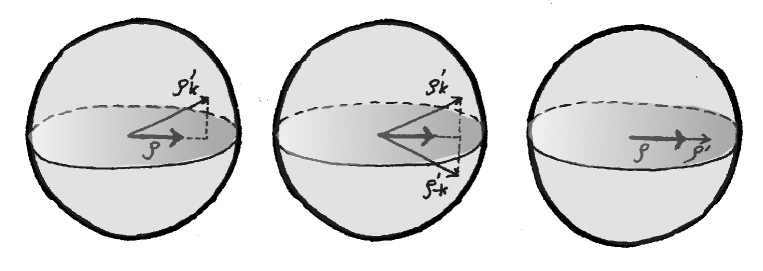
Figure 2.4: Schematic sketch of the $k$-symmetrization procedure.

We will refer to such a property as $k$-symmetry property of bradcasting maps and we showed that $k$-symmetry property is equivalent to the property of mapping equatorial states to equatorial states. Notice that a $k$-symmetric map is such that $r_{n,n^{\prime},k}^{jl}=r_{n,n^{\prime},-k}^{jl}$. The strategy to obtain broadcasting maps optimizing the reduced output state Bloch vector length is then to search for optimal maps within extremal maps and, once found the best one, to force $k$-symmetry on it. The procedure is shown in Fig. 2.4. On the left there are the equatorial mixed input state $\rho$ and the single-site reduced output $\rho^{\prime}_{k}$. Suppose such an output comes from an extremal map ${\mathcal{B}}_{k}$ described by $r_{n,n^{\prime},k}^{jl}$ elements. Notice that, by covariance, the projection of $\rho^{\prime}_{k}$ onto the equator is parallel with $\rho$. Consider now another map ${\mathcal{B}}_{-k}$, whose elements are equal to $\tilde{r}_{n,n^{\prime},k}^{jl}=r_{n,n^{\prime},-k}^{jl}$. Clearly, ${\mathcal{B}}_{-k}$ is a proper channel obeying all covariance and extremality constraints as ${\mathcal{B}}_{k}$. The output of ${\mathcal{B}}_{-k}$ is in sketched in the middle figure as $\rho^{\prime}_{-k}$. In order to have an equatorial output, we mix ${\mathcal{B}}_{k}$ and ${\mathcal{B}}_{-k}$ obtaining ${\mathcal{B}}=({\mathcal{B}}_{k}+{\mathcal{B}}_{-k})/2$ whose output $\rho^{\prime}=(\rho^{\prime}_{k}+\rho^{\prime}_{-k})/2$, by linearity, lies on the equator (see the picture on the right). Of course ${\mathcal{B}}$ is no more extremal, by construction. However, the figure of merit we are considering, namely, the length of the projection of the output Bloch vector onto the original one, does not change. In this sense, imposing $k$-symmetry does not affect optimality. Moreover, it is possible to prove that the $k$-symmetrized output $\rho^{\prime}$ has higher fidelity with the input $\rho$ (see Ref. [21])) than the tilted $\rho^{\prime}_{k}$ and $\rho^{\prime}_{-k}$.

Optimization

In Ref [21] it is proved that the channel optimizing the merit function

$$\mathfrak{F}=\operatorname{Tr}\left[\left(\sigma_{x}\otimes I^{M-1}\right)\ \Sigma\right],$$ (2.96)

for $x$-oriented input states $\rho=(I+r\sigma_{x})/2$, has $j_{l}=M/2$ for all $l$, and $k_{l}=0$, for $M-N$ even, while $k_{l}=\pm 1/2$ for $M-N$ odd. Hence, for $M-N$ even the optimal superbroadcaster is already $k$-symmetrized, whereas for $M-N$ odd we must equally mix the channels coming from $k_{l}=1/2$ and $k_{l}=-1/2$. In both cases, $r_{n,n^{\prime},k_{l}}^{j_{l},l}=1/d_{j_{l}}$, for all $n,n^{\prime},l$. At the end, the structure of the map ${\mathcal{B}}$ depends only on the parity of $M-N$, and not on the spectrum of $\rho$.

Figure 2.5: The plot shows the behaviour of the scaling factor $p^{N,N+1}(r)$ versus $r$, for $N$ ranges from 4 to 100 in steps of 8, in the phase-covariant case. Notice that there is a wide range of values of $r$ such that $p^{N,N+1}(r)>1$.

For $M-N$ even, the optimum scaling factor $p^{N,M}(r)$ is given by

$$p^{N,M}_{e}(r)=\frac{4}{Mr}\left(\frac{1-r^{2}}{4}\right)^{N/2}\sum_{l=l_{0}}^{N/2}d_{l}\sum_{n=-l}^{l}\left[\exp\left(J_{x}^{(l)}\log\frac{1+r}{1-r}\right)\right]_{n,n+1}\left[J_{x}^{(j)}\right]_{n,n+1},$$ (2.97)

while, for $M-N$ odd, it is

$$p^{N,M}_{o}(r)=\frac{4}{Mr}\left(\frac{1-r^{2}}{4}\right)^{N/2}\sum_{l=l_{0}}^{N/2}d_{l}\sum_{n=-l}^{l}\left[\exp\left(J_{x}^{(l)}\log\frac{1+r}{1-r}\right)\right]_{n,n+1}\left[J_{x}^{(j)}\right]_{n+1/2,n+3/2}.$$ (2.98)

In Fig. 2.5 there are the plots of $p^{N,N+1}(r)$ for $4\leq N\leq 100$ in steps of 8. As in the universal case, all curves, for $r\to 1$, go below one: indeed optimal phase-covariant cloning of pure states never achieves fidelity one, see Eq. (2.75). However, it is possible to see that phase-covariant superbroadcasting is more efficient than the universal one: superbroadcasting first emerges for $N=3$ ($N=4$ in the universal case) and achieves larger values of $p^{N,M}(r)$ for all $N$, $M$, and $r$.

Figure 2.6: Logarithmic plot of $(1-r^{*})$ versus $N$ in the phase-covariant case. The upper line refers to the case $M=\infty$ and shows a behaviour like $1/2N$. The lower line is for $M=N+1$ and goes like $2/(3N^{2})$.

In Fig. 2.6 there are the plots of $1-r^{*}(N,M)$, for $M=N+1$ and $M=\infty$, as done for the universal superbroadcaster. With good approximation, the two curves have power law $2/3N^{2}$ and $1/2N$, respectively, namely they go to zero faster than in the universal case, as expected.

Chapter 3 Realization of Quantum Devices

In the previous Chapter we explicitly wrote quantum operations coming out from an optimization procedure in a covariant setting. We gave such channels in terms of their Choi-Jamiołkowski operators (2.1). However, Choi-Jamiołkowski representation for quantum channels, even if very useful in dealing with semi-definite programming problems, turns out to be quite far from giving the physical “recipe” needed to realize the channel in a laboratory. In the following we will describe how to unitarily implement a given quantum channel, in terms of a unitary interaction between the system and an ancilla. In the first Section, we will provide, following Refs. [36, 37], a general method to work out a physical setting realizing a given channel. In the second part of the Chapter, we will show how this procedure works in the case of some of the channels discussed in Chapter 2.

3.1 Unitary dilations of a channel

Let us given a channel ${\mathcal{E}}:{\sf S}(\mathscr{H})\to{\sf S}(\mathscr{H})$. The task of this Section is to find an ancilla system $\mathscr{A}$, an ancilla pure state $|0\rangle$, and a unitary operator $U$ on $\mathscr{H}\otimes\mathscr{A}$, such that

$${\mathcal{E}}(\rho)=\operatorname{Tr}_{\mathscr{A}}\left[U(\rho\otimes|0\rangle\langle 0|)U^{\dagger}\right],$$ (3.1)

for all $\rho\in{\sf S}(\mathscr{H})$.

3.1.1 Stinespring dilation

Given a channel ${\mathcal{E}}$, the Stinespring representation [38] $(V,\mathscr{A})$ of ${\mathcal{E}}$ is a kind of “purification” of the channel ${\mathcal{E}}$, i. e.

$${\mathcal{E}}(\rho)=\operatorname{Tr}_{\mathscr{A}}\left[V\rho V^{\dagger}\right],$$ (3.2)

where $V$ is an isometry, i. e. $V^{\dagger}V=I$, from $\mathscr{H}$ to $\mathscr{H}\otimes\mathscr{A}$. The Stinespring representation is usually given for the dual channel (see Subsection 1.4.2) ${{\mathcal{E}}}^{\tau}:{\sf B}(\mathscr{H})\to{\sf B}(\mathscr{H})$ as

$${{\mathcal{E}}}^{\tau}(O)=V^{\dagger}(O\otimes I_{\mathscr{A}})V.$$ (3.3)

Let ${\mathcal{E}}(\rho)=\sum_{i}E_{i}\rho E_{i}^{\dagger}$ be a Kraus representation for ${\mathcal{E}}$. Consider now the operators from $\mathscr{H}$ to $\mathscr{H}\otimes\mathscr{A}$ defined as $E_{i}\otimes|i\rangle$, where $|i\rangle$ belongs to a set of orthonormal vectors in $\mathscr{A}$. The only trivial condition $\mathscr{A}$ must satisfy is $\mathsf{dim}\mathscr{A}\geq\sharp\{E_{i}\}$. Then, the sum

$$V=\sum_{i}E_{i}\otimes|i\rangle$$ (3.4)

is an isometry, since $V^{\dagger}V=\sum_{i}E_{i}^{\dagger}E_{i}=I_{\mathscr{H}}$, and realizes the channel ${\mathcal{E}}$ as in Eq. (3.2).

Remark 3.1.1

Notice that we did not make any assumption on the particular choice for the Kraus representation $\{E_{i}\}$ used to construct the Stinespring isometry $V$ in Eq. (3.4). When $\{E_{i}\}$ is the canonical Kraus decomposition and $\mathsf{dim}\mathscr{A}=\sharp\{E_{i}\}$, we will refer to such $V$ as the canonical Stinespring representation for ${\mathcal{E}}$, which clearly is the one minimizing the ancillary resources, i. e. the dimension of the ancilla system, needed to physically implement the channel.

3.1.2 Unitary dilation

From Stinespring form (3.2) the existence of a unitary interaction $U$ between $\mathscr{H}$ and $\mathscr{A}$ realizing the channel ${\mathcal{E}}$ is apparent, since every isometry $V$ from $\mathscr{H}$ to $\mathscr{H}\otimes\mathscr{A}$ can obviously be written as

$$V=U(I_{\mathscr{H}}\otimes|0\rangle),$$ (3.5)

where $U$ is a suitable unitary operator on $\mathscr{H}\otimes\mathscr{A}$ and $|0\rangle$ is a fixed normalized state of $\mathscr{A}$. Now, $|0\rangle$ is precisely the ancilla state such that

$${\mathcal{E}}(\rho)=\operatorname{Tr}_{\mathscr{A}}\left[U(\rho\otimes|0\rangle\langle 0|)U^{\dagger}\right].$$ (3.6)

While the existence of a realization $U$ for every channel is a well-established fact in the literature [8, 39], the problem of giving explicitly such interaction for a given channel can be very difficult. The general procedure given in Ref. [37] basically relies on a repeated Gram-Schmidt orthonormalizing algorithm applied to the column vectors of the Stinespring isometry $V$. In this way we are able to find additional $\mathsf{dim}\mathscr{H}\times(\mathsf{dim}\mathscr{A}-1)$ orthonormal vectors to append to $V$, completing it to a square matrix whose column vectors form an orthonormal basis for the composite system $\mathscr{H}\otimes\mathscr{A}$, i. e. to a unitary operator on $\mathscr{H}\otimes\mathscr{A}$. In the following Section, we will see that, in some fortunate cases, the channels optimized in Chapter 2 admit very simple Stinespring isometries, allowing us to explicitly write unitary operators realizing such channels in dimension $d$.

3.2 Explicit realizations

3.2.1 Universal NOT and cloning gates

Let us start from the optimal universal NOT-gate ${\mathcal{T}}$ derived in Subsection 2.4.2. The channel is completely described by the positive operator $R_{\mathcal{T}}$ in Eq. (2.53). In order to write ${\mathcal{T}}$ in its Stinespring form, we first have to obtain a Kraus decomposition for ${\mathcal{T}}$. This can be done by expanding $R_{\mathcal{T}}$ (see Section 2.1) as

$$\begin{split}R_{\mathcal{T}}&=\frac{2}{d+1}P_{S}^{(2)}=\frac{1}{d+1}(I+S)\\ &=\frac{1}{d+1}\sum_{m,n=0}^{d-1}(|m\rangle\langle m|\otimes|n\rangle\langle n|+|m\rangle\langle n|\otimes|n\rangle\langle m|)\\ &=\frac{1}{2(d+1)}\sum_{m,n=0}^{d-1}(|mn\rangle\!\rangle+|nm\rangle\!\rangle)(\langle\!\langle mn|+\langle\!\langle nm|)\\ &=\sum_{m,n=0}^{d-1}|M^{S}_{mn}\rangle\!\rangle\langle\!\langle M^{S}_{mn}|,\end{split}$$ (3.7)

where

$$M^{S}_{mn}=\frac{1}{\sqrt{2(d+1)}}(|m\rangle\langle n|+|n\rangle\langle m|).$$ (3.8)

One possible Kraus decomposition is then given by

$${\mathcal{T}}(\psi)=\sum_{m,n=0}^{d-1}M^{S}_{mn}\psi M^{S}_{mn}.$$ (3.9)

A Stinespring isometry $V$ such that ${\mathcal{T}}(\psi)=\operatorname{Tr}_{\mathscr{A}}\left[V\psi V^{\dagger}\right]$ is then

$$V=\sum_{m,n=0}^{d-1}M^{S}_{mn}\otimes|mn\rangle\!\rangle_{23},$$ (3.10)

where we chose $\mathscr{A}\equiv\mathscr{H}^{\otimes 2}$ as ancilla system. Summarizing, we wrote the optimal NOT-gate ${\mathcal{T}}$ by means of an isometry $V$ embedding the input system $\mathscr{H}$ into a composite tripartite system $\mathscr{H}\otimes\mathscr{H}\otimes\mathscr{H}$, in which the last two spaces represent the ancilla.

Tracing $V\psi V^{\dagger}$ over the last two spaces, we get the channel ${\mathcal{T}}$. What happens if we trace over different combinations of spaces? In fact, all three spaces are the same and there is no reason to consider one of them as the preferred system and the remaining ones as ancillae. Actually, tracing $V\psi V^{\dagger}$ over the first space, one obtains

$$\operatorname{Tr}_{1}\left[V\psi V^{\dagger}\right]=\frac{2}{d+1}P_{S}^{(2)}(I\otimes\psi)P_{S}^{(2)},$$ (3.11)

namely, the optimal $1\to 2$ universal cloning for pure states (see Eq. 2.50). This means that universal $1\to 2$ cloning and universal NOT-gate are intimately related and contextually appear on different branches (spaces) of the same physical setting. Such a coincidence has been experimentally exploited for qubits in Ref. [40] and theoretically analyzed and interpreted in generic dimension in Ref. [41]. Moreover, it is possible to prove that $\operatorname{Tr}_{3}\left[V\psi V^{\dagger}\right]$ optimally approximate the transformation $\psi\to\psi^{*}\otimes\psi$ for pure states. Notice that the cloning map is basis independent, whilst the transposition map depends on the choice of the basis, which is reflected by the choice of the particular Stinespring isometry $V$.

In Ref. [25] it is possible to find the explicit calculation deriving a unitary interaction and an ancilla state realizing at the same time optimal approximations of universal cloning and transposition. The unitary operator $U$ on $(\mathbb{C}^{d})^{\otimes 3}$ is

$$U=\sum_{p=0}^{d-1}V_{p,p}\otimes\langle p|\langle p|+\sum_{{p,q=0\atop p<q}}^{d-1}V_{p,q}^{(S)}\otimes\frac{\langle p|\langle q|+\langle q|\langle p|}{\sqrt{2}}+\sum_{{p,q=0\atop p<q}}^{d-1}V_{p,q}^{(A)}\otimes\frac{\langle p|\langle q|-\langle q|\langle p|}{\sqrt{2}}$$ (3.12)

where the three sets of isometries $\left\{V_{p,p}\right\}$, $\left\{V_{p,q}^{(S)}\right\}$, and $\left\{V_{p,q}^{(A)}\right\}$ from $\mathscr{H}$ to $\mathscr{H}^{\otimes 3}$ are defined as

$$\begin{split}&V_{p,p}=\sum_{k=0}^{d-1}|k\rangle|k\oplus p\rangle|k\oplus p\rangle\langle k\oplus p|,\\ &V_{p,q}^{(S)}=\frac{1}{\sqrt{2}}\sum_{k=0}^{d-1}|k\rangle(|k\oplus p\rangle|k\oplus q\rangle+|k\oplus q\rangle|k\oplus p\rangle)\langle k\oplus q|,\\ &V_{p,q}^{(A)}=\frac{1}{\sqrt{2}}\sum_{k=0}^{d-1}|k\rangle(|k\oplus p\rangle|k\oplus q\rangle-|k\oplus q\rangle|k\oplus p\rangle)\langle k\oplus q|.\end{split}$$ (3.13)

Preparing the ancilla state as

$$|\phi\rangle\!\rangle=\sqrt{\frac{2}{d+1}}P_{S}^{(2)}\sum_{r=0}^{d-1}|0\rangle|r\rangle,$$ (3.14)

the following identity holds

$$U(\psi\otimes|\phi\rangle\!\rangle\langle\!\langle\phi|)U^{\dagger}=V\psi V^{\dagger},$$ (3.15)

namely, the operator $U$ in Eq. (3.12) together with the ancilla state $|\phi\rangle\!\rangle$ in Eq. (3.14) provide a unitary dilation of the Stinespring isometry $V$ in Eq. (3.10), realizing optimal universal $1\to 2$ cloning as well as optimal universal transposition, depending on what we trace out after the interaction.

In the case $d=2$, we obtain the network model for universal qubit cloning of Ref. [42], with

$$U=\begin{pmatrix}1&0&0&0&0&0&0&0\\ 0&0&0&0&0&1&0&0\\ 0&0&0&0&0&0&1&0\\ 0&0&0&0&0&0&0&1\\ 0&0&0&1&0&0&0&0\\ 0&0&1&0&0&0&0&0\\ 0&1&0&0&0&0&0&0\\ 0&0&0&0&1&0&0&0\\ \end{pmatrix},$$ (3.16)

and $|\phi\rangle\!\rangle=\frac{1}{\sqrt{6}}(2|0\rangle|0\rangle+|0\rangle|1\rangle+|1\rangle|0\rangle)$.

3.2.2 Phase-covariant cloning and economical maps

In Subsection 2.5.1 we obtained the channel optimally achieving the multi-phase covariant $N\to M$ cloning transformation. The optimal channel has been described, as usual, by giving the corresponding $R_{\mathcal{C}}$ operator in Eq. (2.74). In the analyzed cases, i. e. when $M=N+kd$, where $k\in\mathbb{N}$ and $d$ is the dimension of the single copy system, $R_{\mathcal{C}}$ enjoys the relevent property of being rank-one. This implies that its canonical Kraus representation contains only one operator, and, to satisfy trace-preservation constraint (1.12), such an operator has to be an isometry. Therefore, the optimal multi-phase covariant $N\to M$ cloning machine ${\mathcal{C}}_{N,M}$, for $M=N+kd$, admits the very simple expression

$${\mathcal{C}}_{N,M}(\psi^{\otimes N})=V\psi^{\otimes N}V^{\dagger},$$ (3.17)

where $V:\mathscr{H}^{\otimes N}\to\mathscr{H}^{\otimes M}$ is an isometry acting as follows

$$V|\{n_{i}\}\rangle=|\{n_{i}+k\}\rangle,$$ (3.18)

using the compact notation introduced in Eq. (2.24).

This kind of isometric optimal channels attracted attention in the recent literature as economical transformations [43, 44, 45], in the sense that, in order to physically implement them, there is no need of discarding additional resources, i. e. ancillae. In fact, from the point of view of Stinespring representation, multi-phase covariant cloning is realizable as

$${\mathcal{C}}_{N,M}\left(\psi^{\otimes N}\right)=U\left(\psi^{\otimes N}\otimes|0\rangle\langle 0|^{\otimes(M-N)}\right)U^{\dagger},$$ (3.19)

namely, with respect to Eq. (3.6), there is no partial trace, and the resources needed are just the $(M-N)$ blank copies where convariantly distribute the information contained in $\psi^{\otimes N}$.

3.2.3 Phase-covariant NOT-gate

The optimal multi-phase conjugation map has been derived in Subsection 2.5.2 to be

$$R_{\mathcal{T}}=\sum_{i>j}b_{ij}(|ij\rangle+|ji\rangle)(\langle ij|+\langle ji|),$$ (3.20)

where $b_{ij}\geq 0$ are matrix elements of a null-diagonal symmetric bistochastic (NSB) matrix. In this case the map, for $d>2$, is not unitary or isometric as in the case of phase-covariant cloning. Moreover, the fact that in dimension $d\geq 4$ there exists a whole set of equally optimal maps—in one-to-one correspondence with NSB matrices—makes the problem of finding a physical realization much more difficult than in the two examples treated before, where the optimal map was unique. There are basically two paths one can follow: the first is to search for the most efficient realization, i. e. the one minimizing ancillary resources (in this case we will tipically single out one particular optimal phase-conjugation map achievable using less resources than the others); the second is to search for the most flexible realization, i. e. the one that spans as many as possible optimal maps by appropriately varying the “program” ancilla state and/or is more robust against noise (this second kind of realization will clearly require a higher dimensional ancilla system to encode a “fault-tolerant” program).

A good point to start with is the study of the structure of the set of optimal phase-conjugation channel, or, equivalently, of the set of NSB matrices. Such matrices form a convex set. On the other hand, every bistochastic matrix is a convex combination of permutation matrices—this is the content of the Birkhoff theorem [33]. The null-diagonal and symmetry constraints, however, force the convex set of NSB matrices to be strictly contained into the convex polyhedron of bistochastic matrices. This fact causes the extremal NSB matrices to eventually lie strictly inside the set of bistochastic matrices, generally preventing them from being permutations.

The geometrical study of the set of NSB matrices and its extremal points can shed some light on the unusual feature that there exist different “equally optimal” maps. The problem arises for dimension at least $d=4$. In this case the decomposition of the matrix $\{b_{ij}\}$ in Eq. (2.84) into extremal components is

$$\begin{split}\{b_{ij}\}&=p_{1}\begin{pmatrix}0&1&0&0\\ 1&0&0&0\\ 0&0&0&1\\ 0&0&1&0\end{pmatrix}+p_{2}\begin{pmatrix}0&0&1&0\\ 0&0&0&1\\ 1&0&0&0\\ 0&1&0&0\end{pmatrix}+p_{3}\begin{pmatrix}0&0&0&1\\ 0&0&1&0\\ 0&1&0&0\\ 1&0&0&0\end{pmatrix}\\ &=p_{1}B^{(1)}+p_{2}B^{(2)}+p_{3}B^{(3)},\end{split}$$ (3.21)

where $p_{1},p_{2},p_{3}\geq 0$ and $p_{1}+p_{2}+p_{3}=1$. A natural question is now which optimal maps can be achieved with minimal resources.

More explicitly, for $d=4$, we define three unitaries $U_{1}$, $U_{2}$ and $U_{3}$ on $\mathbb{C}^{4}\otimes\mathbb{C}^{2}$ as

$$U_{1}=\begin{pmatrix}T_{10}&T_{32}\vspace{0.2cm}\\ T_{32}&T_{10}\end{pmatrix},\quad U_{2}=\begin{pmatrix}T_{20}&T_{31}\vspace{0.2cm}\\ T_{31}&T_{20}\end{pmatrix},\quad U_{3}=\begin{pmatrix}T_{30}&T_{21}\vspace{0.2cm}\\ T_{21}&T_{30}\end{pmatrix},$$ (3.22)

where $T_{ij}=|i\rangle\langle j|+|j\rangle\langle i|$. Each of them realizes an extremal optimal multi-phase conjugation map (corresponding to $p_{k}=1$ in Eq. (3.21) for a given $k$), namely

$$\mathcal{T}^{(k)}_{4}(\rho)=\sum_{i>j}B^{(k)}_{ij}T_{ij}\rho T_{ij}=\operatorname{Tr}_{a}[U_{k}\;(\rho\otimes|0\rangle\langle 0|_{a})\;U_{k}^{\dagger}],$$ (3.23)

where $|0\rangle\langle 0|_{a}$ is a fixed qubit ancilla state. Hence extremal phase-conjugation maps for $d=4$ can be achieved with just a control qubit. Notice that the ancilla must not necessarily be in a pure state, and the optimal map is equivalently achieved for diagonal mixed ancilla state $\alpha|0\rangle\langle 0|_{a}+\beta|1\rangle\langle 1|_{a}$. By adding a control qutrit, we can now choose among any of the optimal maps using the controlled-unitary operator on $\mathbb{C}^{4}\otimes\mathbb{C}^{2}\otimes\mathbb{C}^{3}$

$$U=U_{1}\otimes|0\rangle\langle 0|+U_{2}\otimes|1\rangle\langle 1|+U_{3}\otimes|2\rangle\langle 2|.$$ (3.24)

Any optimal multi-phase conjugation map can now be written as

$$\mathcal{T}_{4}(\rho)=\operatorname{Tr}_{a,b}\left[U\;\left(\rho\otimes|0\rangle\langle 0|_{a}\otimes\sigma_{b}\right)\;U^{\dagger}\right]$$ (3.25)

where $\sigma_{b}$ is a generic density matrix on $\mathbb{C}^{3}$. By superimposing or mixing the three orthogonal states $\{|0\rangle,|1\rangle,|2\rangle\}$ of the qutrit we control the weights $p_{1},p_{2},p_{3}$ in Eq. (3.21) via the diagonal entries of $\sigma_{b}$. In other words, using a 6-dimensional ancilla it is possible to span the whole set of optimal maps.

Eqs. (3.22)-(3.25) can be generalized for higher even dimensions, with

$$\begin{split}&U_{k}=\sum_{i,j=0}^{\frac{d}{2}-1}T_{k\oplus 2i\oplus 2j,2i\oplus 2j}\otimes|i\rangle\langle j|,\qquad k=1,\dots,d-1,\\ &U=\sum_{k=1}^{d-1}U_{k}\otimes|k\rangle\langle k|,\\ &\mathcal{T}^{(k)}_{d}(\rho)=\operatorname{Tr}_{a}[U_{k}\;(\rho\otimes|0\rangle\langle 0|_{a})\;U_{k}^{\dagger}],\\ &\mathcal{T}_{d}(\rho)=\operatorname{Tr}_{a,b}\left[U\;\left(\rho\otimes|0\rangle\langle 0|_{a}\otimes\sigma_{b}\right)\;U^{\dagger}\right]\\ \end{split}$$ (3.26)

where $U_{k}$’s are unitary operators acting on $\mathbb{C}^{d}\otimes\mathbb{C}^{d/2}$, $U$ is a control-unitary operator on $\mathbb{C}^{d}\otimes\mathbb{C}^{d/2}\otimes\mathbb{C}^{d-1}$, $|0\rangle\langle 0|_{a}$ is a fixed $(d/2)$-dimensional pure state, and $\sigma_{b}$ is a generic $(d-1)$-dimensional density matrix. The minimum dimension of the ancilla space required to unitarily realize an optimal phase covariant transposition map is $d/2$, generalizing the result for $d=4$, for which just a qubit is needed (see Eq. (3.23)). On the other hand, to span the whole optimal maps set one needs a $(d-1)d/2$-dimensional ancilla.

Finally, notice that realization of multi-phase covariant transposition generally needs much less resources than realization of universal transposition: the minimum dimension $d/2$ of the ancilla space in the phase covariant case has to be compared with the dimension $d^{2}$ required in the universal case (3.14).

Chapter 4 The Role of Noise in Quantum Processes

In the previous Chapters we saw how to optimize transformations over quantum systems and how to realize them by means of physical interactions. Of course, processing of quantum systems requires a very high level of control during all steps of the experiment. On the other hand, noise—in the sense of uncontrollable interactions of the system with the sorroundings—is not always and completely avoidable: the only thing the experimenter can do is to reduce it in order to reach the desired level of confidence. This can be done by trying to directly control the environment, e. g. forcing it into a cavity, or by engineering states, interactions and measuring apparata robust with respect to the adopted model of noise.

In the following Sections we will deal with noise on measuring apparata and on states. While in the first part (review of Ref. [46]) we will face very general models of noise—basically, all non-unitary completely positive maps—in the second part (review of Ref. [47]) we will focus on decoherence of quantum states, proposing a novel correcting scheme retrieving classical information that the decoherence process made leak into the environment and exploiting such information to undo the noise.

4.1 Clean POVM’s

Let us given a general apparatus performing a measurement on quantum states. We know that the most general way to mathematically model it is by means of a POVM $\mathbf{P}$, see Section 1.3. Let us now think for a while we don’t know how the apparatus $\mathbf{P}$ works. It could be noisy at the input gate, that is, quantum states undergo some uncontrolled transformation ${\mathcal{E}}$ before being measured, and/or noisy at the output, the outcomes being, let’s say, shuffled before being read by the experimenter. The two situations are depicted in Fig. 4.1.

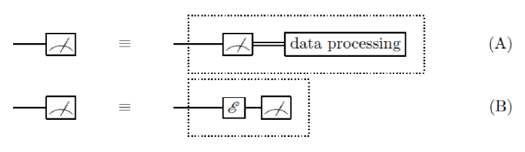
Figure 4.1: There are two ways of processing POVM’s: (A) the postprocessing of the output data and (B) the preprocessing of the input states by a quantum channel. The postprocessing is purely classical, whilst the preprocessing is quantum.

The question is the following: Do we have any condition on $\mathbf{P}$ that allows us to a priori affirm that $\mathbf{P}$ is “clean”, i. e. without noisy processing at the input and/or the output?

Clearly the point can be viewed from the complementary point of view: What kind of processings are possible on a given POVM? How does the apparatus change after such processings are performed?

4.1.1 Postprocessing of output data

The most general postprocessing of a POVM outcomes is a shuffling of with conditional probability $p(i|j)\geq 0$, corresponding to the mapping

$$Q_{i}=\sum_{j}p(i|j)P_{j},$$ (4.1)

where $\sum_{i}p(i|j)=1$, $\forall j$. To visualize the shuffling (4.1), it is useful to think to the POVM as a column of operators and $p(i|j)$ as a column-stochastic matrix

$$\begin{pmatrix}Q_{1}\\ Q_{2}\\ \vdots\\ Q_{n}\end{pmatrix}=\begin{pmatrix}p(1|1)&p(1|2)&\cdots&p(1|m)\\ p(2|1)&p(2|2)&\cdots&p(2|m)\\ \vdots&\vdots&\ddots&\vdots\\ p(n|1)&p(n|2)&\cdots&p(n|m)\\ \end{pmatrix}\begin{pmatrix}P_{1}\\ P_{2}\\ \vdots\\ P_{m}\end{pmatrix}.$$ (4.2)

Notice that postprocessing generally does not require that ${\mathbf{P}}$ and ${\mathbf{Q}}$ have the same cardinality. Relevant examples of postprocessing are:

1. identification of two outcomes, e. g. $j$ and $k$ are identified with the same outcome $l$, corresponding to $p(n|j)=p(n|k)=\delta_{ln}$;

2. permutation $\pi$ of outcomes, corresponding to $p(\pi(j)|k)=\delta_{jk}$.

When two POVM’s ${\mathbf{P}}$ and ${\mathbf{Q}}$ are connected by a mapping of the form (4.1) for some conditional probability $p(i|j)$ we will write ${\mathbf{P}}\succ_{p}{\mathbf{Q}}$, and say that the POVM ${\mathbf{P}}$ is cleaner under postprocessing—postprocessing cleaner, for short—than the POVM ${\mathbf{Q}}$. It is possible to prove that the relation $\succ_{p}$ is a pseudo-ordering, hence an equivalence relation under postprocessing can be defined as follows

Definition 4.1.1

The POVM’s ${\mathbf{P}}$ and ${\mathbf{Q}}$ are postprocessing equivalent—in symbols ${\mathbf{P}}\simeq_{p}{\mathbf{Q}}$—if and only if both relations ${\mathbf{P}}\succ_{p}{\mathbf{Q}}$ and ${\mathbf{Q}}\succ_{p}{\mathbf{P}}$ hold.

We are now in position to define cleanness under postprocessing, namely

Definition 4.1.2

A POVM ${\mathbf{P}}$ is postprocessing clean if and only if for any POVM ${\mathbf{Q}}$ such that ${\mathbf{Q}}\succ_{p}{\mathbf{P}}$, then also ${\mathbf{P}}\succ_{p}{\mathbf{Q}}$ holds, namely ${\mathbf{P}}\simeq_{p}{\mathbf{Q}}$.

The complete characterization of cleanness under postprocessing (classical) is given by the following theorem (see Refs. [46, 48])

Theorem 4.1.3 (postprocessing)

A POVM ${\mathbf{P}}$ is postprocessing clean if and only if it is rank-one.

This means that if a POVM is rank-one, we are sure that it does not have a hidden noisy postprocessing at the output. Viceversa, the Theorem says that it is not possible to obtain the statistics of a rank-one POVM by classically postprocessing the outcomes of a higher rank POVM.

4.1.2 Preprocessing of input states

A preprocessing ${\mathcal{E}}$ of input states induces naturally a dual channel ${{\mathcal{E}}}^{\tau}$ acting on the POVM itself, as seen in Subsection 1.4.2. Hence, we will write

$${\mathbf{P}}\succ{\mathbf{Q}}$$ (4.3)

and say that the POVM ${\mathbf{P}}$ is preprocessing cleaner than ${\mathbf{Q}}$, if and only if there exists a channel—i. e. a trace-preserving, completely positive map ${\mathcal{E}}$—such that $Q_{i}={{\mathcal{E}}}^{\tau}(P_{i})$, $\forall i$, or, equivalently ${\mathbf{Q}}={{\mathcal{E}}}^{\tau}({\mathbf{P}})$, for short. It is possible to prove that the relation $\succ$ is a pseudo-ordering, hence an equivalence relation under preprocessing can be defined as follows

Definition 4.1.4

The POVM’s ${\mathbf{P}}$ and ${\mathbf{Q}}$ are preprocessing equivalent—in symbols ${\mathbf{P}}\simeq{\mathbf{Q}}$—if and only if both relations ${\mathbf{P}}\succ{\mathbf{Q}}$ and ${\mathbf{Q}}\succ{\mathbf{P}}$ hold.

We are now in position to define cleanness under preprocessing, namely

Definition 4.1.5

A POVM ${\mathbf{P}}$ is preprocessing clean if and only if for any POVM ${\mathbf{Q}}$ such that ${\mathbf{Q}}\succ{\mathbf{P}}$, then also ${\mathbf{P}}\succ{\mathbf{Q}}$ holds, namely ${\mathbf{P}}\simeq{\mathbf{Q}}$.

From the above definition, it turns out that a POVM is preprocessing clean if and only if, whenever a noisy preprocessing acts, its action on the POVM can be perfectly inverted. Now, a result by Wigner tells that a channel admits an inverse channel (i. e. it is physically invertible) if and only if such a channel is actually unitary. A question arises: Does cleanness property define an interesting structure in the set of POVM’s? Or will we find that invertible preprocessings are just unitary (i. e. trivial) preprocessings? Generally, this is not the case, because we want the action of the noise to be invertible only on a fixed POVM, not on all ${\sf B}(\mathscr{H})$.

For qubits, however, preprocessing-equivalence coincides with unitary-equivalence

Theorem 4.1.6 (qubits)

For two-level systems ${\mathbf{P}}\simeq{\mathbf{Q}}$ if and only if there exists a unitary operator $U$ such that ${\mathbf{P}}=U^{\dagger}{\mathbf{Q}}U$.

In higher dimensions the counterexample is given implicitly by the following Theorem regarding effects (two-outcomes POVM’s, see Section 1.3)

Theorem 4.1.7 (effects)

Let ${\mathbf{P}}=\{P,I-P\}$ and ${\mathbf{Q}}=\{Q,I-Q\}$ be two effects. Then ${\mathbf{P}}\simeq{\mathbf{Q}}$ if and only if $\lambda_{M}(P)=\lambda_{M}(Q)$ and $\lambda_{m}(P)=\lambda_{m}(Q)$, where $\lambda_{m}(O)$ ($\lambda_{M}(O)$) is the minimum (maximum) eigenvalue of $O$.

Since necessary and sufficient condition for preprocessing-equivalence of two effects is that they have the same spectral width, ragardless of the spectrum itself, it is clear that there exist preprocessing-equivalent effects which are not unitarily equivalent (otherwise they should have the same spectrum as a whole). It is also clear that, for dimension $d=2$, the spectrum is completely determined by the spectral width, whence unitary-equivalence.

Besides effects, the other case in which we have a complete characterization of preprocessing clean POVM’s is the following

Theorem 4.1.8 (observables)

For number of outcomes $n\leq d$, the set of preprocessing clean POVM’s coincides with the set of observables.

This result is interesting since it provides an operational approach, alternative to the axiomatic one given by von Neumann, to define what are the observables in quantum theory. Here, just by introducing the cleanness pseudo-ordering, we singled out the set of observables, as the only clean POVM’s with numer of outcomes less or equal to the dimension of the Hilbert space—in this sense, they are the only clean “classical” POVM’s.

When the numbers of outcomes gets larger than the dimension of the Hilbert space, the structure introduced by the preprocessing pseudo-ordering on the convex set of POVM’s becomes more complicated, and we have just partial results. For example, we can prove that rank-one POVM’s are not only postprocessing clean, but also preprocessing clean

Theorem 4.1.9 (rank-one)

Rank-one POVM’s are preprocessing clean.

Notice that cleanness under preprocessing and extremality are properties completely unrelated. Consider, e. g., the following rank-one POVM

$$\frac{1}{2}|1\rangle\langle 1|,\frac{1}{2}|1\rangle\langle 1|,|2\rangle\langle 2|,\dots,|d\rangle\langle d|.$$ (4.4)

The redundantly doubled outcome $|1\rangle\langle 1|$ suggests at first sight that such a POVM cannot be extremal, namely, it cannot be the solution of any optimization problem. In this sense, such POVM “is not good”. However, being rank-one, it is clean under both preprocessing and postprocessing.

4.1.3 Positive maps

Since now, we introduced two pseudo-orderings on the set of POVM’s, the preprocessing ordering $\succ$, and the postprocessing ordering $\succ_{p}$. In this Subsection, we will introduce two additional relations which can be established among POVM’s, namely

Definition 4.1.10 (positive preprocessing)

We write ${\mathbf{P}}\gg{\mathbf{Q}}$ and say that ${\mathbf{P}}$ is cleaner than ${\mathbf{Q}}$ under positive preprocessing, if and only if there exists a positive (non necessarily completely positive) map ${\mathcal{P}}$ such that ${\mathbf{Q}}={\mathcal{P}}({\mathbf{P}})$.

Definition 4.1.11 (range-inclusion)

We write ${\mathbf{P}}\supset_{r}{\mathbf{Q}}$ and say that ${\mathbf{P}}$ range-includes ${\mathbf{Q}}$, if and only if ${\sf Rng}({\mathbf{Q}})\subseteq{\sf Rng}({\mathbf{P}})$, where the range of a POVM is defined in Definition 1.3.1.

We simply have the following hierarchy of relations

$${\mathbf{P}}\succ{\mathbf{Q}}\quad\Longrightarrow\quad{\mathbf{P}}\gg{\mathbf{Q}}\quad\Longrightarrow\quad{\mathbf{P}}\supset_{r}{\mathbf{Q}}.$$ (4.5)

The converse is not always true. However, we have some results providing sufficient conditions for which some of the relations in Eq. (4.5) can be inverted. Proofs are very technical and can be found in Ref. [46]. Here we just give the statements.

Theorem 4.1.12

Consider two POVM’s ${\mathbf{P}}$ and ${\mathbf{Q}}$ with the same number of outcomes. Then the following statements are equivalent:

1. ${\mathbf{P}}\supset_{r}{\mathbf{Q}}$

2. There is a (unique) positive map ${\mathcal{E}}:{\sf Span}({\mathbf{P}})\to{\sf Span}({\mathbf{Q}})$ with ${\mathcal{E}}({\mathbf{P}})={\mathbf{Q}}$.

Notice that point (2) does not say that ${\mathbf{P}}\gg{\mathbf{Q}}$, since the positive map is defined only from ${\sf Span}({\mathbf{P}})$ to ${\sf Span}({\mathbf{Q}})$, and generally cannot be extended to a positive map on all ${\sf B}(\mathscr{H})$. The following Theorems describe some situations in which it possible to extend the map ${\mathcal{E}}$ to a positive map over all ${\sf B}(\mathscr{H})$.

Theorem 4.1.13

Consider two POVM’s ${\mathbf{P}}$ and ${\mathbf{Q}}$ with the same number of outcomes. Then the following statements are equivalent:

1. ${\mathbf{P}}\succ{\mathbf{Q}}$

2. There is an informationally complete POVM $\mathbf{M}$ such that ${\mathbf{P}}\otimes\mathbf{M}\supset_{r}{\mathbf{Q}}\otimes\mathbf{M}$.

3. ${\mathbf{P}}\otimes\mathbf{M}\supset_{r}{\mathbf{Q}}\otimes\mathbf{M}$ holds for all POVM’s $\mathbf{M}$.

Theorem 4.1.14 (abelian POVM)

Consider two POVM’s ${\mathbf{P}}$ and ${\mathbf{Q}}$ with the same number of outcomes. Let ${\mathbf{Q}}$ be abelian, namely $Q_{i}Q_{j}=Q_{j}Q_{i}$ for all $i,j$. Then ${\mathbf{P}}\supset_{r}{\mathbf{Q}}$ $\Longrightarrow$ ${\mathbf{P}}\succ{\mathbf{Q}}$, and Eq. (4.5) becomes a chain of equivalences.

4.2 Inverting decoherence

We will now focus our attention on a particularly nasty preprocessing of input states, namely on decoherence. Decoherence is universally considered, on one side, as the major practical limitation for communication and processing of quantum information. On the other side, decoherence yields the key concept to explain the transition from quantum to classical world [49] due to the uncontrolled and unavoidable interactions with the environment. Great effort in the literature has been devoted to combat the effect of decoherence by engineering robust encoding-decoding schemes. Some authors have recently addressed a different approach to undo quantum noises by extracting classical information from the environment [50] and exploiting it as an additional amount of side information useful to improve quantum communication performances [51].

The recovery of quantum coherence from the environment is often a difficult task, e. g. when the environment is “too big” to be controlled, as for spontaneous emission of radiation. By regaining control on the environment the recovery can sometimes be actually accomplished, for example by keeping the emitted radiation inside a cavity. However, in some cases, the full recovery of quantum coherence becomes impossible even in principle, namely even when one has complete access to the environment. This naturally leads us to pose the following question: in which physical situations is possible to perfectly recover quantum coherence by monitoring the environment?

4.2.1 Convex structure of decoherence maps

A completely decohering evolution asymptotically cancels any quantum superposition when reaching the stationary state, making any state diagonal in some fixed orthonormal basis—the basis depending on the particular system-environment interaction. In the Heisenberg picture we say that such a completely decohering evolution asymptotically maps the whole algebra of quantum observables into a “maximal classical algebra”, that is a maximal set of commuting—namely jointly measureable—observables. Let’s denote by ${\mathfrak{A}}_{q}$ the “quantum algebra” of all bounded operators ${\sf B}(\mathscr{H})$ on the finite dimensional Hilbert space $\mathscr{H}$, and by ${\mathfrak{A}}_{c}$ the “classical algebra”, namely any maximal Abelian subalgebra ${\mathfrak{A}}_{c}\subset{\mathfrak{A}}_{q}$. Clearly, all operators in ${\mathfrak{A}}_{c}$ can be jointly diagonalized on a common orthonormal basis, which in the following will be denoted as $\mathbf{b}=\{|k\rangle|k=1,\dots,d\}$. Then, the classical algebra ${\mathfrak{A}}_{c}$ is also the linear span of the one-dimensional projectors $|k\rangle\langle k|$, whence ${\mathfrak{A}}_{c}$ is a $d$-dimensional vector space. According to the above general framework, we call (complete) decoherence map a completely positive identity-preserving (i. e. trace-preserving in the Schrödinger picture, see Subsection 1.4.2) map ${{\mathcal{E}}}^{\tau}$ which asymptotically maps any observable $O\in{\mathfrak{A}}_{q}$ to a corresponding “classical observable” in ${\mathfrak{A}}_{c}$, namely such that the limit $\lim_{n\to\infty}({{\mathcal{E}}}^{\tau})^{n}(O)$ exists and belongs to the classical algebra ${\mathfrak{A}}_{c}$ for any $O\in{\mathfrak{A}}_{q}$. Here we denote with $({{\mathcal{E}}}^{\tau})^{n}$ the $n$-th iteration of the map ${\mathcal{E}}$, implicitly assuming markovian evolution.

It is easy to see that the set of decoherence maps is convex. The following Theorem shows that such maps enjoy a remarkably simple form:

Theorem 4.2.1 (Schur form)

A map ${{\mathcal{E}}}^{\tau}$ preserves all elements of the maximal classical algebra ${\mathfrak{A}}_{c}$ if and only if it has the form

$${{\mathcal{E}}}^{\tau}(O)=\xi\circ O,$$ (4.6)

$A\circ B$ denoting the Schur product of operators $A$ and $B$, i. e. $A\circ B\equiv\sum_{k,l=1}^{d}A_{kl}B_{kl}|k\rangle\langle l|$, $\{A_{kl}\}$ and $\{B_{kl}\}$ being the matrix elements of $A$ and $B$ in the basis $\mathbf{b}$, and $\xi_{kl}$ being a correlation matrix, i.e. a positive semidefinite matrix with $\xi_{kk}=1$ for all $k=1,\dots,d$.

Theorem 4.2.1 states a linear correspondence between maps preserving ${\mathfrak{A}}_{c}$ and correlation matrices, whence the two sets share the same convex structure. Then the map is extremal if and only if its correlation matrix is extremal.

Since now we dealt with the dual map ${{\mathcal{E}}}^{\tau}$ on bounded operators. The action of a decoherence map on quantum states is given in Schrödinger picture by

$${\mathcal{E}}(\rho)=\xi^{T}\circ\rho,$$ (4.7)

where $T$ denotes transposition with respect to the basis $\mathbf{b}$ (also $\xi^{T}$ is a correlation matrix, hence in the following, we will drop the symbol $T$ at the exponent). As a consequence, one has exponential decay of the off-diagonal elements of $\rho$, since $\left|[{\mathcal{E}}^{n}(\rho)]_{kl}\right|=|\xi_{kl}|^{n}\cdot|\rho_{kl}|$. In other words, any initial state $\rho$ decays exponentially towards the completely decohered state

$$\rho_{\infty}\equiv\sum_{k}\rho_{kk}|k\rangle\langle k|.$$ (4.8)

In Ref. [47], it is proved the following

Lemma 4.2.2

A map ${\mathcal{E}}$ is an extremal decoherence map if and only if it is extremal in the set of all maps.

As a consequence of Lemma 4.2.2, the convex structure of decoherence maps can be obtained by application of the well known Choi Theorem [15], which states that the canonical Kraus operators $\{E_{i}\}$, $1\leq i\leq r$, of every extremal map are such that their products $\{E_{i}^{{\dagger}}E_{j}\}$, $1\leq i,j\leq r$, are linearly independent. A relevant consequence of this characterization is the following

Theorem 4.2.3

If ${\mathcal{E}}$ is an extremal decoherence map, then $r\leq\sqrt{d}$. For qubits and qutrits any decoherence map is then random-unitary.

This means that for qubits and qutrits extremal decoherence maps are unitary maps, since they admits a Kraus representation containing only one operator. Hence, for qubits and qutrits, every decoherence map can be written as

$${\mathcal{E}}(\rho)=\sum_{i}p_{i}U_{i}\rho U_{i}^{\dagger},$$ (4.9)

for some commuting unitary operators $U_{i}\in{\mathfrak{A}}_{c}$ and probability distribution $p_{i}$.

4.2.2 Correcting decoherence by measuring the environment

In Ref. [50] it is shown that the only channels that can be perfectly inverted by monitoring the environment are the random-unitary ones. Therefore, it follows that one can perfectly correct any decoherence map for qubits and qutrits by monitoring the environment. The correction is achieved by retrieving the index $i$ in Eq. (4.9) via a measurement on the environment, and then by applying the inverse of the unitary transformation $U_{i}$ on the system. Therefore, the random-unitary map simply leaks $H(p_{i})$ bits of classical information into the environment ($H$ denoting the Shannon entropy), and the effects of decoherence can be completely eliminated by recovering such classical information, without any prior knowledge about the input state. The fact that decoherence maps are necessarily random-unitary is true only for qubits and qutrits. A counterexample in dimension $d=4$ can be found in Ref. [47]. Such extremal decoherence maps with $r\geq 2$ represent a process which is fundamentally different from the random unitary one, corresponding to a leak of quantum information from the system to the environment, information that cannot be perfectly recovered from the environment [50].

Now we address the problem of estimating the amount of classical information needed in order to invert a random-unitary decoherence map. If the environment is initially in a pure state, say $|0\rangle_{e}$, a useful quantity to deal with is the so-called entropy exchange [52] $S_{\textrm{ex}}$ defined as

$$S_{\textrm{ex}}(\rho)=S(\sigma_{e}^{\rho}),$$ (4.10)

where $\sigma_{e}^{\rho}$ is the reduced environment state after the interaction with the system in the state $\rho$, and $S(\rho)=-\operatorname{Tr}[\rho\log\rho]$ is the von Neumann entropy. In the case of initially pure environment, the entropy exchange depends only on the map ${\mathcal{E}}$ and on the input state of the system $\rho$, regardless of the particular system-environment interaction chosen to model ${\mathcal{E}}$. It quantifies the information flow from the system to the environment and, for all input states $\rho$, one has the bound [52] $|S({\mathcal{E}}(\rho))-S(\rho)|\leq S_{\textrm{ex}}(\rho)$, namely the entropy exchange $S_{\textrm{ex}}$ bounds the entropy production at each step of the decoherence process.

In order to explicitly evaluate the entropy exchange for a decoherence process, we can then exploit a particular model interaction between system and environment. This can be done noticing that it is always possible to write $\xi_{kl}=\langle e_{l}|e_{k}\rangle$ for a suitable set of normalized vectors $\{|e_{k}\rangle\}$. Then, the map ${\mathcal{E}}(\rho)=\xi\circ\rho$ can be realized as ${\mathcal{E}}(\rho)=\operatorname{Tr}_{e}[U(\rho\otimes|0\rangle\langle 0|_{e})U^{\dagger}]$, where the unitary interaction $U$ gives the transformation

$$U|k\rangle\otimes|0\rangle_{e}=|k\rangle\otimes|e_{k}\rangle,$$ (4.11)

whence the final reduced state of the environment is $\sigma_{e}^{\rho}=\sum_{k}\rho_{kk}|e_{k}\rangle\langle e_{k}|$. Then, in order to evaluate $S_{\textrm{ex}}$ for a decoherence map ${\mathcal{E}}(\rho)=\xi\circ\rho$, it is possible to bypass the evaluation of the states $|e_{i}\rangle$ of the environment, using the formula

$$S_{\textrm{ex}}(\rho)=S(\sqrt{\rho_{\infty}}\xi\sqrt{\rho_{\infty}}),$$ (4.12)

which follows immediately from the fact that $\sqrt{\rho_{\infty}}\xi\sqrt{\rho_{\infty}}$, and $\sigma_{e}^{\rho}$ are both reduced states of the same bipartite pure state $\sum_{i}\sqrt{\rho_{ii}}|i\rangle|e_{i}\rangle$.

Notice that the unitary interaction $U$ in Eq. (4.11) generalizes the usual form considered for quantum measurements [4], with the quantum system interacting with a pointer, which is left in one of the (nonorthogonal) states $\{|e_{k}\rangle\}$. The more the pointer states are “classical”—i. e. distinguishable—the larger is the entropy exchange, whence the faster is the decoherence process. In the limit of orthogonal states, decoherence is istantaneous, i. e. ${\mathcal{E}}(\rho)=\rho_{\infty}$.

When a map can be inverted by monitoring the environment—i. e. in the random-unitary case—the entropy exchange $S_{\textrm{ex}}(I/d)$ provides a lower bound to the amount of classical information that must be collected from the environment in order to perform the correction scheme of Ref. [50]. In fact, assuming a random-unitary decomposition (4.9) and using the formula [52] $S_{\textrm{ex}}(\rho)=S\left(\sum_{i,j}\sqrt{p_{i}p_{j}}\operatorname{Tr}[U_{i}\rho U_{j}^{{\dagger}}]|i\rangle\langle j|\right)$, we obtain

$$S_{\textrm{ex}}(I/d)\leq H(p_{i}).$$ (4.13)

The inequality comes from the fact that the diagonal entries of a density matrix are always majorized by its eigenvalues [33], and it becomes equality if and only if $\operatorname{Tr}[U_{i}U_{j}^{{\dagger}}]/d=\delta_{ij}$, i. e. the map admits a random-unitary decomposition with orthogonal unitary operators. Moreover, from Eq. (4.12) we have $S_{\textrm{ex}}(I/d)=S(\xi/d)$.

In Ref. [47], it is proved that, for qubits, $S(\xi/2)$ quantifies exactly the minimum amount of classical information which must be extracted from the environment, while, for dimension $d>2$, the bound in Eq. (4.13) is generally strict and a counterexample is given for dimension $d=3$. Notice that the same decoherence map may be obtainable by different random-unitary decompositions with different probability distributions $\{p_{i}\}$, corresponding to different values of the information $H(p_{i})$. However, for qubits it is always possible to perform a suitable measurement on the environment and to invert the decoherence map retrieving the minimal amount of information from the environment, namely $S(\xi/2)$. For example, consider the so-called random phase-kick model [53] for decoherence of qubits

$${\mathcal{E}}(\rho)=\frac{1}{\sqrt{4\pi\lambda}}\int_{-\infty}^{+\infty}e^{i\theta\sigma_{z}/2}\rho e^{-i\theta\sigma_{z}/2}e^{-\theta^{2}/4\lambda}\textrm{d}\theta,$$ (4.14)

which can be rewritten as

$${\mathcal{E}}(\rho)=\xi\circ\rho,\qquad\xi=\begin{pmatrix}1&e^{-\lambda}\\ e^{-\lambda}&1\end{pmatrix}.$$ (4.15)

From Eq. (4.14), one could infer that the amount $S$ of classical information that must be extracted from the environment is equal to the differential entropy of the gaussian probability density according to which the system is random phase-kicked, namely (see Ref. [54])

$$S\left(\frac{1}{\sqrt{4\pi\lambda}}e^{-\theta^{2}/4\lambda}\right)=\frac{1}{2}\log 4\pi e\lambda,$$ (4.16)

growing logarithmically with $\lambda$. This is actually not correct, since the minimum amount of classical information needed is

$$S=-p\log_{2}p-(1-p)\log_{2}(1-p),\qquad p=\frac{1-e^{-\lambda}}{2}.$$ (4.17)

In fact, $\xi/2$ in Eq. (4.15) can be simply diagonalized and has eigenvalues $\left\{\frac{1-e^{-\lambda}}{2},\frac{1+e^{-\lambda}}{2}\right\}$.

Figure 4.2: The amount of classical information $S$, expressed in bits, leaking into the environment at every application of the random phase-kick model of decoherence for qubits, as function of the parameter $\lambda$, see Eqs. (4.14) and (4.15). $S$ tends to the limit value of 1 bit, since every qubit decoherence map can be written as a random-unitary process involving only two unitaries (see the footnote in the previous page).

In Figure 4.2 there is the plot of the amount of classical information $S$ in Eq. (4.17) as a function of the parameter $\lambda$ modelling the decoherence rate in Eqs. (4.14) and (4.15). The curve tends to the finite limit of one bit, contrarily to what happens in Eq. (4.16).

List of Publications

• F Buscemi, G M D’Ariano, C Macchiavello, and P Perinotti,
  Optimal superbroadcasting maps of mixed qubit states,
  in preparation

• F Buscemi, G M D’Ariano, M Keyl, P Perinotti, and R F Werner,
  Clean positive operator valued measures,
  J. Math. Phys. 46, 082109 (2005)

• F Buscemi, G Chiribella, and G M D’Ariano,
  Inverting quantum decoherence by classical feedback from the environment,
  Phys. Rev. Lett. 95, 090501 (2005)

• F Buscemi, G M D’Ariano, and C Macchiavello,
  Optimal Time-Reversal of Multi-phase Equatorial States,
  pre-print on quant-ph/0504016

• F Buscemi, G M D’Ariano, and C Macchiavello,
  Economical Phase-Covariant Cloning of Qudits,
  Phys. Rev. A 71, 042327 (2005)

• F Buscemi, G M D’Ariano, and P Perinotti,
  There exist non orthogonal quantum measurements that are perfectly repeatable,
  Phys. Rev. Lett. 92, 070403 (2004)

• F Buscemi, G M D’Ariano, and M F Sacchi,
  Physical realizations of quantum operations,
  Phys. Rev. A 68, 042113 (2003)

• F Buscemi, G M D’Ariano, P Perinotti, and M F Sacchi,
  Optimal realization of the transposition maps,
  Phys. Lett. A 314, 374 (2003)

• F Buscemi, G M D’Ariano, and M F Sacchi,
  Unitary realizations of the ideal phase measurement,
  Phys. Lett. A 312, 315 (2003)

References

- [1] A S Holevo, Probabilistic and Statistical Aspects of Quantum Theory (North-Holland Publishing Company, 1982).
- [2] A S Holevo, Lectures on Statistical Structure of Quantum Theory (1999).
- [3] P Busch, P Mittelstaedt, and P Lahti, The Quantum Theory of Measurement (Springer-Verlag, 1991).
- [4] J von Neumann, Mathematical Principles of Quantum Mechanics (Princeton University Press, 1955)
- [5] G Lüders, Ann. Phys. 8, 322 (1951). Translated in K A Kirkpatrick, quant-ph/0403007.
- [6] K Kraus, States, Effects, and Operations: Fundamental Notions in Quantum Theory, Lect. Notes Phys. 190, (Springer-Verlag, 1983).
- [7] E B Davies and J T Lewis, Commun. Math. Phys. 17, 239 (1970).
- [8] M Ozawa, J. Math. Phys. 5, 848 (1984).
- [9] M Ozawa, in Quantum Communication, Computing, and Measurement, ed. by P Tombesi and O Hirota, 3, 97 (Kluwer/Plenum, 2001). Available on quant-ph/0107090.
- [10] F Buscemi, G M D’Ariano, and M F Sacchi, Phys. Lett. A 312, 315 (2003). Available on quant-ph/0304071.
- [11] C W Helstrom, Quantum Detection and Estimation Theory (Academic Press, 1976).
- [12] F Buscemi, G M D’Ariano, and P Perinotti, Phys. Rev. Lett. 92, 070403 (2004). Available on quant-ph/0310041.
- [13] see, for example, P R Halmos, A Hilbert Space Problem Book (Springer-Verlag, 1982).
- [14] A Jamiołkowski, Rep. Math. Phys. 3, 275 (1972).
- [15] M-D Choi, Lin. Alg. Appl. 10, 285 (1975).
- [16] G M D’Ariano and P Lo Presti, Phys. Rev. A 64, 042308 (2001). Available on quant-ph/0101100.
- [17] D P Zhelobenko, Compact Lie Groups and Their Representations (American Mathematical Society, 1973).
- [18] see, for example, H F Jones, Groups, Representations and Physics (Institute of Physics Publishing, 1996).
- [19] see, for example, A Messiah, Quantum Mechanics (John Wiley and Sons, 1958).
- [20] J I Cirac, A K Ekert, and C Macchiavello, Phys. Rev. Lett. 82, 4344 (1999). Available on quant-ph/9812075.
- [21] F Buscemi, G M D’Ariano, C Macchiavello, and P Perinotti, in preparation.
- [22] R F Werner, Phys. Rev. A 58, 1827 (1998). Available on quant-ph/9804001.
- [23] W K Wootters and W H Zurek, Nature 299, 802 (1982); H P Yuen, Phys. Lett. A 113, 405 (1986).
- [24] seminal papers in this direction are: V Bužek and M Hillery, Phys. Rev. A 54, 1844 (1996), avail. on quant-ph/9607018; N Gisin and S Massar, Phys. Rev. Lett. 79, 2153 (1997), avail. on quant-ph/9705046; D Bruß, A Ekert, and C Macchiavello, Phys. Rev. Lett. 81, 2598 (1998), avail. on quant-ph/9712019.
- [25] F Buscemi, G M D’Ariano, P Perinotti, and M F Sacchi, Phys. Lett. A 314, 374 (2003). Available on quant-ph/0304175.
- [26] V Buzek, M Hillery, and R F Werner, Phys. Rev. A 60, R2626 (1999). Available on quant-ph/9901053.
- [27] D Bruß and C Macchiavello, Phys. Lett. A 253, 249 (1999). Available on quant-ph/9812016.
- [28] H Barnum, C M Caves, C A Fuchs, R Jozsa, and B Schumacher, Phys. Rev. Lett. 76, 2818 (1996). Available on quant-ph/9511010.
- [29] G M D’Ariano, C Macchiavello, and P Perinotti, to appear on Phys. Rev. Lett. Available on quant-ph/0506251.
- [30] S Bandyopadhyay, P O Boykin, V Roychowdhury, and F Vatan, Algorithmica 34, 512 (2002). Available on quant-ph/0103162.
- [31] F Buscemi, G M D’Ariano, and C Macchiavello, Phys. Rev. A 71, 042327 (2005). Available on quant-ph/0407103.
- [32] F Buscemi, G M D’Ariano, and C Macchiavello, preprint on quant-ph/0504016.
- [33] R Bhatia, Matrix Analysis, Springer Graduate Texts in Mathematics, Vol. 169 (Springer, 1996).
- [34] C Macchiavello, Phys. Rev. A 67, 062302 (2003). Available on quant-ph/0304126.
- [35] C-K Li and B-S Tam, SIAM J. Matrix Anal. Appl. 15, 903 (1994).
- [36] F Buscemi, Degree Thesis, (2002). Available (in italian) at URL http://www.qubit.it/~buscemi/notes/thesis.pdf.
- [37] F Buscemi, G M D’Ariano, and M F Sacchi, Phys. Rev. A 68, 042113 (2003). Available on quant-ph/0305180.
- [38] W F Stinespring, Proc. Am. Math. Soc. 6, 211 (1955).
- [39] K Kraus, in Foundations of Quantum Mechanics and Ordered Linear Spaces, Vol. 29 of Lecture Notes in Physics, 206 (Springer-Verlag, 1973).
- [40] D Pelliccia, V Schettini, F Sciarrino, C Sias, and F De Martini, Phys. Rev. A 68, 042306 (2003). Available on quant-ph/0302087.
- [41] G Chiribella, G M D’Ariano, P Perinotti, and N J Cerf, preprint on quant-ph/0507130.
- [42] V Bužek, S L Braunstein, M Hillery, and D Bruß, Phys. Rev. A 56, 3446 (1997). Available on quant-ph/9703046.
- [43] C-S Niu and R B Griffiths, Phys. Rev. A 60, 2764 (1999). Available on quant-ph/9810008.
- [44] T Durt and J Du, preprint on quant-ph/0309072.
- [45] T Durt, J Fiurasek, N J Cerf, preprint on quant-ph/0412201.
- [46] F Buscemi, G M D’Ariano, M Keyl, P Perinotti, and R F Werner, J. Math. Phys. 46, 082109 (2005). Available on quant-ph/0505095.
- [47] F Buscemi, G M D’Ariano, and G Chiribella, Phys. Rev. Lett. 95, 090501 (2005). Available on quant-ph/0504195.
- [48] H Martens and W de Muynck, Found. of Phys. 20, 255 (1990).
- [49] W H Zurek, Phys. Today 44 (10), 36 (1991); W H Zurek, Rev. Mod. Phys. 75, 715 (2003); M Schlosshauer, Rev. Mod. Phys. 76, 1267 (2004).
- [50] M Gregoratti and R F Werner, J. Mod. Opt. 50, 915 (2003). Available on quant-ph/0209025.
- [51] P Hayden and C King, pre-print quant-ph/0409026.
- [52] B Schumacher, Phys. Rev. A 54, 2614 (1996). Available on quant-ph/9604023.
- [53] M A Nielsen and I L Chuang, Quantum Computation and Quantum Information (Cambridge University Press, 2000).
- [54] T M Cover and J A Thomas, Elements of Information Theory (John Wiley and Sons, 1991).