Dephasing of quantum bits by a quasi-static mesoscopic environment^∗

Abstract

We examine coherent processes in a two-state quantum system that is strongly coupled to a mesoscopic spin bath and weakly coupled to other environmental degrees of freedom. Our analysis is specifically aimed at understanding the quantum dynamics of solid-state quantum bits such as electron spins in semiconductor structures and superconducting islands. The role of mesoscopic degrees of freedom with long correlation times (local degrees of freedom such as nuclear spins and charge traps) in qubit-related dephasing is discussed in terms of a quasi-static bath. A mathematical framework simultaneously describing coupling to the slow mesoscopic bath and a Markovian environment is developed and the dephasing and decoherence properties of the total system are investigated. The model is applied to several specific examples with direct relevance to current experiments. Comparisons to experiments suggests that such quasi-static degrees of freedom play an important role in current qubit implementations. Several methods of mitigating the bath-induced error are considered.
^∗Dedicated to Anton Zeilinger, whose work has inspired exploration of quantum phenomenon in many avenues of physics and beyond.

I Introduction

Solid-state quantum information research attempts the difficult task of separating a few local degrees of freedom from a strongly coupled environment. This necessitates a clever choice of logical basis to minimize the dominant couplings and environmental preparation through cooling. Electron spin in quantum dots has been suggested as a quantum bit Loss and DiVincenzo (1998); Imamoglu et al. (1999), where orbital degrees of freedom do not carry quantum information. As a result, the individual quantum bits are relatively well isolated from non-local degrees of freedom, interacting strongly with only a local spin environment Merkulov et al. (2002); Khaetskii et al. (2002); de Sousa and Das Sarma (2003a); Taylor et al. (2003a); Coish and Loss (2004); Johnson et al. (2005); Koppens et al. (2005); Petta et al. (2005) and weakly to phonons through spin-orbit coupling Fujisawa et al. (2001); Golovach et al. (2004); Hanson et al. (2003); Elzerman et al. (2004); Johnson et al. (2005). Josephson junctions and cooper-pair boxes in superconducting systems can be engineered for decreased coupling to local degrees of freedom Vion et al. (2002), and several different approaches to superconductor-based quantum bit devices have shown remarkable promise as quantum computation devices Pashkin et al. (2003); Chiorescu et al. (2003); Vion et al. (2002); Martinis et al. (2002). However, superconductor designs may strongly interact with local charge traps and magnetic impurities Simmonds et al. (2004); Makhlin and Shnirman (2004); Falci et al. (2005), leading to errors from local noise.

In this paper we examine the problem of coupling to the local environment for a solid-state system. By focusing on quantum information-related tasks, the detrimental effect of local degrees of freedom on specific operations can be assessed. In our model, so-called non-local degrees of freedom Stamp (2003) (such as phonons and photons) are assumed to be weakly coupled and considered in the normal Markovian limits. However, local coupled systems corresponding to spins, charge-traps, and other finite-level systems, can be interpreted in terms of a finite set of nearby spins that may be strongly coupled to the qubit. In some cases, such as an electron spin in a quantum dot, this heuristic picture corresponds exactly to the actual hyperfine coupling between electron spin and lattice nuclear spins. In those systems, the local environment consists of $10^{4}$–$10^{6}$ lattice nuclear spins, and the coupling can be strong Merkulov et al. (2002); Khaetskii et al. (2002); Taylor et al. (2003a, b). For superconductor-based designs, the quantum bit couples both to actual spins and to charge degrees of freedom such as $1/f$-type fluctuators Weissman (1988), which can be modeled as two-level systems. Thus, analysis of the most general coupling of a qubit to a mesoscopic collection of spins yields an understanding both of limitations in current experiments and of methods for improving the operation and design of solid-state quantum computation devices. We remark that several works have analyzed this type of situation in detail for specific implementations, in superconducting qubits Falci et al. (2005); Makhlin and Shnirman (2004) and in quantum dot qubits de Sousa and Das Sarma (2003a); Coish and Loss (2004, 2005); Hu and Sarma (2005); Klauser et al. (2005). We also note that recent work focusing on quantum dot-based systems parallels several significant elements of the current paper Klauser et al. (2005); the results were arrived at independently. The present work focuses on the generality of the model and its impact in the context of quantum information processing.

We begin by considering a spin-1/2 system (the “qubit”) coupled to a finite number of spin-1/2 degrees of freedom (the “mesoscopic bath”) to both weak and strong driving fields. Inclusion of weaker, non-local couplings (the “Markovian environement”) through a Born-Markov approximation reveals a natural hierarchy. A separation of time scales indicates that the local environment is quasi-static with respect to experimental time scales with long-lived correlation functions. However, over many experimental runs, the local environment fluctuates sufficiently to defy efficient characterization and correction by means of direct measurement. The generic nature of the coupling allows bath characterization using only a few parameters. Then, detailed analysis of specific operations (phase evolution, Rabi oscillations, spin-echo) and comparison to experimental results is possible. While such a spin-bath model has been considered previously Zurek (1981); Prokof’ev and Stamp (2000); Rose and Smirnov (2001); Merkulov et al. (2002); Makhlin and Shnirman (2004); Falci et al. (2005), the significance of the mesoscopic and quasi-static limits has not been emphasized.

We find that a quasi-static, mesoscopic environments results in fast dephasing, induces power-law decay and non-trivial phase shifts for driven (Rabi) oscillations of the qubit, and may be corrected for using echo techniques. The generality of the model suggests it may be appropriate for many systems with strong coupling to a stable local environment. In addition, comparison to experiments suggest this model can help explain the reduced contrast and long coherence times of current solid-state qubit systems, indicating that the local environments of current solid-state qubits both have long correlation times and play a crucial role in the dynamics of the qubit. Several methods of mitigating the effects of the bath are considered, all of which take advantage of the long correlation time to reduce errors. Some of these techniques are extensions of established passive error correction Zanardi and Rasetti (1997) and quantum bang-bang ideas Viola and Lloyd (1998), while another, the preparation of coherences in the environment to reduce dephasing (environmental squeezing) is introduced in this context for the first time.

II The physical system

Consider a relatively well-isolated two-level system (a qubit) in a solid-state environment. This could be a true spin-1/2 system such an electron spin or an anharmonic system such as a hybrid flux-charge superconductor qubits foot1 . The qubit is coupled to a collection of spin-1/2 systems comprising the mesoscopic bath. In addition to these potentially strongly coupled degrees of freedom, other, weaker couplings to bosonic fields (phonons, photons, and large collections of spins that can be mapped to the spin-boson model Feynman and Vernon (1963)) are included as a Markovian environment, and act as a thermal reservoir. Qualitatively, this leads to a heirarchy of couplings. The qubit plus mesoscopic bath are treated quantum mechanically, while the additional coupling to the larger environment (the thermal reservoir) is included via a Born-Markov approximation. Thus, the reservoir plays the role of thermalizing the mesoscopic bath over long time scales and providing additional decay and dephasing of the system. By assuming slow internal dynamics and thermalization for the mesoscopic bath, a quasi-static regime is investigated, in contrast with the usual Markovian approximations for baths.

Starting from first principles, the hamiltonian is introduced. A transformation to the rotating frame allows for adiabatic elimination which simplifies the interaction, after which the quasi-static assumption is considered. An explicit bath model is chosen, and the role of the thermal reservoir included through a Linblad-form Louivillian.

II.1 Hamiltonian

The qubit, 2-level system, is described by the spin-1/2 operators $\hat{S}_{x},\hat{S}_{y},$ and $\hat{S}_{z}$. An external biasing field produces a static energy difference between the two levels of angular frequency $\omega$. This serves as a convenient definition of $z$-axis. A driving field, with Rabi frequency $\Omega$ and oscillating with angular frequency $\nu$, is applied along a transverse axis in the $x-y$ plane. In most systems, $\omega$ is fixed, and modulation of $\Omega$ turns on and off rotations around the transverse axis. The relative phase of the driving field to the biasing field controls the axis about which rotations occur. We choose the phase such that rotations occur around the $x$-axis. The hamiltonian is

$$\hat{H}_{\rm sys}=\omega\hat{S}_{z}+2\Omega\cos(\nu t)\hat{S}_{x},$$ (1)

in units where $\hbar=1$. This hamiltonian is commonly encountered in quantum optics, NMR, ESR, and solid-state quantum information devices. For solid-state qubit systems, $\omega$ and $\nu$ are typically $\sim 1-100$ ns^-1 and $\Omega\sim 0.01-1$ ns^-1.

Adding the most general environmental coupling possible, the total hamiltonian is

$$\hat{H}_{tot}=\hat{H}_{\rm sys}+\tilde{\lambda}\hat{\vec{S}}\cdot\hat{\vec{E}}+\hat{H}_{E}$$ (2)

where $\tilde{\lambda}$ is a coupling constant to the environment and $\hat{\vec{E}}$ is a vector of environmental operators. The tilde terms indicate that this coupling includes both the mesoscopic spin bath and the Markovian environment. All of the internal environmental dynamics, including thermalization, is encompassed in $\hat{H}_{E}$.

Separating the environment E into the mesoscopic spin bath and Markovian environment, the interaction and environment terms in the hamiltonian can be rewritten:

$$\tilde{\lambda}\hat{\vec{S}}\cdot\hat{\vec{E}}+\hat{H}_{E}=\lambda\hat{\vec{S}}\cdot\hat{\vec{A}}+\lambda_{C}\hat{\vec{S}}\cdot\hat{\vec{C}}+\hat{H}_{A}+\hat{H}_{C}+\hat{H}_{AC}.$$ (3)

The $A$ terms denote the quasi-static bath degrees of freedom, while the $C$ terms correspond to a larger environment that can be treated in a Born-Markov approximation. Qualitatively, the complete picture of bath and environment drawn in this paper is hierarchical in nature (Fig. 1), with the system (qubit) coupled to a mesoscopic spin bath, both of which are coupled to larger environments.

This paper focuses on the regime of strong system–bath coupling and weak system–environment and environment–bath coupling. In this limit, we can treat the Markovian environment’s effects entirely through a Lindblad form Louivillian acting on the combined system–bath. We write the effective hamiltonian as

$$\hat{H}_{\rm eff}=\hat{H}_{\rm sys}+\lambda\hat{\vec{S}}\cdot\hat{\vec{A}}+\hat{H}_{A}\ ,$$ (4)

while superoperator describing evolution of the system–bath density matrix $\hat{\rho}$ is given by the differential equation

$$\dot{\hat{\rho}}=i[\hat{\rho},\hat{H}_{\rm eff}]+{\mathcal{L}}_{\rm env}\hat{\rho}\ .$$ (5)

The Louivillian, ${\mathcal{L}}_{\rm env}$, is described below.

Regarding other limits, the weak system-bath limit can be treated pertubatively when the bath-environment coupling and/or system-environment coupling is stronger. When the system-environment coupling can be experimentally controlled, such as during qubit manipulation, the system degree of freedom could be used to transfer entropy from the bath to the environment in a controlled manner, yielding non-thermal initial states of the mesoscopic spin bath. The usefulness of this final point will be discussed later.

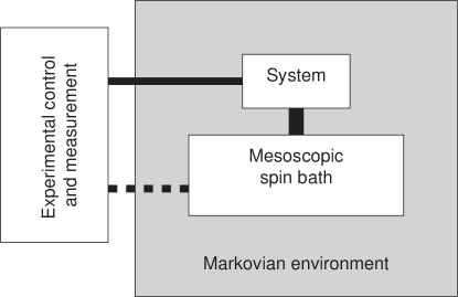
Figure 1: Heirarcichal system–bath–environment coupling. External control of the system (qubit) and measurement are independent of the environment The mesoscopic spin bath is strongly coupled to the system, while the environment provides weak dephasing of the system and spin bath degrees of freedom. Internal dynamics of the spin bath can be ergodic, but some experimental control of the bath may be achieved in limited situations (e.g., through NMR) as indicated.

In many cases, the bias field $\omega$ is large ($|\omega|\gg|\Omega|,|\lambda|$). This is similar to the quantum optical case; accordingly, the standard recipe of transformation into a rotating frame and a rotating wave approximation is also valid here, and off-axis (flip-flop) terms are removed, resulting in a Jaynes-Cummings-like hamiltonian. Roughly speaking, energy cannot be conserved when the system spin flips through changes of the bath state. However, the additional coupling to the bath leads to terms not found in the Jaynes-Cummings hamiltonian.

More explicitly, applying the unitary transformation $U=\exp(-i\omega\hat{S}_{z}t)$, the hamiltonian is

$$\hat{\tilde{H}}_{\rm eff} = \Omega/2[e^{i\nu t}+e^{-i\nu t}][e^{i\omega t}\hat{S}_{+}+e^{-i\omega t}\hat{S}_{-}]+$$ (6)

$$\lambda\hat{S}_{z}\hat{A}_{z}+\lambda/4[e^{i\omega t}\hat{S}_{+}\hat{A}_{-}+e^{-i\omega t}\hat{S}_{-}\hat{A}_{+}]+$$

$$\hat{H}_{A}.$$

When the detuning of the driving field is small, $\delta=(\nu-\omega)\ll\omega$, the highly oscillatory terms in this rotating hamiltonian can be neglected. To do so, the propagator $\hat{U}(t)=\hat{T}\exp(-i\int_{0}^{t}\hat{\tilde{H}}(t^{\prime})dt^{\prime})$ is formally expanded over one period of the applied unitary transformation, $\tau=4\pi/\omega$, and a Magnus expansion Magnus (1954) gives

$$\hat{U}(\tau) = \exp[-i\tau(\sum_{k=0}^{\infty}\hat{H}_{k})]$$ (7)

$$\hat{H}_{0} = 1/\tau\int_{0}^{\tau}\hat{\tilde{H}}(t)~{}dt$$ (8)

$$= \Omega/2[\hat{S}_{+}+\hat{S}_{-}]+(\delta+\lambda\hat{A}_{z})\hat{S}_{z}+\hat{H}_{B}$$

$$\hat{H}_{1} = -i/2\tau\int_{0}^{\tau}\int_{0}^{t_{1}}[\hat{\tilde{H}}(t_{2}),\hat{\tilde{H}}(t_{1})]~{}dt_{2}~{}dt_{1}.$$ (9)

The first term $\hat{H}_{0}$ will be used hereafter. Neglecting $\hat{H}_{1}$ and higher terms of the expansion if formally equivalent to the rotating wave approximation used to derive the Jaynes-Cummings hamiltonian.

II.2 Quasi-static bath assumptions

In standard analyses, usually the bath dynamics are fast relative to the system dynamics, and a Born-Markov approximation is appropriate. However, when the internal bath dynamics are much slower than the system dynamics, the internal bath correlation functions are long lived, and we can consider a quasi-static bath. In this picture, one collective bath operator (here $\hat{A}_{z}$) has, in the Heisenberg picture, a long-lived correlator. In particular,

$$1-\frac{\langle\hat{A}_{z}(t+\tau)\hat{A}_{z}(t)\rangle}{\langle\hat{A}_{z}^{2}\rangle}\ll 1$$ (10)

for $\tau\gtrsim 1/\Omega$. The quasi-static limit is approached when this is satisfied for $\tau>t_{\rm expt}$ (the time for a single experimental run) but not for $\tau\simeq t_{\rm tot}$ (the time to generate enough runs to characterize $\hat{A}_{z}$).

We consider this in detail. Internal dynamics of the spin bath and coupling to the Markovian environment will result in a decay of correlations. A general description of the correlator is

$$\langle\hat{A}_{z}(t)\hat{A}_{z}(t^{\prime})\rangle=\int d\omega\ S(\omega)e^{i\omega(t-t^{\prime})}$$ (11)

where the spectral function $S(\omega)$ has some high frequency cutoff, $\Gamma$, set by the internal dynamics of the bath Cottet and et al. (2001). When $\Gamma\gg\Omega$, the Markovian limit may be reached, and the quasi-static theory developed here is no longer necessary.

When $\Gamma\rightarrow 0$, the thermalization time goes to infinity. Then, while the state of the bath is initially unknown, a series of measurements can be used to estimate the detuning of the system, and thus the value of $\lambda\hat{A}_{z}$ (see, e.g., Refs. Giedke et al., 2005; Klauser et al., 2005). If the manipulation process has a measurement time for a single projection of $\tau_{m}\gtrsim 1/\Omega$, after $n$ such measurements, the error of $\langle\hat{A}_{z}\rangle$ will be

$$\Delta({\langle\hat{A}_{z}\rangle})\simeq\frac{\lambda}{\Omega\sqrt{n}}.$$ (12)

This procedure is exactly that of a classical phase estimation algorithm. It takes a time $\propto n$ to generate a $\sqrt{n}$ improvement in the knowledge of the current value of $\hat{A}_{z}$.

In between lies the quasi-static limit, where a single experiment (i.e., preparation of a given qubit state, evolution under $H_{0}$ for a specified time, followed by projective measurement) can be performed well within the correlation time, but not enough experiments can be performed to well estimate $\hat{A}_{z}$. Qualitatively speaking, this is equivalent to taking a thermal average for the ensemble of measurements, and mathematically the same as the result for the simultaneous measurement of a large number of exactly similar systems. The uncertain knowledge of $\hat{A}_{z}$ leads to dephasing when attempting specific quantum information operations.

As a typical case, consider an internal bath hamiltonian $H_{A}=\hbar\sum_{k}\omega_{B,k}\hat{B}^{k}_{z}$ and a coupling with $\hat{\vec{A}}=\sum_{k}\alpha_{k}\hat{\vec{B}}^{k}$. This could describe nuclear spins for quantum-dot systems, or charge traps. As $[\hat{H}_{A},\hat{A}_{+}]=\sum_{k}\alpha_{k}\omega_{B,k}\hat{B}_{+}^{k}$, the rotating-wave approximation is valid if $\omega_{B,k}\ll\omega$ for all $k$. Then, the application of a large bias field $\omega$, e.g., due to a static magnetic field, makes the interaction essentially static and classical, whereby the system experiences a fluctuating (classical) field $\hat{\vec{A}}$; fluctuations are due to corrections to the rotating wave approximation and coupling to the Markovian environment. Non-classical correlations of the bath, produced by off-resonant interactions Taylor et al. (2005); Klauser et al. (2005) or preparation techniques (e.g. Taylor et al. (2003b)) return the problem to the fully quantum domain.

For example, for electron spin in quantum dots, where the bath is lattice nuclear spins, dipolar diffusion processes lead to flip-flop interactions wherein a spin inside the dot is exchanged with that of a spin outside the dot, producing ergodic dynamics within the bath on ms timescales de Sousa and Das Sarma (2003b); Yao et al. (2005). In contrast, spin-lattice relaxation (coupling to the larger environment) can be minutes to hours in time. Over time, the dipole diffusion destroys the correlations of the $\hat{A}_{z}$ parameter. Detailed calculations, using the method of moments, suggest that diffusion in dots is within an order of magnitude of the bulk diffusion rate Deng and Hu (2005), and this diffusion decorrelates $\hat{A}_{z}$ no faster than the time scale set by the NMR linewidth (10 ms^-1 for GaAs Paget (1982)). Thus the primary effect of spin-lattice relaxation (coupling to a Markovian environment) is to produce an initial thermal state of nuclear spins, while dipole-dipole interactions lead to decorrelation of $\hat{A}_{z}$ (internal bath dynamics).

For concreteness, we choose for our mesoscopic spin bath of $N$ spin-1/2 systems to have the form

$$\hat{A}_{z}=\sum_{k}\alpha_{k}\hat{I}_{z}^{k}$$ (13)

where $\hat{I}_{z}^{k}$ is the spin component corresponding to the $k$th bath spin, and an internal Hamiltonian giving the quasi-static limit. As many bath variables scale as $\sqrt{N\bar{\alpha^{2}}}$, we normalize the $\alpha_{k}$ such that $\bar{\alpha^{2}}=1/N$, thus keeping $\lambda$ as the sole bath strength parameter. The bars above quantities denote statistical averages over static variables. As we have assumed all bath spins are spin-1/2, we can choose the $z$ axis without loss of generality.

II.3 Markovian environment effects

The principle effects of the Markovian environment are two-fold: it leads to relaxation of the qubit system, and it leads to long-time thermalization of the mesoscopic spin bath. We have established that the internal dynamics of the quasi-static bath, combined with coupling to the Markovian environment, will lead to decorrelation of $\hat{A}_{z}$ and dynamic thermalization. For a weakly coupled Markovian environment, with equilibriation times for the bath that are much longer than experimental times, the main effect of the Markovian environment is to produce an initial mesoscopic spin bath state of the form $\rho_{A}\propto e^{-H_{A}/k_{\rm B}T}$.

In general, the additional Markovian environment degrees of freedom will also couple to the system, leading to relaxation and decoherence that we can model with a Lindblad form of the Louivillian of the combined system-spin bath density matrix. Formally, tracing over the environment yields a superoperator (see Eqn. 5)

$${\mathcal{L}}_{\rm env}\rho = 2\gamma_{s}[2\hat{S}_{-}\rho\hat{S}_{+}-\rho\hat{S}_{+}\hat{S}_{-}-\hat{S}_{+}\hat{S}_{-}\rho]$$ (14)

$$+\sum_{k}2\Gamma_{k}\Big{[}2\hat{I}_{-}\rho\hat{I}_{+}-\rho\hat{I}_{+}\hat{I}_{-}-\hat{I}_{+}\hat{I}_{-}\rho$$

$$+2\hat{I}_{+}\rho\hat{I}_{-}-\rho\hat{I}_{-}\hat{I}_{+}-\hat{I}_{-}\hat{I}_{+}\rho\Big{]}$$

corresponding to the Markovian environment. We presume that the spin-bath is in the high temperature limit, while the qubit system only has spontaneous decay. This is consistent with the rotating wave approximation. The resulting equations, with pure radiative decay for the system, are cumbersome to work with, and we will sometimes use the input-output operator formalism, which is formally equivalent by the quantum fluctuation-dissipation theorem.

III Free evolution

In this section, free evolution for a variety of experimentally-relevant situations is considered. Free evolution corresponds to the case of $\Omega=0$, i.e., the absence of driving field. In quantum information, free evolution is equivalent to phase rotations (Z rotations), and the behavior of free evolution is an indicator of how good a quantum memory the chosen qubit provides. The decay of coherence during free evolution due to the mesoscopic spin bath may be severe; however, we consider spin-echo methods as a means of mitigating the bath’s effects.

Equation 8 is the basic Hamiltonian used hereafter; $\hat{A}_{z}$ is given by Eqn. 13. For free evolution, $\Omega=0$, and the Hamiltonian is

$$\hat{H}_{FID}=(\lambda\hat{A}_{z}+\delta)\hat{S}_{z}\ .$$ (15)

For time-dependent $\hat{A}_{z}$ such that $[\hat{A}_{z}(t),\hat{A}_{z}(t^{\prime})]=0$ (appropriate for the specific baths consider in section II), the exact propagator from $t=0$ to time $t$ is

$$U_{FID}(t)=\exp[-i(\delta t+\lambda\int_{0}^{t}\hat{A}_{z}(t^{\prime})dt^{\prime})\hat{S}_{z}]\ .$$ (16)

In the quasi static limit, we may usually replace $\int_{0}^{t}\hat{A}_{z}(t^{\prime})dt^{\prime}$ with $\hat{A}_{z}t$, simplifying evaluation of the propagator.

III.1 Free induction decay

To illustrate free evolution, we start by studying free induction decay (FID), considered for this case by Zurek (1981) and for a dynamical spin bath by Teklemariam et al. (2003). FID corresponds to the decay experienced by a spin coherence (e.g., a density matrix element $|\uparrow\rangle\langle\downarrow|$) during evolution in a Ramsey-type experiment. The system is prepared in the state $|+\rangle=1/\sqrt{2}(|\uparrow\rangle+|\downarrow\rangle)$, with $\langle\hat{S}_{+}(0)\rangle=1/2$, for example, by rotations induced by control of $\Omega$ (considered below). The driving field is turned off ($\Omega=0$) and the system evolves according to the $\hat{S}_{z}$ coupling only. Then,

$$\Phi_{FID}=\frac{\langle\hat{S}_{+}(t)\rangle}{\langle\hat{S}_{+}(0)\rangle}=\left\langle\exp[-i(\lambda\hat{A}_{z}+\delta)t]\right\rangle_{bath}$$ (17)

For an uncorrelated bath ($\langle\hat{I}_{z}^{k}\hat{I}_{z}^{j}\rangle=\langle\hat{I}_{z}^{k}\rangle\langle\hat{I}_{z}^{j}\rangle$ for $k\neq j$) we can write this in terms of individual bath couplingsfoot2

$$\Phi_{FID}=e^{-i\delta t}\prod_{k}\big{[}\cos(\lambda\alpha_{k}t/2)-i\langle 2\hat{I}_{z}^{k}\rangle\sin(\lambda\alpha_{k}t/2)\big{]}.$$ (18)

The minimum of the projection of the actually final state of the desired final state, $F_{FID}=|\Phi_{FID}|^{2}$ is bounded from below by $({\rm Min}_{k}[|\langle 2\hat{I}_{z}^{k}\rangle|])^{N}$. Thus, initial bath polarization for finite $N$ limits the maximum decay.

The initial decay of this coherence is quadratic, giving

$$F_{FID}\simeq 1-\frac{(\lambda t)^{2}}{2}\sum_{k}2\alpha_{k}^{2}(1-\langle 2\hat{I}_{z}^{k}\rangle^{2}),$$ (19)

as shown in the inset of Figure 2. For a large number of spins, the intermediate time decay converges to a Gaussian, $\exp[-(\gamma_{FID}t)^{2}/2]$, with a rate

$$\gamma_{FID}=\lambda\sqrt{\sum_{k}\alpha_{k}^{2}(1-\langle 2\hat{I}_{z}^{k}\rangle^{2})}.$$ (20)

When the inhomogeneity in the $\alpha_{k}$ coefficients is low, the system experiences mesoscopic revival on a time scale given by the single spin coupling strength, $\lambda\bar{\alpha}\simeq\lambda/\sqrt{N}$. This type of revival is shown in Figure 2, where a Gaussian distribution of $\alpha_{k}$ of increasing widths are used, and a bath polarization $P=\langle 2\hat{I}_{z}\rangle=0$ is assumed. These mesoscopic effects for finite spin systems have been investigated in great detail elsewhere Zurek (1981), and we refer readers to those works for a detailed description. In most physical settings, inhomogeneity is large and revival will not be observed. However, for systems where $N$ is small, fluctuations can become substantial even with a large inhomogeneity in the $\alpha_{k}$’s, and such fluctuations have been observed experimentally Teklemariam et al. (2003).

Figure 2: FID evolution ($F_{FID}$) in time scales $\sqrt{N}/\lambda$ for increasing inhomogeneity, $\sigma_{\alpha}=\{0.1,0.3,0.6,1\}/\sqrt{N},N=30,P=0$. The inset shows increasing decay in the short time limit due to increasing inhomogeneity, $\sigma_{\alpha}=\{5,10,20\}/\sqrt{N},N=30,P=0$.

To put the results in an experimental context, we consider a Ramsey fringe experiment. A system is prepared in the $|\downarrow\rangle$ state. A $\pi/2$ pulse is applied along $x$ (denoted $R^{x}_{\pi/2}$), and then at a later time $t$, an opposite, $-\pi/2$ pulse is applied. Afterwards, a projective measurement on $z$ measures the rotation of the $\hat{S}_{y}$ eigenstate due to environmental effects and detuning. In terms of actual experimental implementations, preparation of a spin-down eigenstate and measurement along the $\hat{S}_{z}$ axis is enough, if we use two $\pi/2$-pulses with a delay $t$. Formally, in the limit of perfect pulses the propagator is

$$U_{FID}(t)=R^{x}_{-\pi/2}\exp[-i\lambda\hat{A}_{z}\hat{S}_{z}t]R^{x}_{\pi/2}.$$ (21)

In the limit of perfect pulses, the probability of measuring the final state in the $|\downarrow\rangle$ state is given by $F_{FID}$ as a function of the delay time, $t$. If the system is coupled to a spin bath, it will show Gaussian-type decay in the initial time period. This decay is limited in extent for baths of finite polarization (non-infinite temperature). For a small bath size, mesoscopic fluctations and revival after the initial decay may be evident.

For a series of sequential measurements, the finite correlation time of the bath will be evident. For example, for fixed interaction time $\tau$, a series of measurements $\{M_{k}\}$ giving 1 for $|\downarrow\rangle$ and 0 for $|\uparrow\rangle$ at times $t_{k}$ will manifest correlations due to the correlations of $\hat{A}_{z}$ at the different times, $t_{k}$. Assuming the quasi-static limit, such that $\hat{M}_{k}=\cos^{2}(\lambda\hat{A}_{z}(t_{k})\tau/2)$, we find

$$\langle M_{j}M_{k}\rangle-\langle M\rangle^{2}=\frac{1}{8}\exp[-(\lambda\tau)^{2}\int d\omega S(\omega)(e^{i\omega(t_{j}-t_{k})}-1)]$$ (22)

where the cutoff $\Gamma$ of $S(\omega)$ is such that $\Gamma\tau\ll 1$. Thus, the correlation function for a series of measurements with $\tau\Gamma\ll 1$ in principle allow reconstruction of the spectral function describing $\hat{A}_{z}$. We note that $\gamma_{FID}=\lambda\sqrt{\int S(\omega)d\omega}$.

III.2 Spin-echo decay

As the bath correlation time is long, spin-echo techniques can exactly cancel this type of dephasing. For spin-echo, a $\pi$-pulse is applied in between the two $\pi/2$-pulses; the time delays before and after the $\pi$-pulse are $t_{1}$ and $t_{2}$, respectively. The total evolution is thus

$$U_{SE}(t_{2};t_{1}) = R^{x}_{\pi/2}\exp[-i\lambda\hat{A}_{z}\hat{S}_{z}t_{2}]R^{x}_{\pi}$$ (24)

$$~{}\exp[-i\lambda\hat{A}_{z}\hat{S}_{z}t_{1}]R^{x}_{\pi/2}$$

$$= R^{x}_{-\pi/2}\left(R^{x}_{-\pi}\exp[-i\lambda\hat{A}_{z}\hat{S}_{z}t_{2}]R^{x}_{\pi}\right)$$

$$~{}\exp[-i\lambda\hat{A}_{z}\hat{S}_{z}t_{1}]R^{x}_{\pi/2}$$

$$= R^{x}_{-\pi/2}\exp[-i\lambda\hat{A}_{z}\hat{S}_{z}(t_{1}-t_{2})]R^{x}_{\pi/2},$$ (25)

which is the original FID propagator (Eqn. 21) with $t\rightarrow(t_{1}-t_{2})/2$. The previous results hold but now as a function of the time difference. In particular, no decay occurs when $t_{1}=t_{2}$! The probability of measuring $|\downarrow\rangle$ is

$$F_{SE}(t_{1},t_{2}) = \langle\cos^{2}[\lambda\hat{A}_{z}(t_{1}-t_{2})/2]\rangle$$ (26)

$$= \frac{1}{2}\{1+\exp[-\gamma_{FID}^{2}(t_{1}-t_{2})^{2}/2]\}.$$

Spin-echo fidelity ($F_{SE}(t,t)$) is limited both by the imperfections in the rotations, $R^{x}_{\pi/2}$ and $R^{x}_{\pi}$, Markovian processes that directly lead to decay of $\hat{S}_{z}$, and decay of the correlation function of $\hat{A}_{z}$, i.e., in the interaction picture, $\hat{A}_{z}(t)\neq\hat{A}_{z}(t^{\prime})$ for $t$ much later than $t^{\prime}$. The first type of error, examined in detail below, does not depend on the total time $t_{1}+t_{2}$, while the latter errors do. Neglecting imperfections in rotations, the effect of a correlated bath on spin-echo is a textbook problem, and we merely cite the result here:

$$F_{SE}(t,t) = \frac{1}{2}+\frac{e^{-2\gamma t}}{2}$$

$$\ \ \times\exp[-\lambda^{2}\int S(\omega)\sin^{4}(\omega t/2)/(\omega/2)^{2}d\omega]$$

where we assume $\hat{A}_{z}$ is a Gaussian variable described by the spectral function $S(\omega)$, as per Equation 11. The results of a spin echo experiment allow an alternative method of extracting the correlation function associated with the mesoscopic spin bath. For a spectral function describing the bath with cutoff $\Gamma\ll 1/t$, the echo will decay according to $\exp[-2\gamma t-\lambda^{2}\Gamma^{2}t^{4}/4]$.

For free evolution ($\Omega=0$), used for phase gates and quantum memory, we find that a mesoscopic spin bath leads to dephasing in the quasi-static limit, with a time scale given by $1/\lambda$. Sequential measurements in a Ramsey-type experiment allow for reconstruction of the of the spectral function associated with the bath. Furthermore, spin-echo can be used to reduce the dephasing dramatically.

IV Driven-evolution

While the free evolution of the system is illustrative of quantum memory, a critical operation for quantum information processing is rotations about an axis perpendicular to the applied bias. This is achieved by a pulse in the transverse coupling field strength, $\Omega$, leading to driven oscillations between $|\uparrow\rangle$ and $|\downarrow\rangle$. These Rabi oscillations form the basis for the $x$-axis rotations used, for example, in Ramsey-fringe experiments, and more generally for producing a universal set of single qubit gates.

In practice, the perfect rotations (Rabi pulses) needed to produce perfect rotations are unavailable, due to the finite power available for such pulses. We now consider in detail rotations obtained by driving the system (non-zero $\Omega$ in Eqn. 8) in the presence of the mesoscopic spin bath and Markovian environment. In the Heisenberg picture, the single-spin (system) operator equations of motion are given by

$$\frac{d\hat{\vec{S}}}{dt}=i[H_{0},\hat{\vec{S}}].$$ (28)

For time independent $\hat{A}_{z}$ (quasi-static limit) we can solve these equations exactly, noting that $d/dt~{}\hat{\vec{S}}=\hat{\omega}\vec{n}\times\hat{\vec{S}}$, where

$$\hat{\omega} = \sqrt{(\lambda\hat{A}_{z}+\delta)^{2}+\Omega^{2}};$$ (29)

$$\hat{\vec{n}} = \hat{\omega}^{-1}\left(\begin{array}[]{c}\Omega\\ 0\\ \lambda\hat{A}_{z}+\delta\end{array}\right).$$ (33)

This evolution corresponds to the optical Bloch equations, giving driven rotations of the qubit Bloch vector on the Bloch sphere about an axis $\vec{n}$ at frequency $\hat{\omega}$. The dependence these quantities upon the state of the bath leads to shot-to-shot fluctuations, which broadens ensemble or sequential measurements.

Alternatively, we may write the propagator for $\hat{H}_{0}$ as

$$\hat{U}(t)=\cos(\hat{\omega}t/2)\hat{1}-2i\sin(\hat{\omega}t/2)\hat{\vec{n}}\cdot\hat{\vec{S}}$$ (34)

where we have taken the quasi-static limit, such that $\frac{d}{dt}\hat{A}_{z}\simeq 0$.

Returning to Equations 29–33, we calculate the rotation of an initial $z$ eigenstate with $\langle\hat{S}_{z}(t=0)\rangle=1/2$, i.e., determine the Rabi oscillations expected for the initial state $|\uparrow\rangle$. The field $\Omega$ leads to population and coherence oscillations. Considering the $z$ and $y$ components together, we define

$$\hat{f} = \frac{(\lambda\hat{A}_{z}+\delta)^{2}}{(\lambda\hat{A}_{z}+\delta)^{2}+\Omega^{2}}$$ (35)

$$\hat{\zeta}(t) = \frac{\Omega^{2}\exp(-i\sqrt{(\lambda\hat{A}_{z}+\delta)^{2}+\Omega^{2}}t)}{(\lambda\hat{A}_{z}+\delta)^{2}+\Omega^{2}}.$$ (36)

Then, $\langle 2\hat{S}_{z}(t)\rangle={\rm Re}[\langle\hat{f}+\hat{\zeta}(t)\rangle]$ and $\langle 2\hat{S}_{y}(t)\rangle={\rm Im}[\langle\hat{\zeta}(t)\rangle]$. The value of $\langle\hat{f}\rangle$ is a measure of the maximum contrast of population oscillations, and also gives the steady-state population difference and lineshape; this is approximately maximal for $\delta=-\lambda\langle\hat{A}_{z}\rangle$. $\langle\hat{\zeta}(t)\rangle$ gives the oscillatory part of coherence and population.

IV.1 Steady-state behavior

For long times, the steady state behavior will be given by $\langle\hat{f}\rangle$, which measures the population difference between $\uparrow$ and $\downarrow$. This gives the measureable response of the system to CW excitations of the system. A simple estimate of $\langle\hat{f}\rangle$ is provided by writing $\hat{A}_{z}$ as $\langle\hat{A}_{z}\rangle+\delta\hat{A}_{z}$, and assuming $\langle(a+\hat{A}_{z})^{-2}\rangle=\langle(a+\langle\hat{A}_{z}\rangle)^{2}+\langle\Delta\hat{A}_{z}^{2}\rangle)^{-1}\rangle$. Then,

$$\langle\hat{f}\rangle=\frac{1}{1+\Omega^{2}/[(\delta+\lambda\langle\hat{A}_{z}\rangle)^{2}+\lambda^{2}\langle\Delta\hat{A}_{z}^{2}\rangle]}.$$ (37)

This has a maxima at the mean bath detuning, $\lambda\langle\hat{A}_{z}\rangle$, and as such this point would be the observed zero in detuning. Differences from this observed zero, denoted $\tilde{\delta}$, gives an absorption spectrum of

$$\langle\hat{f}\rangle=1-\frac{\Omega^{2}}{\tilde{\delta}^{2}+\lambda^{2}\langle\Delta\hat{A}_{z}^{2}\rangle+\Omega^{2}}$$ (38)

which behaves as a Lorenztian with a linewidth given by the combined power broadening and bath broadening for $\Omega\ll\lambda\langle\Delta\hat{A}_{z}^{2}\rangle^{1/2}$.

The approximations used for this simple estimate break down for large bath strength. To find this behavior in the strong bath limit, where higher order moments are important, we need not assume that the bath density matrix is uncorrelated, as before, but rather that the bath density matrix is diagonal in an eigenbasis of the bath operator, $\hat{A}_{z}$. foot3 This would be appropriate for nuclei interacting with an electron spin in a quantum dot at finite magnetic field, or for charge traps capacitively coupled to the system.

We can evaluate $\langle\hat{f}\rangle$ by tracing over the bath density matrix, replacing $\rho_{bath}=\sum_{\lambda A_{z}}\rho_{\lambda A_{z}}|\lambda A_{z}\rangle\!\langle\lambda A_{z}|$ with $\rho(\Lambda)$. The integrals involved are solved in Appendix A. We note that the result is

$$\langle\hat{f}\rangle\simeq 1-\rho(-\delta)\sqrt{2\pi\Omega/u}$$ (39)

for the lineshape. This has assumed that $u^{-1}$ is a frequency scale over which the bath density of states is relatively flat, and as such can be Taylor expanded to second order. This time scale is

$$u=\frac{5}{4\Omega}-\frac{\Omega\rho^{\prime\prime}(-\delta)}{\rho(-\delta)}.$$ (40)

In other words, driven oscillations can measure the bath density of states as a function of detuning, convolved with a kernel of width $u^{-1}$. We plot several lineshapes in Fig. 3.

Essentially, we find that the steady-state behavior of the system indicates a maximum of population in the state opposite the initial state at a detuning $\delta=-\lambda\langle\hat{A}_{z}\rangle$. In addition, in the weak field limit, the line shape provides a sensitive measure of diagonal components of the bath’s density matrix, so long as a calibration of $\Omega$ independent of the bath exists.

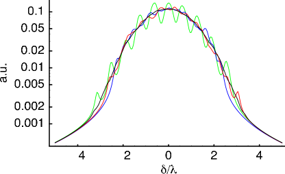
Figure 3: Lineshapes for a bath with $N=10$ and increasing inhomogeneity [$\sigma_{\alpha}$ = 0.1(green),0.5(red),1(blue)]. The additional line is $N=20,\sigma_{\alpha}=0.5$ (black).

IV.2 Time-dependent behavior

We now consider the actual, observable population and coherence oscillations induced by a driving (Rabi) field. Looking at the explicit time dependence, we consider the envelope of oscillations given by $|\hat{\zeta}(t)|$. The initial decay is quadratic, $(1-\langle f\rangle)[1-(\gamma_{\Omega,0}t)^{2}/2]$, and when renormalized to give maximal contrast, it has a width

$$\gamma_{\Omega,0} = \sqrt{-\frac{d^{2}}{dt^{2}}\Big{|}\frac{\langle\hat{\zeta}(t)\rangle}{(1-\langle\hat{f}\rangle)}\Big{|}_{t=0}}$$ (41)

$$= \frac{\Omega^{2}}{1-\langle\hat{f}\rangle}\times$$

$$\sqrt{\left\langle\frac{1}{(\lambda\hat{A}_{z}+\delta)^{2}+\Omega^{2}}\right\rangle-\left\langle\frac{1}{\sqrt{(\lambda\hat{A}_{z}+\delta)^{2}+\Omega^{2}}}\right\rangle^{2}}.$$

This suggests that measurements of such short time decay will measure second order moments of the bath operators.

While the short time behavior is consistent with Gaussian decay, as would be expected from a non-Markovian, non-dissipative bath, the long time behavior is a power law.

The integrals involved are solved in Appendix A; essentially we solve for $\langle\hat{\zeta}(t)\rangle$, and find

$$\langle\zeta(t)\rangle\approx\rho(-\delta)e^{-i\Omega t}\frac{\sqrt{2\pi\Omega}e^{-i\theta(t)}}{\sqrt{\tau(t)}}.$$ (43)

where the time scale for phase shift, and phase shift angle, are given by

$$\tau(t) = \sqrt{t^{2}+u^{2}}$$ (44)

$$\theta(t) = 1/2\tan^{-1}\left[t/u\right],$$ (45)

and $u$ is the same as Eqn. 40.

We note that this result is much more robust than Eqn. 39, due to the oscillatory terms in the integrand canceling out behavior in the exponential tail. This solution encompasses the long time behavior ($t\gg\Omega^{-1}$), and breaks down if $\rho_{sym}$ is singular for $\omega\geq\Omega$ or if $u<0$ foot4 . The lack of dependence of the effective Rabi frequency on the detuning follows naturally from situations where the density of states at $-\delta$, $\rho(-\delta)$ is sizeable: that portion of the density of states is resonant, and the resonant behavior dominates. When $u<0$, we may be in the detuning dominated regime, and these results no longer hold.

IV.3 Discussion

The long-time behavior, Eqn. 43, may seem peculiar at first. The power-law decay envelope comes from the portion of the bath density of states that is “on-resonance” with the oscillations. In particular, for short times, Rabi oscillations are insensitive to detunings less than the Rabi frequency. This window narrows for longer time, leading to the observed power law behavior. More curiously, for times $t\gg u$, there is an overall phase shift of $\pi/4$ that is independent of many of the parameters of the bath. This dynamic shift eludes a similar immediate qualitative description, arising from the continuity of the bath density of states and the pole induced by probing of the bath (by means of the applied Rabi field) that is insensitive to first derivatives of the bath, i.e., bath variables come in only in their quadrature and higher moments.

It is crucial to distinguish these results from more standard inhomogeneous broadening results. Unlike the case of Doppler broadening, for example, in this system the individual system detunings do not change as a function of time. When the correlation function is short-lived, the behavior would instead follow directly from the well understood results describing inhomogenous broadening due to Doppler shifts of laser-induced Rabi oscillations.To extend these results to describing inhomogeneous broadening in ensembles of self-assembled quantum dots, for example, would require considering the additional effect of inhomogeneity in the Rabi strength, $\Omega$, and it is unclear that the corresponding phase shift would behave in a similar manner to the case of a single Rabi frequency. As such, that analysis is beyond the scope of this paper.

To compare these analytical results to exact solutions, we solve the system for finite spin, where we exactly evaluate the trace for finite $N$. In the homogeneous case, the Dicke picture of collective angular momentum allows us to go to large $N$, while the inhomogeneous case requires exponential operations for the exact value, but can be simulated through stochastic modeling of the trace function. We compare several different values of inhomogeneity and bath size $N$ in Figure 4, and show strong quantitative agreement between the short time and long time approximations with the numerical evolution. We also show the convergence to full contrast for a fixed time and varying Rabi power.

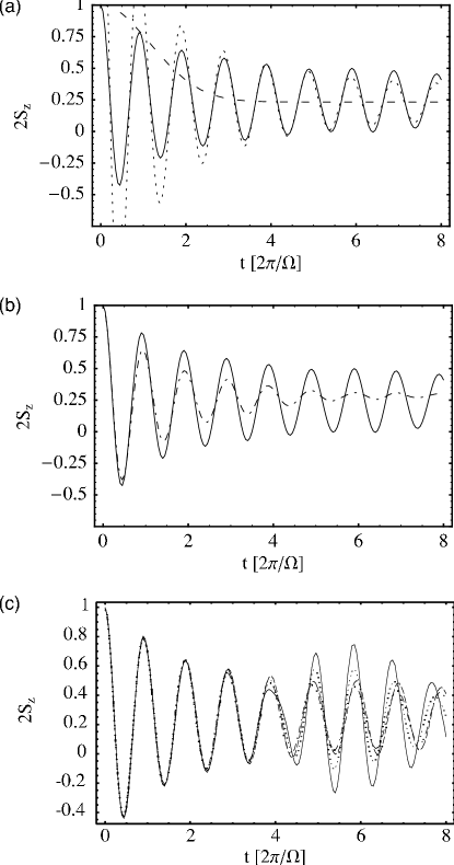
Figure 4: (a) Comparison of short time and long time theoretical results to analytic results, with $\sigma_{\alpha}=\bar{\alpha}/2$, $\lambda=1$, $N=20$, and $\Omega=2\pi$. The exact solution (solid line) compares well with the short time decay (dashed line) and the long time tail plus phase shift (dotted line). (b) Comparison of the same exact result with the case with $\gamma=0.5$ (dotted line). (c) Fluctuations for $N=$6 (solid),10 (dashed), 14 (dashed-dotted), and 20 (dotted).

The previous analysis assumed that the bath density of states could be taken as a Gaussian, which can be shown to reduce to the assumption of Gaussian noise Gardiner (1985). However, inclusion of non-Gaussian effects leads in the general cases to integrals without easy solution.

The deviation from Gaussian noise for the fourth order at $T=\infty$ is

$$\frac{\langle\hat{A}_{z}^{4}\rangle-3\langle\hat{A}_{z}^{2}\rangle^{2}}{3\langle\hat{A}_{z}^{2}\rangle^{2}}\simeq-2/N.$$ (46)

To investigate the role non-Gaussian effects play, simulations with finite numbers of spin were conducted; the thermodynamic limit recovers Gaussian statistics. For small inhomogeneity, Fig. 4c indicates that increasing spin number decreases the amplitude of fluctuations from the expected Rabi signal. Increasing inhomogeneity leads to an apparent additional reduction of fluctuations, though quantifying this effect remains difficult.

IV.4 Inclusion of the Markovian environment

For completeness, we now add the coupling of the qubit to an additional, Markovian environment, with a corresponding “radiative” decay to the ground state with a rate $\gamma$. The optical Bloch equations must now be modified to include this decay, and exact solutions, while available, are cumbersome. However, the case of FID, with $\Omega=0$, is immediately understandable. In the Heisenberg picture, we write

$$\frac{d\hat{S}_{+}}{dt}=-\gamma\hat{S}_{+}+i\lambda\hat{A}_{z}\hat{S}_{+}+\hat{\mathcal{F}}_{+},$$ (47)

where the stochastic input field $\hat{\mathcal{F}}_{+}$ has the standard Markovian kernel, $\langle\hat{\mathcal{F}}_{-}(t)\hat{\mathcal{F}}_{+}(t^{\prime})\rangle=2\gamma\delta(t-t^{\prime})$. Solving this equation of motion exactly for $\langle\hat{S}_{+}(t=0)\rangle=1/2$ gives

$$\Phi_{FID,\gamma}=\frac{\langle\hat{S}_{+}(t)\rangle}{\langle\hat{S}_{+}(0)\rangle}=\left\langle\exp(-i\lambda\hat{A}_{z}t-\gamma t)\right\rangle_{bath}=\Phi_{FID}e^{-\gamma t}.$$ (48)

The Markovian environment results in irreversible exponential decay, which would be unaffected by any spin-echo experiment. For long correlation time baths, spin-echo experiments provide a direct measure of the Markovian component of the decay.

For the case with $\Omega\neq 0$, we use the analytical evolution for solving the Kraus operator form for the Bloch vector, $d\hat{\vec{S}}/dt=M\hat{\vec{S}}+\vec{u}$ and evaluating the expectation values of all functions of $\hat{A}_{z}$ at each time point. The results are cumbersome, and checked only numerically. Qualitatively comparing the result, shown in Figure 4b, to the $\gamma=0$ case, we see that the crucial features of phase shift and fast initial damping with long-lived oscillations remain, but that the steady state population difference is shifted, and the oscillations are eventually damped by the exponential tail. The corresponding lineshape is approximately

$$\langle\hat{f}\rangle=1-\left\langle\frac{\Omega\gamma}{[(\gamma/2)^{2}+(\lambda\hat{A}_{z}+\delta)^{2}+\Omega^{2}]}\right\rangle$$ (49)

Finally, we now consider the effect decorrelation of $\hat{A}_{z}$ plays in the observed oscillations. Unlike the case of free evolution, $[H_{0}(t),H_{0}(t^{\prime})]\neq 0$, leading to difficulties in analytical evaluation of the propagator including decorrelation effects. We can, however, consider it partially by use of a Magnus expansion, in the limit of weak to intermediate strength mesoscopic spin bath.

Formally, we transform $H_{0}$ to the interaction picture with respect to $\Omega\hat{S}_{x}$, and with $\delta=0$, giving

$$\tilde{H}=\lambda\hat{A}_{z}[\cos(\Omega t)\hat{S}_{z}+\sin(\Omega t)\hat{S}_{y}]$$ (50)

If we assume $\hat{A}_{z}$ varies on time scales much longer than $1/\Omega$, we can use a magnus expansion. The expansion of this Hamiltonian at peaks in the expected oscillations ($\tau=2\pi/\Omega$) yeilds

$$U_{eff}(\tau)=\exp[-i\tau(H_{0}+H_{1}+\ldots)]$$ (51)

with

$$H_{0}=0$$ (52)

$$H_{1}=2(\lambda\hat{A}_{z})^{2}/\Omega\hat{S}_{y}\ .$$ (53)

We neglect higher order contributions by assuming that $\langle\hat{A}_{z}^{2}\rangle^{4}\lambda^{4}/\Omega^{4}\ll 1$. Thus, the envelope of oscillations should be determined by

$$U_{eff}(t)=\exp[-i\int_{0}^{t}\frac{2(\lambda\hat{A}_{z}(t^{\prime}))^{2}}{\Omega}dt^{\prime}\hat{S}_{y}]\ .$$ (54)

where we have assumed that over a time $\tau$, $\hat{A}_{z}(t)$ is fixed. We note that this form of quadratic noise has been investigated in detail Makhlin and Shnirman (2004). The lowest order perturbative expansion requires determining the spectral function

$$S_{A^{2}}(\omega)=\int\frac{d\tau}{2\pi}\langle\hat{A}_{z}(t+\tau)^{2}\hat{A}_{z}(t)^{2}\rangle e^{-i\omega\tau}\ .$$ (55)

Assuming Gaussian statistics for $\hat{A}_{z}$, we find

$$\langle Az(t)^{2}\hat{A}_{z}(t^{\prime})^{2}\rangle=(\int d\omega S(\omega))^{2}+2(\int d\omega S(\omega)e^{i\omega(t-t^{\prime})})^{2}$$ (56)

The resulting decay of oscillations should be given by

$$\exp(-\frac{4\lambda^{4}}{\Omega^{2}}\int d\omega S_{A^{2}}(\omega)\frac{\sin^{2}(\omega t/2)}{(\omega/2)^{2}})$$ (57)

Oscillations with low frequency noise for $S(\Omega)$ are shown in Fig. 5.

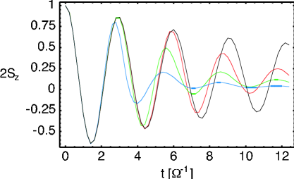
Figure 5: Expected value of $2\hat{S}_{z}$ as a function of time for an initial state $\hat{S}_{z}=1/2$, with driving and low frequency noise $\lambda=\Omega/2$. Decorrelation rates of 0 (black), $\Omega/100$ (red), $\Omega/30$ (green) and $\Omega/10$ (blue) are shown. It is apparent that decorrelation leads to steady state values of zero, faster than $1/\sqrt{t}$ decay, and reduced phase shift (from $\pi/4$).

We remark that for time independent $\hat{A}_{z}$ and a Gaussian density of states we can evaluate the expected envelope of oscillations,

$$\langle U_{eff}(t)\rangle=(1+2it\rho^{\prime\prime}(0)/\rho(0)\Omega)^{-1/2}\ ,$$ (58)

reproducing the $1/\sqrt{t}$ long-time tail found by more exact means. Furthermore, as $\langle\hat{A}_{z}^{2}\rangle\neq 0$ in general, a phase shift due to small rotations around $\hat{S}_{y}$ after each Rabi oscillation should be expected.

V Application to experimental systems

We now consider the physical systems where the quasi-static bath assumptions are valid. One case is nuclear spins interacting with an electron spin in a quantum dot. There, the dominant internal bath Hamiltonian is aligned with the bath-interaction, and $[\hat{H}_{B},\hat{A}_{z}]=0$ identically Taylor et al. (2003a); Mehring (1976). Another system is superconducting qubits, where charge-traps and other few-state fluctuators play a similar role. Finally, some NMR systems with one probed spin (e.g., a Carbon-13) is coupled to many spins (e.g., nearby hydrogens).

V.1 Electron spin in quantum dots

The hyperfine interaction between the electron and the nuclear spins is given by

$$H_{QD}=\gamma_{e}B_{0}\hat{S}_{z}+\lambda_{QD}\sum_{k}\alpha_{k}\hat{\vec{S}}\cdot\hat{\vec{I}}+\gamma_{n}B_{0}\sum_{k}\hat{I}_{z}^{k}$$ (59)

where the $\alpha_{k}\propto|\psi(r_{k})|^{2}$ are weighted by the electron wavefunction’s overlap with lattice site $k$. For GaAs quantum dots with $N$ nuclear spins, $\lambda_{QD}\simeq 207{\rm ns}^{-1}/\sqrt{N}$ Paget et al. (1977), with the normalization condition $\sum_{k}\alpha_{k}^{2}=1$. Identifying $\gamma_{e}B_{0}=\omega$ and adding a time dependent ESR field in the $x$-axis the model Hamiltonian is recovered, with $\lambda=\lambda_{QD}$. In the case of a large applied magnetic field ($\omega\gg\lambda_{QD}$), the results heretofore derived hold.

While experiments investigating ESR and spin dephasing in single quantum dots are ongoing, the contraints imposed by the quasi-static limit make standard ESR technically difficult to achieve. For small quantum dots (e.g. single electron quantum dots), $\lambda_{QD}\gtrsim 0.1$ ns^-1 ($N\simeq 10^{5}$). If the decorrelation rate $\Gamma$ is determined by dipolar-diffusion processes, it can be no faster than 10 ms^-1, the linewidth of NMR in bulk GaAs, and the quasi-static limit is appropriate. For the quasi-static field to be overcome, either many measurements must be taken in the correlation time of the bath, or ESR field’s Rabi frequency $\Omega$ must be much larger than $0.1$ ns^-1. This latter requirement may be quite difficult for current experimental parameters. Active correction sequences may lower this rate, by averaging through NMR pulses the dipolar interaction Waugh et al. (1968); Mehring (1976), making it possible to perform accurate phase estimation within the enhanced correlation time of the bath.

There is another important situation where the mesoscopic bath picture holds: during an exchange gate Loss and DiVincenzo (1998); Petta et al. (2005). In particular, for two tunnel coupled quantum dots, each in the single-electron regime, the overall Hamiltonian is

$$H_{DQD}=H_{QD}^{1}+H_{QD}^{2}+J\hat{\vec{S}}^{1}\cdot\hat{\vec{S}}^{2}$$ (60)

where $J$ is the exchange interaction between the two dots. While the $m_{s}=\pm 1$ triplet states ($|\uparrow\uparrow\rangle,|\downarrow\downarrow\rangle$) are well separated by Zeeman energy, the $m_{s}=0$ states ($|\uparrow\downarrow\rangle,|\downarrow\uparrow\rangle$) are nearly degenerate. In the basis $\{|\uparrow\downarrow\rangle,|\downarrow\uparrow\rangle\}$, this two-level system is described by the Hamiltonian

$$H_{m_{s}=0}=\left(\begin{array}[]{cc}-\lambda\hat{A}_{z}^{(DQD)}/2&\Omega/2\\ \Omega/2&\lambda\hat{A}_{z}^{(DQD)}/2\end{array}\right)$$ (61)

where $\lambda\hat{A}_{z}^{(DQD)}=\sum_{k,i=1,2}\lambda_{QD}^{i}(-)^{i}\alpha_{k}^{i}\hat{I}_{z}^{k,i}$ is the bath parameter for this two-level system, and $\Omega=J$. This Hamiltonian maps exactly to Equation 8.

Recently experiments demonstrated coherent oscillations driven by controlled exchange interactions Petta et al. (2005). The system was prepared in an eigenstate of the mesoscopic spin bath interaction (e.g., the $|\uparrow\downarrow\rangle$ state) and coherent oscillations between $|\uparrow\downarrow\rangle$ and $|\downarrow\uparrow\rangle$ were driven by applying a pulse of non-zero $\Omega$ for finite time. These experiments correspond exactly to the driven evolution examined in the previous section. As such, for small exchange values ($\Omega\simeq\lambda$) we expect the exchange operations to exhibit the characteristic power-law decay and phase shift found in this work. Our approach agrees with system-specific theoretical predictions of Ref. Coish and Loss, 2005.

V.2 Superconducting qubits

The quasi-static assumptions also hold for bistable two-level fluctuators, where the $\hat{I}_{z}$ eigenvalues denote which state is populated, and the dominant interaction with a charge system is a conditional capacitive energy, leading to a $\hat{S}_{z}\hat{I}_{z}$ interaction between the two. Furthermore, $1/f$-type two-level fluctuators, considered the source of most Josephson junction dephasing Kautz and Martinis (1990); Galperin and Gurevich (1991), are quasi-static in the high frequency regime, i.e., above the bath cutoff. Curiously, the spin-boson model Caldeira and Leggett (1983) does not fulfill this criterion. Other pseudo-spin systems, such as flux qubits, may or may not have this structure, depending on the bath degrees of freedom.

The extension of our results to superconducting qubit experiments is motivated by results characterized by low contrast, long-lived Rabi oscillations, similar to those exhibited in our model. For a system with some minimum time of applied Rabi field (as is often the case in these experiments) the initial, fast decay could be encompassed by oscillations occurring within this minimum time, while the observable oscillations correspond to the long-time tail.

Of the superconducting qubit experiments, we focus on Ref. Martinis et al., 2002, as 1/f noise is a dominant term for similar devices in CW behavior. In addition, there are observed resonances with flucuators in the measurement spectrum Simmonds et al. (2004), which suggests that coherent coupling to these two-level systems may be possible. A model which includes preparation and measurement errors is considered in Appendix B; we note the results here. We find that in the low power regime, our model explains the observed behavior, but at higher powers incoherent heating due to driving microwaves play an important role as well.

Fitting the parameters from Appendix B to the Rabi oscillations shown in Ref. Martinis et al. (2002) yield the values in Table 1. The results are consistent with bath domination for low power ($\Omega<0.5{\rm ns}^{-1}$) and heating / preparation error dominating at high power. This gives the characteristic low contrast oscillations observed, even though the static measurement efficiency is quite high (order 75-85%). The resulting oscillations are compared to Ref. Martinis et al., 2002 in Fig. 6.

Table 1: Fitted values (explained in Appendix B) for the model describing the experiments of Ref. Martinis et al., 2002. The values in parantesis are the 90% confidence intervals of the fit.

$M_{\uparrow\uparrow}$	0.75(4)
$M_{\downarrow\downarrow}$	1.00(3)
$\Gamma$	0.10(4) ns-1
$\lambda$	0.27(1) ns-1

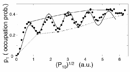
Figure 6: Plot of oscillations reproduced from Ref. Martinis et al., 2002 (filled circles). The probability of spin flip, $P_{1}=\frac{1}{2}-\langle\hat{S}_{z}(t)\rangle$ is plotted versus Rabi frequency $\Omega\propto P_{10}^{1/2}$ a fixed Rabi evolution time of 25 ns. Overlaid for the given fit parameters are the expected values from our model (solid line).

V.3 Other systems

Under certain conditions, NMR systems may be described by a quasi-static mesoscopic spin bath . For example, large molecules or crystalline structures with long correlation times and coherent dynamics within the molecule, where one or few spins are coupled to many adjacent spins in a static configuration, may be described by our model. In contrast, liquid state NMR with small molecules has bath characteristics dominated by transient couplings to other molecules, and our model is inappropriate.

One example is in cross-polarization experiments on solid-state ferrocene, where defocusing sequences are applied to generate a Hamiltonian equivalent to Eqn. 8 Chattah et al. (2003). By direct observation of the cross-polarization signal, driven evolution may be observed. We remark that previous experiments, investigating spin-bath coupling in free evolution Teklemariam et al. (2003) will not show this behavior. System specific work Danieli et al. (2005) is in general agreement with our results.

VI Methods to mitigate bath effects

While the strongly coupled mesoscopic spin bath leads to dephasing during free evolution and reduced contrast and a dynamical phase shift during driven evolution, the long-time correlation of the bath allows for correction. We start by considering spin-echo-type passive error correction, which can be implemented if a sufficiently strong Rabi frequency for driving is available. We then consider how entropy transfer from the quasi-static bath to the environment (bath-cooling) may be an effective alternative means of reducing the damping due to the bath. In essence, for specific bath models, it may be possible to prepare coherences in the bath which effectively reduce the uncertainties engendered by the bath. The inherently quantum mechanical nature of this leads us to consider this mechanism as environmental squeezing.

VI.1 Passive error correction

With strong Rabi power ($\Omega\gg\lambda$), high fidelity Rabi oscillations are possible even in the presence of the mesoscopic spin bath. This is the power-broadened limit. The error of such pulses scales as $(\lambda/\Omega)^{2}$ and as such determining the quasi-static bath strength for a given system will yield the required Rabi power to overcome the effects of the bath through passive error correction.

In this limit, spin-echo techniques work well to greatly extend the lifetime of oscillations, and passive error correction Zanardi and Rasetti (1997) will be straightforward to implement. Higher order pulse sequences than those considered in Section III may lead to further improvement Facchi et al. (2005). Other techniques, such as quantum bang-bang Viola and Lloyd (1998), are already implicit in this analysis in the form of coherent averaging theory Mehring (1976).

VI.2 Cooling the bath

When experimental limitations of Rabi power or other experimental difficulties make minimization of the coupling strength impossible, the quasi-static bath remains a problem uncorrectable by passive error correction. Then, active cooling techniques may be a useful alternative. We now outline how, for the specific case of scalar interactions with the bath, qubit manipulation may lead to efficient entropy transfer from the mesoscopic spin bath to the qubit system. By exploiting resonances between the bath and system, we may cool the bath degrees of freedom. Furthermore, in the quasi-static limit, coherences developed between bath spins can lead to additional improvements through a form of squeezing.

To illustrate cooling, the explicit case of an electron spin in a quantum dot is illuminating. For that system, the full spin-coupling (including the terms previously neglected in the rotating wave approximation) is a scalar interaction Taylor et al. (2003a),

$$\lambda\hat{\vec{S}}\cdot\hat{\vec{A}}=\lambda\hat{\vec{S}}\cdot\left(\sum_{k}\alpha_{k}\hat{\vec{I}}^{k}\right).$$ (62)

The dominant terms in the internal Hamiltonian of the nuclear spins is

$$H_{A}=\sum_{k}\omega_{k}\hat{I}_{z}^{k}\ ,$$ (63)

due to the Larmor precession of the nuclear spins in the external magnetic field. When the effective splitting of the qubit (electron spin) is comparable to $\omega_{k}$, the electron spin comes into resonance with the nuclear spins. In essence, by tuning the system near such a “noise-resonance”, the bath can be driven in a double-resonance manner (analogous to electron-nuclear double resonance, ENDOR), where the on-axis ($z-z$) coupling is offset by the changing frequency of the applied Rabi field. Before, the internal spin dynamics were considered to be much slower, i.e., $\omega_{k}\ll|\omega+\lambda\langle\hat{A}_{z}\rangle|$. For double-resonance, this condition is no longer satisfied, and the quasi-static approximations begin to break down.

For this resonant regime, the reader is referred to previous work on electron spin cooling Imamolgu et al. (2003); Taylor et al. (2003b) for the details of the process. The benefits of cooling are outlined here. In the fully cooled state, the quasi-static bath acts entirely as an additional detuning on the system, as $\langle\hat{A}_{z}\rangle^{2}=\langle\hat{A}_{z}^{2}\rangle$. Near such high polarization, the quasi-static bath effects do not supress Rabi and Ramsey-type effects, as the bath strength parameter at high temperature ($\lambda\sqrt{\langle\hat{A}_{z}^{2}\rangle}$) is greatly reduced at low temperature. Quantitatively, this improvement is given by the ratio of $\gamma_{FID}$ (Eqn. 20) at high and low polarizations, which is $\eta=\sqrt{1/(1-P)}$ for a polarization $P$ of the bath (neglecting inhomogeneous corrections). In terms of experimental observables, it should result in an increase in the observed contrast of Rabi oscillations and improved Ramsey signals as if the bath strength parameter, $\lambda$, had been reduce by the improvement factor $\eta$. The improvements will be limited by coherences developed within the bath, by the correlation time of the quasi-static bath, which will limit the lifetime of the cooling, and by other, non-local (and correspondingly difficult to cool) degrees of freedom, implicit in the Markovian environment component of this model.

Cooling could proceed along the following lines. The system is prepared in a $|\downarrow\rangle$ state by coupling to the Markovian environment, e.g., by moving to a strongly coupled region of parameter space. This is the current preparation method for superconductor-based qubit designs; in quantum dots, the energy difference between spin states due to zeeman splitting or exchange interactions allows preparation by controlled coupling to a nearby Fermi sea Petta et al. (2005). Then a weak, negatively detuned Rabi field is applied for a short time (order one Rabi flop). This process is repeated many times. Including state measurement after the Rabi field will allow measurement of the cooling efficiency, as the bath will lead to additional flip to the $|\uparrow\rangle$ state in the far detuned regime. In some cases, where the natural frequencies of the bath degrees of freedom are large, resonances between the bath and system may be observed. Tuning to the “red” side of these resonances will also force cooling to occur.

As cooling is effected only through the logical basis states (the qubit states of up and down), it is not necessarily efficient. For a simple scalar coupling (e.g. a hyperfine interaction), cooling proceeds due to the action of the $\hat{A}_{-}$ operator, where

$$\hat{A}_{-}=\sum_{k}\alpha_{k}\hat{I}_{-}^{k}$$ (64)

However, states $|\mathcal{D}\rangle$ with the property $\hat{A}_{-}|\mathcal{D}\rangle=0$ cannot cool under this action. This is similar in practice to single mode cooling, and as such it does not greatly improve the bath polarization or entropy Taylor et al. (2003b) for intermediate or larger bath sizes. However, these states do have a useful symmetry property, namely they are “dark” under the action of the collective lowering operator. Thus, the natural state of the density matrix after many cycles of cooling is

$$\hat{\rho}=\sum_{\beta}\rho(\beta)|{\mathcal{D}}(\beta)\rangle$$ (65)

where the sum is over other degeneracies (see Arecchi et al. (1972); Taylor et al. (2003b) for details). We now indicate how cooling limited to polarizations such that $\eta$ remains order unity can still be sufficient to greatly reduce the dephasing induced by the mesoscopic spin bath.

In particular, if this cooling can be applied along the axis of Rabi oscillations (rather than the $z$ axis), the effects of such marginal cooling are immediately apparent. In particular, the component of noise in the $x$ and $y$ axes are averaged by the bias, $\omega$, while the $z$ axis is only averaged by the driving field, $\Omega$. If the $z$ component of the bath noise can be reduced, the corresponding Rabi and Ramsey signals will be improved. In the case of homogeneous coupling ($\alpha_{k}=1/\sqrt{N}$) to the environment, it can be shown immediately that cooling into dark states decreases the quadrature in the non-cooled axes, i.e.,

$$\langle\hat{A}_{z}^{2}\rangle=1/\sqrt{N}$$ (66)

which is a $\sqrt{N}$ improvement over the uncooled state. As the other quadratures correspond to noise suppressed by the bias, the effect on experiment is immediate and possible quite useful. Such Rabi-axis cooling can be achieved for nuclei in quantum dots by first cooling along the natural ($z$) axis, followed by a NMR $\pi/2$-pulse to rotate the nuclear coherences to be parallel to the driving field.

The coherences between spins in the bath have a limited lifetime, determined by the decay of the correlation functions of the bath. Therefore, for this process to be useful, the qubit-bath interaction must be much faster than the bath decorrelation time, but this is exactly the quasi-static approximation already made. Before each run of a Rabi oscillation-type experiment, a cooling sequence could be applied, to keep the bath degrees of freedom. The resulting oscillations should reflect the “cooled” bath results, and as such could provide a substantial improvement over uncooled systems.

VII Conclusions

The response of a two-level system (a qubit) with driving fields coupled to a local, mesoscopic collection of finite-level systems and with additional coupling to a larger, Markovian environment has analyzed in this paper. The natural simplifications of the Hamiltonian lead to a quasi-static regime, wherein bath correlation functions are long-lived when compared to experimental manipulation and measurement time scales. However, decorrelation of the bath and dynamic thermalization processes lead to apparent decay when a single-qubit is manipulated and measured repeatedly. The large variations of bias produced by the quasi-static bath can be difficult to correct with limited Rabi frequency ranges accessible to experiments.

The simple case of free induction decay demonstrates the role increasing bath strength and non-Markovian effects have to play on the short term, non-exponential decay, while finite number effects can lead to revivals and fluctuations, distinctly mesoscopic effects. This illustrates explicitly the non-Gaussian nature of the bath.

In the presence of weak fields, a line-shape distinctive to the spin-bath model is discovered, though inclusion of additional (Markovian) decoherence and dephasing recovers the expected Lorentzian behavior. As the driving field’s strength is increased, Rabi oscillations are possible, but for short times there may be a phase shift of order $\pi/4$ and fast initial decay of the oscillation envelope. However, longer times, with only a power law decay going as $t^{-1/2}$, will most likely be dominated by other, exponential decay processes. As a result, a quasi-static bath could lead to reduced contrast of oscillations that may be consistent with experimental observations of superconducting qubit devices. In addition, experiments with single- and double-quantum dots may probe this quasi-static bath model more directly.

Finally, the role of passive error correction, quantum bang-bang, and environment cooling have been considered, with each appropriate for different ranges of parameters. It may be that as the understanding of quasi-static, local baths increases the means to mitigate their effect will become more apparent. This is a first and crucial step towards that end.

The authors would like to thank A. Imamoglu, D. Loss, J. M. Martinis, H. Pastawski, A. Sorensen, and C. van der Wal for helpful discussions. This work has been supported in part by NSF and ARO.

Appendix A Integrals involved in driven evolution

We now solve the integrals necessary to evaluate $\langle\hat{f}\rangle$ and $\langle\hat{\zeta}(t)\rangle$ for a given bath density matrix, $\rho_{bath}$. Taking the continuum limit for this density matrix, we can evaluate a function $h(\lambda\hat{A}_{z})$ as

$${\rm Tr}[h(\lambda\hat{A}_{z})\hat{\rho}_{bath}] = \sum_{\Lambda}h(\Lambda)\rho_{\Lambda}$$ (67)

$$\rightarrow \int_{-\infty}^{\infty}d\Lambda h(\Lambda)\rho(\Lambda)$$ (68)

Accordingly, the long time population difference, given by $\langle\hat{f}\rangle$ has the form

$$\langle\hat{f}\rangle=1-\sum_{\Lambda}\rho_{\Lambda}\langle\Lambda|\frac{1}{1+(\frac{\delta+\lambda\hat{A}_{z}}{\Omega})^{2}}|\Lambda\rangle$$ (69)

where $\Lambda$ is the eigenvalue of $\lambda\hat{A}_{z}$. Going to the continuum limit, and assuming the power is weak (appropriate for lineshape measurements),

$$\langle\hat{f}\rangle=1-\int_{-\infty}^{\infty}d\Lambda~{}\rho(\Lambda)\frac{\Omega^{2}}{(\Lambda+\delta)^{2}+\Omega^{2}}$$ (70)

Furthermore, the integral depends only upon $\tilde{\omega}=\sqrt{(\Lambda+\delta)^{2}+\Omega^{2}}$, so we define the symmetric density,

$$\rho_{sym}(\omega)=\rho(-\delta-\sqrt{\omega^{2}-\Omega^{2}})+\rho(-\delta+\sqrt{\omega^{2}-\Omega^{2}}).$$ (71)

Then,

$$\langle\hat{f}\rangle=1-\int_{\Omega}^{\infty}d\omega\frac{\omega}{\sqrt{\omega^{2}-\Omega^{2}}}\rho_{sym}(\omega)\frac{\Omega^{2}}{\omega^{2}}$$ (72)

$$=1-\Omega^{1/2}\int_{0}^{\infty}d\tilde{\omega}\frac{\rho_{sym}(\tilde{\omega}+\Omega)}{(\tilde{\omega}/\Omega+1)\sqrt{(\tilde{\omega}/\Omega+2)(\tilde{\omega})}},$$ (73)

While this integral can be solved for certain density of states, we note that for small frequencies ($\lesssim\Omega$) a relatively flat density of states can be approximated in a Taylor series, while for large frequencies, the $1/\tilde{\omega}^{2}$ behavior kills the higher frequencies components of the bath. Expanding all of these, except for the pole at $\tilde{\omega}=0$ the non-singular, non-oscillatory terms in Eqn. 80 near $\tilde{\omega}=0$ are

$$\frac{\rho_{sym}(\tilde{\omega}+\Omega)}{(\tilde{\omega}/\Omega+1)\sqrt{\tilde{\omega}/\Omega+2}} = \sqrt{2}\rho(-\delta)\Big{[}1-u\tilde{\omega}+...\Big{]}$$ (74)

$$\approx \sqrt{2}\rho(-\delta)\exp\left[-u\tilde{\omega}\right]$$ (75)

where the time scale is

$$u=\frac{5}{4\Omega}-\frac{\Omega\rho^{\prime\prime}(-\delta)}{\rho(-\delta)}.$$ (76)

Solving the integral yields

$$\langle\hat{f}\rangle\simeq 1-\rho(-\delta)\sqrt{2\pi\Omega/u}$$ (77)

The oscillations at large $t$ can be evaluated in a manner similar to the lineshape.

$$\langle\hat{\zeta}(t)\rangle=\int_{-\infty}^{\infty}d\Lambda\rho(\Lambda)\frac{\Omega^{2}\exp(-i\sqrt{(\Lambda+\delta)^{2}+\Omega^{2}}t)}{(\Lambda+\delta)^{2}+\Omega^{2}}$$ (78)

$$=\int_{\Omega}^{\infty}d\omega\frac{\omega}{\sqrt{\omega^{2}-\Omega^{2}}}\rho_{sym}(\omega)\frac{\Omega^{2}\exp(-i\omega t)}{\omega^{2}}$$ (79)

$$=\Omega^{1/2}e^{-i\Omega t}\int_{0}^{\infty}d\tilde{\omega}\frac{\rho_{sym}(\tilde{\omega}+\Omega)\exp(-i\tilde{\omega}t)}{(\tilde{\omega}/\Omega+1)\sqrt{(\tilde{\omega}/\Omega+2)(\tilde{\omega})}},$$ (80)

where we have transformed once more to an offset variable, $\tilde{\omega}=\omega-\Omega$. For this final integral we use the stationary phase approximation at long times, requiring that $\rho_{sym}(\omega\geq\Omega)$ not be singular.

This linear term (Eqn. 75) determines the corrections to the stationary phase integral. We now define a time dependent angle and an effective time,

$$\theta(t) = 1/2\tan^{-1}\left[t/u\right]$$ (81)

$$\tau(t) = \sqrt{t^{2}+u^{2}}.$$ (82)

Using these substitutions, we can solve for the stationary phase result exactly:

$$\langle\zeta(t)\rangle\approx\sqrt{2\Omega}\rho(-\delta)e^{-i\Omega t}\int_{0}^{\infty}d\tilde{\omega}\frac{e^{-i\tilde{\omega}t-\tilde{\omega}u}}{\sqrt{\tilde{\omega}}}$$ (83)

$$=\rho(-\delta)e^{-i\Omega t}\frac{\sqrt{2\pi\Omega}e^{-i\theta(t)}}{\sqrt{\tau(t)}}.$$ (84)

Appendix B Comparison with superconducting qubits: model

We develop a theory describing superconducting qubit systems that includes both the spin-bath model of this paper and incoherent heating from microwave pulses used to implement driving. To characterize the experiment, a simple model involving several static parameters was used. One is the preparation efficiency, $I$, which is the probability of preparing “down” (the desired initial state) minus the probability of preparing “up” (through bad preparation, probably due to high temperature). $I$ is set entirely by the microwave temperature. Assuming that the only signficant source of heating is the incident microwave field, Stefan’s law gives $T\propto\sqrt{\Omega}$. Accordingly, $I=\tanh(\sqrt{\Gamma/\Omega})$, where $\Gamma^{2}$ is a measure of the cooling power.

In addition, there is a finite probability of measuring the wrong state, given by the conditional probabilities, $M_{\uparrow,\uparrow}$ and $M_{\downarrow,\downarrow}$. The first is the probability of measuring up if the system is in the up state at the time of measurement, and the second is the same, but for down. Assuming that $M_{\uparrow,\uparrow}+M_{\uparrow,\downarrow}=1$ and similarly for the $\downarrow$ case, the measured signal is then

$$2s_{z}=M_{\uparrow\uparrow}-M_{\downarrow\downarrow}+I_{p}S_{z}(\downarrow)(2M_{\uparrow\uparrow}+2M_{\downarrow\downarrow}-2)$$ (85)

where $S_{z}(\downarrow)$ is the result given by the model of this paper for an initial $\downarrow$ state (see Eqns. 77 and 84, and recall that $2S_{z}={\rm Re}[\langle\hat{f}+\hat{\zeta}(t)\rangle]$).

To include bath effects, a Gaussian density of states (appropriate if the size of the bath is $\gtrsim 20$ effective spins) is assumed. Then $\rho(\delta)=\exp[-\delta^{2}/(2\lambda^{2})]/\sqrt{2\pi\lambda^{2}}$, where $\lambda$ is the bath strength parameter. While non-Gaussian effects, leading to mesoscopic fluctuations, are important, their inclusion leads to too many highly correlated fitting parameters.

References

- Loss and DiVincenzo (1998) D. Loss and D. DiVincenzo, Phys. Rev. A 57, 120 (1998).
- Imamoglu et al. (1999) A. Imamoglu, D. D. Awschalom, G. Burkard, D. P. DiVincenzo, D. Loss, M. Sherwin, and A. Small, Phys. Rev. Lett. 83, 4204 (1999).
- Merkulov et al. (2002) I. A. Merkulov, A. L. Efros, and M. Rosen, Phys. Rev. B 65, 205309 (2002).
- Khaetskii et al. (2002) A. V. Khaetskii, D. Loss, and L. Glazman, Phys. Rev. Lett. 88, 186802 (2002), URL http://publish.aps.org/abstract/prl/v88/p186802.
- Taylor et al. (2003a) J. M. Taylor, C. M. Marcus, and M. D. Lukin, Phys. Rev. Lett. 90, 206803 (2003a).
- Johnson et al. (2005) A. C. Johnson, J. Petta, J. M. Taylor, M. D. Lukin, C. M. Marcus, M. P. Hanson, and A. C. Gossard, Nature 435, 925 (2005).
- Koppens et al. (2005) F. H. L. Koppens, J. A. Folk, J. M. Elzerman, R. Hanson, L. H. Willems van Beveren, I. T. Vink, H.-P. Tranitz, W. Wegscheider, L. P. Kouwenhoven, and L. M. K. Vandersypen, Science p. 1113719 (2005), URL http://www.sciencemag.org/cgi/content/abstract/1113719v2.
- Petta et al. (2005) J. R. Petta, A. C. Johnson, J. M. Taylor, E. Laird, A. Yacoby, M. D. Lukin, and C. M. Marcus, Science 309, 2180 (2005).
- de Sousa and Das Sarma (2003a) R. de Sousa and S. Das Sarma, Phys. Rev. B 67, 033301 (2003a).
- Coish and Loss (2004) W. A. Coish and D. Loss, Phys. Rev. B 70, 195340 (2004).
- Elzerman et al. (2004) J. M. Elzerman, R. Hanson, L. H. W. van Beveren, B. Witkamp, L. M. K. Vandersypen, and L. P. Kouwenhoven, Nature 430, 431 (2004).
- Fujisawa et al. (2001) T. Fujisawa, Y. Tokura, and Y. Hirayama, Phys. Rev. B. (Rapid Comm.) 63, 081304 (2001).
- Golovach et al. (2004) V. N. Golovach, A. Khaetskii, and D. Loss, Phys. Rev. Lett. 93, 016601 (2004).
- Hanson et al. (2003) R. Hanson, B. Witkamp, L. M. K. Vandersypen, L. H. W. van Beveren, J. M. Elzerman, and L. P. Kouwenhoven, Phys. Rev. Lett. 91, 196802 (2003).
- Vion et al. (2002) D. Vion, A. Aassime, A. Cottet, P. Joyez, H. Pothier, C. Urbina, D. Esteve, and M. Devorett, Science 296, 886 (2002).
- Pashkin et al. (2003) Y. A. Pashkin, T. Yamamoto, O. Astafiev, Y. Nakamura, D. Averin, and J. Tsai, Nature 421, 823 (2003).
- Chiorescu et al. (2003) I. Chiorescu, Y. Nakamura, C. Harmans, and J. Mooij, Science 299, 1869 (2003).
- Martinis et al. (2002) J. Martinis, S. Nam, J. Aumentado, and C. Urbina, Phys. Rev. Lett. 89, 117901 (2002).
- Simmonds et al. (2004) R. Simmonds, K. M. Lang, D. A. Hite, S. Nam, D. P. Pappas, and J. M. Martinis, Phys. Rev. Lett. 93, 077003 (2004).
- Makhlin and Shnirman (2004) Y. Makhlin and A. Shnirman, Phys. Rev. Lett. 92, 178301 (2004).
- Falci et al. (2005) G. Falci, A. D’Arrigo, A. Mastellone, and E. Paladino, Phys. Rev. Lett. 94, 167002 (2005).
- Stamp (2003) P. Stamp, The Physics of Communication (New Jersey: World Scientific, 2003), chap. 3, pp. 39–82.
- Taylor et al. (2003b) J. M. Taylor, A. Imamoglu, and M. D. Lukin, Phys. Rev. Lett. 91, 246802 (2003b).
- Weissman (1988) M. B. Weissman, Rev. Mod. Phys. 60, 537 (1988).
- Klauser et al. (2005) D. Klauser, W. A. Coish, and D. Loss, e-print: cond-mat/0510177 (2005).
- Coish and Loss (2005) W. A. Coish and D. Loss, Phys. Rev. B 72, 125337 (2005).
- Hu and Sarma (2005) X. Hu and S. D. Sarma, e-print: cond-mat/0507725 (2005).
- Zurek (1981) W. H. Zurek, Phys. Rev. D 24, 1516 (1981).
- Prokof’ev and Stamp (2000) N. V. Prokof’ev and P. C. E. Stamp, Reports on Progress in Physics 63, 669 (2000).
- Rose and Smirnov (2001) G. Rose and A. Y. Smirnov, J. Phys.: Cond. Mat. 13, 11027 (2001).
- Zanardi and Rasetti (1997) P. Zanardi and M. Rasetti, Phys. Rev. Lett. 79, 3306 (1997).
- Viola and Lloyd (1998) L. Viola and S. Lloyd, Phys. Rev. A 58, 2733 (1998).
- (33) The breakdown of the two-level approximation in superconductor-based qubit designs has already been explored in great detail (Burkard et al. Phys. Rev B. 69, 064503 (2004)) and we instead focus on other sources of error due to local spins, charge traps, etc.
- Feynman and Vernon (1963) R. P. Feynman and F. L. Vernon, Annals of Physics 24, 118 (1963).
- Magnus (1954) W. Magnus, Communications of Pure and Applied Mathematics 7, 649 (1954).
- Cottet and et al. (2001) A. Cottet and et al., Macroscopic Quantum Coherence and Quantum Computing (Kluwer/Plenum, New York, 2001), p. 111.
- Giedke et al. (2005) G. Giedke, J. M. Taylor, D. D’Alessandro, M. D. Lukin, and A. Imamoglu, e-print: quant-ph/0508144 (2005).
- Taylor et al. (2005) J. M. Taylor, J. Petta, A. C. Johnson, A. Yacoby, C. M. Marcus, and M. D. Lukin, (in preparation) (2005).
- de Sousa and Das Sarma (2003b) R. de Sousa and S. Das Sarma, Phys. Rev. B 68, 115322 (2003b).
- Yao et al. (2005) W. Yao, R.-B. Liu, and L. J. Sham, e-print: cond-mat/0508441 (2005).
- Deng and Hu (2005) C. Deng and X. Hu, Phys. Rev. B 72, 165333 (2005).
- Paget (1982) D. Paget, Phys. Rev. B 25, 4444 (1982).
- Teklemariam et al. (2003) G. Teklemariam, E. M. Fortunato, C. C. Lopez, J. Emerson, J. P. Paz, T. F. Havel, and D. G. Cory, e-print: quant-ph/0303115 (2003).
- (44) For an arbitrary, quasi-static bath (i.e., not necessary a spin-bath) with a density matrix that is diagonal in the eigenbasis of , , demonstrating that is exactly the inverse Fourier transform of the bath degree of freedom in this case.
- (45) By assuming the bath density matrix is diagonal in the eigenbasis, the result derived (Eqn. 43) in fact is generally true for any bath that is non-singular ( not singular) and satisfies , not just a spin-bath. However, the spin-bath provides a natural case for , as mentioned in the text.
- (46) Well-separated singularities in can be treated as additional stationary phase integral terms, and for each, corresponding oscillations at the resonance with different time-scales will emerge.
- Gardiner (1985) C. W. Gardiner, Handbook of stochastic methods (Berlin: Spinger, 1985), 2nd ed.
- Mehring (1976) M. Mehring, High Resolution NMR Spectroscopy in Solids (Berlin: Springer-Verlag, 1976).
- Paget et al. (1977) D. Paget, G. Lampel, B. Sapoval, and V. Safarov, Phys. Rev. B 15, 5780 (1977).
- Waugh et al. (1968) J. Waugh, L. Huber, and U. Haeberlen, Phys. Rev. Lett. 20, 180 (1968).
- Kautz and Martinis (1990) R. Kautz and J. Martinis, Phys. Rev. B 42, 9903 (1990).
- Galperin and Gurevich (1991) Y. M. Galperin and V. L. Gurevich, Phys. Rev. B 43, 12900 (1991).
- Caldeira and Leggett (1983) A. O. Caldeira and A. J. Leggett, Ann. of Phys. 149, 347 (1983).
- Chattah et al. (2003) A. K. Chattah, G. A. lvarez, P. R. Levstein, F. M. Cucchietti, H. M. Pastawski, J. Raya, and J. Hirschinger, Journal of Chemical Physics 119, 7943 (2003).
- Danieli et al. (2005) E. P. Danieli, H. M. Pastawski, and G. A. Álvarez, Chem. Phys. Lett. 402, 88 (2005).
- Facchi et al. (2005) P. Facchi, S. Tasaki, S. Pascazio, H. Nakazato, A. Tokuse, and D. Lidar, Phys. Rev. A 71, 022302 (2005).
- Imamolgu et al. (2003) A. Imamolgu, E. Knill, L. Tian, and P. Zoller, Phys. Rev. Lett. 91, 017402 (2003).
- Arecchi et al. (1972) F. T. Arecchi, E. Courtens, R. Gilmore, and H. Thomas, Phys. Rev. A 6, 2211 (1972), URL http://80-link.aps.org.ezp1.harvard.edu/abstract/PRA/v6/p2211%.