A universally programmable Quantum Cellular Automaton

Abstract

We discuss the role of classical control in the context of reversible quantum cellular automata. Employing the structure theorem for quantum cellular automata, we give a general construction scheme to turn an arbitrary cellular automaton with external classical control into an autonomous one, thereby proving the computational equivalence of these two models. We use this technique to construct a universally programmable cellular automaton on a one-dimensional lattice with single cell dimension 12.

Many architectures have been proposed for the construction of a quantum computer. While the earliest algorithms were considered in a model based on unitary gates, recent years have seen ideas like the one-way quantum computer, in which the non-unitary acts of measurement play the key role, or adiabatic computing, in which the continuous time dynamics plays a key role. It is quite possible that substantially new ways quantum computation will surface.

Studies showing how different quantum computational models can simulate each other are valuable in constructing universal paradigms. They also provide perhaps the clearest expression of the primitives in each computational model that are responsible for generating computational power stronger than that of classical computation. Since the major obstacles against quantum computation will for a long time be difficulties in implementation, a further incentive for such alternatives is to generate ideas of how to adapt the computational model to an available set of primitives.

In this paper we chiefly consider two different computational models, both of which are quantum cellular automata (QCAs), i.e., distributed systems of lattice cells with a spatially homogeneous discrete time dynamical evolution of strictly finite propagation speed. We use the definition for QCAs developed in lit:QCA . This differs from an older definition given in lit:Watrous , which is not consistent with the iteration of dynamics (see chapter V in lit:QCA ).

Our two models differ from each other in the way the program operates, or more precisely how the quantum part of the computer interacts with a classical controller, being somewhat analogous to the gate model and the Turing machine model respectively. In the gate model the classical controller has to be very powerful: on receiving the input, it will compile the program in a version adapted to the size of the input, and actually build a quantum circuit to run it. The flexibility of this model hence largely resides in the classical controller, and the quantum computer hardware is, in principle, scrapped after each run.

In contrast, a classical universal Turing machine takes its flexibility from the possibility of writing both the program and the input data on its tape for initialization. We can apply these ideas to running a quantum cellular automaton as a computer: on the one hand, we can use a classical compiler to select a classical sequence of operations each of which is a QCA time step in its own right. Such a machine will be called a classically controlled QCA (ccQCA). On the other hand, we can insist that program and data are written into the system by the initial preparation, after which the machine runs autonomously for a fixed number of steps, and a fixed transition rule independent of the program. The only role of the classical controller is then final measurement.

It is entirely possible that the absence of classical signalling from this second model (except at initialisation and readout,) coupled with temporal translational symmetry, will prove to have the pragmatic value that an implementation can be more readily isolated from decoherence channels while it is ‘running’ its program, thereby enabling lengthy computation without explicit error-correction.

Our aim is to show that these two ways of programming a QCA are computationally equivalent. In the proof we use the structure Theorem for cellular automata obtained in lit:QCA . We then use this equivalence to build a universal autonomous QCA, with an explicitly given transition rule, where “universal” means that it simulates the gate model up to polynomial overhead. This construction employs a significantly smaller cell size than that of other similar machines discussed in the literature, lit:Raussendorf2 ; lit:Vlasov .

The structure Theorem holds in any lattice dimension, and so do the ideas of our construction, but we stick to the one-dimensional case as it is sufficient for bounded error quantum probabilistic computation, (BQP). The advantage of using just one lattice dimension has also been stressed by some authors lit:Benjamin for practical engineering concerns. However, first implementations of higher dimensional lattices already exist lit:Bloch .

.1 General construction techniques

.1.1 From gate model to ccQCA

Consider the gate model of quantum computation wherein qubits are present in a 1-dimensional lattice, and any gate may act unitarily on just two neighbouring qubits. Such models are universal in the sense of BQP computation lit:QGC . Then there are various direct ways of implementing such circuits as classically controlled QCAs: for example, one could envisage a data band for encoding the qubits of a circuit, and a pointer band for encoding a single data-pointer. The transformations of the ccQCA could manipulate the location of the pointer and then use that pointer to break the spatial symmetry of the dynamics so that individual specific neighbouring qubit pairs may be addressed, as required. The data band and pointer band can of course be regarded as one band, by interleaving their qubits.

.1.2 From ccQCA to QCA

We now give a construction, which turns an arbitrary ccQCA with finite instruction set into a QCA without classical control. The design of the data band of the ccQCA will be retained, and its programs will be encoded in an additional band of quantum cells.

The main tool needed for the decomposition is the QCA structure theorem (Theorem 6 in lit:QCA ). This theorem guarantees the existence of two unitary operations ($U_{i}$ and $V_{i}$) for each of the ccQCA transition rules which implement the time evolution by sequential application to non-overlapping neighbourhoods (as indicated in FIG. 1). The structure theorem applies directly to nearest neighbour ccQCAs. To apply it to a ccQCA with larger neighbourhood, one needs to group adjacent cells of the ccQCA into ”super-cells” such that one ends up with a nearest-neighbour interaction for the super-cell structure. Note that the interaction is not changed by this way of reorganizing the QCA, and the neighbourhood of the regrouped ccQCA is only slightly enlarged to become a union of super-cells. In any case, the analysis can be restricted to nearest neighbour automata.

Consider an autonomous QCA consisting of a data band representing the one-dimensional lattice of the ccQCA being simulated and a program band containing information about the sequence of transition functions that the ccQCA would apply. Let the ccQCA contain $k$ different homomorphisms. Then the cell size of the program band is chosen to be $2k+1$, enough to distinguish the $2k$ unitaries, allowing for an extra symbol representing the identity map. Let the time evolution of the QCA be the product of a ‘shift step’ shifting the program band two cells past the data band, followed by a ‘calculation step’ performing the required unitary maps on pairs of cells of the data band, each controlled by the neighbouring contents of the program band. As the program band moves past the data band, each data cell (qudit) undergoes the time evolution of the ccQCA being simulated, yet it should be noted that different timesteps in the ccQCA evolution are present at one timestep of the autonomous QCA (see FIG. 2). In accordance with the definition of QCA, it is important that there arises no possibility of non-commuting unitaries operating on the same cell at any time; note that the unitaries $U_{i}$ and $V_{i}$ obtained from the QCA structure theorem work on different combinations of odd and even cells (see FIG. 1). Therefore, to circumvent this possibility, one can design the autonomous QCA such that the localisation regions of the unitaries are separated by one idle cell, as depicted in our example.

This construction gives an autonomous QCA which, since its dynamics must by definition be (spatially) translationally symmetric, has cells composed of three cells of the original ccQCA plus one cell from the program band; and it turns out to have only nearest-neighbour interactions. This general construction scheme can be optimized in an explicit situation to reduce the large cell-size. Next we give such an explicit construction by starting from a universal ccQCA with homomorphisms that already have sequential structure, so the Margolus decomposition can be omitted.

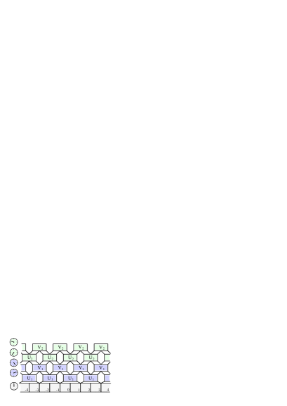
Figure 1: Two timesteps of the ccQCA. The clocks indicate the the time before and after application of the unitaries for comparison to FIG. 2.

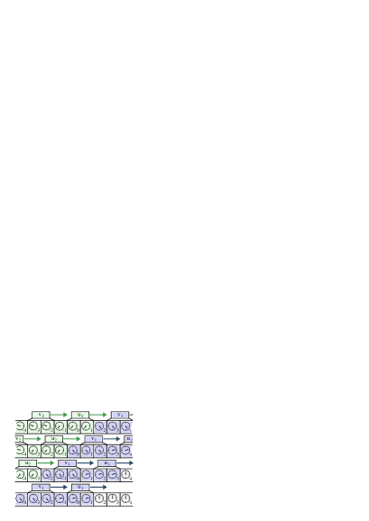
Figure 2: Four timesteps of the autonomous QCA. As the cells are updated sequentially, the clocks indicate the local time of the cells corresponding to the time of the ccQCA.

.2 Explicit construction

.2.1 Construct circuit of controlled partial $\sigma_{y}$

There is a two-qubit gate which, if not constrained to act always on neighbouring qubits but allowed to act on qubits within arbitrary range, serves as universal for computation within the standard gate model. This gate is defined as

$$G~{}=~{}\left(\begin{array}[]{cccc}1&0&0&0\\ 0&1&0&0\\ 0&0&\frac{1}{\sqrt{2}}&\frac{-1}{\sqrt{2}}\\ 0&0&\frac{1}{\sqrt{2}}&\frac{1}{\sqrt{2}}\end{array}\right)$$ (1)

in the computational basis, $\{\,|00\rangle,|01\rangle,|10\rangle,|11\rangle\,\}$. It performs a $\pi/4$ rotation on one qubit conditioned on the setting of another. To see that this gate is universal, it suffices to show that by use of simple (computational-basis) ancillæ, one can simulate both the Hadamard and the Toffoli gates, according to the well-known results of lit:QGC .

.2.2 Construct qubit ccQCA

Consider a ccQCA on a 1-dimensional qubit lattice that allows the use of four different kinds of QCA-homomorphisms as described below. To show how this ccQCA can be used to simulate an arbitrary gate model circuit whose gates are of the kind $G$ (1), we will think of the ccQCA’s qubits as belonging to three interleaved 1-dimensional lattices, and label them accordingly as $d_{i},a_{i},h_{i}$ with $i\in\mathbbm{Z}$. We will load the $d$-band with input corresponding to the input of the gate array being simulated, initialising its unused qubits to $|0\rangle$. The $a$-band will be used as ‘ancilla space’ and should be initialised to $|0\rangle$ everywhere. The $h$-band is used to break spatial symmetry of the dynamics, and should contain a single ‘pointer’ $|1\rangle$ with the rest of its qubits containing $|0\rangle$. The four families of homomorphisms we allow are

$$A_{i}=\prod_{x\in\mathbbm{Z}}G(h_{x},a_{x+i}), B_{i}=\prod_{x\in\mathbbm{Z}}G(h_{x},d_{x+i}),$$

$$C_{i}=\prod_{x\in\mathbbm{Z}}G(d_{x},a_{x+i}), D_{i}=\prod_{x\in\mathbbm{Z}}G(a_{x},d_{x+i}),$$

(see FIG.3) and we simulate the gate $G(d_{i},d_{j})$ by the classically controlled sequence (reading right to left)

$$A_{0}^{7}\cdot C_{-i}^{7}\cdot B_{i}^{6}\cdot C_{-i}\cdot D_{j}\cdot C_{-i}^{7}\cdot B_{i}^{2}\cdot C_{-i}\cdot A_{0}=G(d_{i},d_{j}).$$ (3)

The reader may check that this effects the required transformation on the $d$-band, restoring the other two bands to their original configurations, assuming the initialisations described above. Of course, a clever compiler would find ways of simulating a given circuit that are far more efficient than repeated application of this technique.

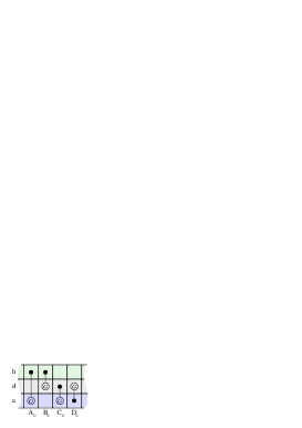
Figure 3: Structure of the ‘three band’ QCA with pointer, data and ancilla band. Localisation of the homomorphisms (.2.2) are indicated.

.2.3 Construct nearest neighbour qubit ccQCA

The ccQCA described above employs operations with arbitrarily large neighbourhood. With additional neighbour-swap operations we can first move two bands to the required interband-distance $i$, then apply a cellwise $G$-operation ($A_{0},B_{0},C_{0}$, or $D_{0}$) and finally shift back, in order to implement all operations (.2.2) with a nearest neighbour ccQCA. Moreover, the interband $G$-operations are quite similar, which suggests to interleave the three bands into a single qubit band labelled $q_{i},i\in\mathbbm{Z}$

$$(..,q_{-2},q_{-1},q_{0},q_{1},q_{2},..)=(..,a_{-1},h_{-1},d_{0},a_{0},h_{0},..).$$

A sufficient set of operations is then given by

$$E_{i} = \prod_{x\in\mathbbm{Z}}\mbox{Swap}(q_{3x+i},q_{3x+i+1}),$$

$$F_{i} = \prod_{x\in\mathbbm{Z}}G(q_{3x+i},q_{3x+i+1}),$$ (4)

for $i\in\{\,0,1,2\,\}$. It should be noted that it suffices to move two bands relative to each other, since the homomorphisms of (.2.2) act non-trivially on only two bands at a time.

.2.4 Construct universal nearest-neighbour QCA

The homomorphisms of the ccQCA already work on non-overlapping neighbourhoods, and so there is no need for further Margolus decomposition here. Next we offer a design which further minimizes the Hilbert space dimension of the cells of which the QCA will be composed.

Take a 1-dimensional lattice of qudits labelled $c_{i}$ (for $i\in\mathbbm{Z}$) of single cell dimension $d=12$, and regard these as incorporating one qutrit cell of the program band $t_{i}$ with two qubit cells $q_{2i}$ and $q_{2i+1}$ from the data band. The cell $c_{i}$ we define explicitly as the tensor product

$$c_{i}=t_{i}\otimes q_{2i}\otimes q_{2i+1}.$$ (5)

(Identification of data cells is indicated in FIG. 4) As before, it is not necessary to have any ‘fine control’ over the relative motion of the two sub-bands; rather we simply allow one to pass by the other with an invariant velocity. This is again achieved by decomposing the QCA transformation step into two parts, a unitary and a shift:

$$U\colon~{}\mathbbm{C}^{12}\rightarrow\mathbbm{C}^{12}\mbox{ acting on every cell simultaneously,}$$

$$S\colon~{}\left(\begin{array}[]{rcl}t_{i}&\mapsto&t_{i+1}\\ q_{i}&\mapsto&q_{i-1}\end{array}\right)\mbox{ sliding the bands relatively.~{}~{}~{}~{}}$$ (8)

To simulate the nearest-neighbour ccQCA, we will interpret the data band $q_{i}$ exactly as before, but the program band $t_{i}$ must be initialised so as to execute the appropriate transformations on the data band as the two bands slide past one another. At initialisation, the cells $i>0$ will be used to hold the non-zero content of the data band in their qubits, while the cells $i<0$ will be used to hold the program band in their qutrits. We will initialise the $t_{i}$ in the computational basis, and the $U$ operation will be defined to leave these qutrits invariant. Specifically, $t_{i}=|0\rangle$ will cause no transformation, $t_{i}=|1\rangle$ will cause a swap of data between $q_{2i}$ and $q_{2i+1}$, and $t_{i}=|2\rangle$ will cause the transformation $G(q_{2i},q_{2i+1})$ described in (1).

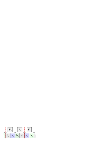
Figure 4: Structure of the autonomous QCA. Indicated are three cells with one program qutrit and two data qubits each; identification of the data qubits corresponding to FIG. 3.

Each of the homomorphisms of (.2.3) is simulated not by one QCA timestep but by three neighbouring qutrits sliding past all of the data-bearing qubits. Specifically, the program-segment $|t_{3i}\,t_{3i+1}\,t_{3i+2}\rangle\equiv|100\rangle$ will simulate the homomorphism $E_{0}$, the program-segments $|010\rangle$ and $|001\rangle$ will simulate the homomorphisms $E_{2}$ and $E_{1}$. Likewise, the program-segments $|200\rangle$, $|020\rangle$, $|002\rangle$, will simulate the homomorphisms $F_{0}$, $F_{2}$, $F_{1}$, respectively. The cells with negative index may be initialised with program-segments of these kinds in order to induce the desired transformations on the data. The computation output may be read (in computational basis) any time after the content of the program band has moved past the content of the data band.

To show that this simulation is efficient, one needs to estimate the necessary resources. Consider a quantum gate circuit (QGC) of Space_QGC qubit-wires and Time_QGC $G$-gates. In the first simulation step, the resources of the ccQCA depend linearly on the corresponding QGC resources. The use of swap gates in the next step increases the time; the encoding of the program into the program band increases the space, so one ends up with an estimate for the autonomous QCA of

$$\mbox{{Time}}_{QCA}=\mathcal{O}(\mbox{{Time}}_{QGC}\cdot\mbox{{Space}}_{QGC}),$$

$$\mbox{{Space}}_{QCA}=\mathcal{O}(\mbox{{Time}}_{QGC}\cdot\mbox{{Space}}_{QGC}).$$ (9)

The resources depend polynomially on the given QGC, so the simulation is efficient.

.3 Acknowledgements

DJS is sponsored by CESG. RFW acknowledges support from the QUPRODIS network of the EU.

References

- (1) B. Schumacher and R.F. Werner, Reversible quantum cellular automata, (quant-ph/0405174)
- (2) J. Watrous, On one-dimensional quantum cellular automata, in Proceedings of the 36th Annual Symposium on Foundations of Computer Science (1995) pp. 528–537
- (3) R. Raussendorf, A quantum cellular automaton for universal quantum computation, Phys. Rev. A 72, 022301 (2005)
- (4) A. Y. Vlasov, Programmable Quantum Networks with Pure States, (quant-ph/0503230)
- (5) S. C. Benjamin, S. Bose, Quantum Computing in Arrays Coupled by ‘Always On’ Interactions, Phys. Rev. A 70, 032314 (2004)
- (6) I. Bloch, Ultracold Quantum Gases in Optical Lattices , Nature Physics 1 (2005) pp. 23–30
- (7) D. Aharonov, A simple Proof that Toffoli and Hadamard are Quantum Universal, (quant-ph/0301040)