Quantum algorithm for optical template recognition with noise filtering

Abstract

We propose a probabilistic quantum algorithm that decides whether a monochrome picture matches a given template (or one out of a set of templates). As a major advantage to classical pattern recognition, the algorithm just requires a few incident photons and is thus suitable for very sensitive pictures (similar to the Elitzur-Vaidman problem). Furthermore, for a $2^{n}\times 2^{m}$ image, ${\cal O}(n+m)$ qubits are sufficient. Using the quantum Fourier transform, it is possible to improve the fault tolerance of the quantum algorithm by filtering out small-scale noise in the picture. For example images with $512\times 512$ pixels, we have numerically simulated the unitary operations in order to demonstrate the applicability of the algorithm and to analyze its fault tolerance.

I Introduction

It is well known that quantum computers are suited to solving certain classes of problems much better than classical computers. A prominent example is Shor’s algorithm shor1997 for factoring an integer number with an effort that grows polynomially in the number of its digits, which is believed to be classically impossible. A further impressive example is Grovers algorithm grover1997 for finding an item in an unsorted database: There, the effort grows only as the square-root $\sqrt{N}$ of the number $N$ of database entries on a quantum computer, whereas it grows with $N$ on a classical computer. In addition, there are further black box problems such as the Deutsch deutsch1985 and the Deutsch-Josza algorithm deutsch1992 as well as others elitzur1993 ; simon1997 ; bernstein1997 (for an overview see e.g., nielsen2000 ).

The possible speedup of quantum algorithms is essentially enabled by the feature of quantum parallelism. This parallelism permits to calculate with a superposition of states on a quantum computer, which is not possible on classical computers. The first quantum computers have already been constructed. For example, Shor’s algorithm has been used on an NMR quantum computer vandersypen2001 to factorize the number 15. This is certainly not impressive if one considers the smallness of the number but nevertheless serves as a proof of principle.

However, there exists a plethora of further classically challenging problems such as e.g., pattern recognition fukunaga1972 , which can also benefit from the application of quantum algorithms horn2002 ; sasaki ; trugenberger . It has already been demonstrated that quantum parallelism can be exploited to identify and localize a regular simple pattern schuetzhold2003 within an otherwise unstructured picture. Here, we will present a probabilistic quantum algorithm that is capable of recognizing an arbitrary image (even in the presence of noise at a moderate level) after shining a few photons on the picture. In contrast to previous pattern matching approaches (see, e.g., trugenberger ), it does not require the copying of quantum states (which is only possible probabilistically for general states) and enables a (probabilistically) non-destructive measurement, cf. elitzur1993 .

II Problem Definition

Following the problem description of schuetzhold2003 , let us consider a large rectangular $N_{x}\times N_{y}$ array of unit cells that may either be black (absorptive) or white (reflective). To allow for a binary representation, we will consider cases where the number of array cells in every dimension are powers of 2, i.e., $\log_{2}N_{x/y}=n_{x/y}$ with integers $n_{x/y}$. Further-on, we will denote the pixels in the array that are reflective (white) as points.

The problem consists of recognizing whether the pattern in the array matches a given template (for example, a letter of an alphabet). Note that this slightly differs from template matching discussed e.g., in trugenberger ; sasaki , where a template is to be found that optimally matches the given unknown quantum state. With using varying templates however, one can evidently establish a relation between these problems. Some aspects of the presented quantum algorithm will be similar to the discrimination problem of known quantum states bergou2004 via suitably chosen positive operator valued measures (POVM), which will be discussed in section VII.

The classical approach to measure the displayed pattern on the array would be to shine light (consisting of many, say ${\cal O}\{{N_{x}\times N_{y}}\}$, photons) on the array and to measure absorption and transmission accordingly. However, in the case we consider here, the array is also assumed to be very sensitive (imagine, for example, an exposed but not yet developed film or a pattern of partially fluorescent ions in a Paul trap), such that each absorbed photon causes a certain amount of damage. Evidently, the classical measurement approach would significantly disturb the system.

One might worry that the momentum of the reflected photon (recoil) also disturbs the picture, but this effect will be extremely small if the mass of a pixel is sufficiently big. Alternatively, one might imagine the reflective pixels to be transparent and to place a mirror behind the array.

Then, a quantum algorithm can cope with such a task: The feature of quantum parallelism can be exploited by storing the relevant information of the image in a quantum superposition state with using just a single photon and not (or only very little) destroying the image. The task is thus similar to the Elitzur-Vaidman problem elitzur1993 , which allows for testing for the existence of an object without any energy-momentum exchange.

III Read-Out Scheme

Generally, the coordinates $(x,y)$ of a pixel in the image can be written in their binary representation

$$x={x_{1}}\otimes\ldots\otimes{x_{n_{x}}} y={y_{1}}\otimes\ldots\otimes{y_{n_{y}}}\,,$$ (1)

where $x_{i}$ and $y_{j}$ denote the $i$-th and $j$-th bit of $x$ and $y$, respectively, i.e., $x=x_{1}2^{n_{x}-1}+x_{2}2^{n_{x}-2}+\ldots+x_{n_{x}}$. Regarding these coordinates $(x,y)$ as control qubits $|x\rangle=|x_{1}\rangle|x_{2}\rangle\ldots|x_{n_{x}}\rangle$, the photon probing the image can be entangled with the coordinates in the following way:

The photon passes through a series of quantum controlled refractors $R_{n_{x}}^{x}\ldots R_{1}^{x}R_{n_{y}}^{y}\ldots R_{1}^{y}$ that effectively displace the photon by defined distances $\Delta x_{i}$ or $\Delta y_{i}$, if the control qubit $|x_{i}\rangle$ or $|y_{i}\rangle$ is in the state $|1\rangle$ and leave it unaffected if the control bit is in the state $|0\rangle$. By choosing the displacement of the refractor $R_{i}^{x}$ as $\Delta x_{i}=2^{i}\Delta x_{0}$ (and likewise for the other refractors $R_{i}^{y}$), the final displacement of the photon corresponds to the coordinates $(x,y)$ which encode the position of a single image pixel.

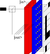
Figure 1: [Color Online] Left: Illustration of a series of three quantum-controlled refractors required for an 8-pixel one-dimensional array. A photon created by the source (box in the left) passes the refractor series, interacts with the pixel array and takes – if reflected – the reverse path. Depending on the value of the control qubits $|x_{i}\rangle$, the refraction index of the medium is changed, which effectively produces a displacement of the photon. Right: Schematic representation of the two-dimensional configuration (exemplified for an $8\times 4$ array). The first three refractors generate the displacement in $x$-direction (for 8 pixels) and the remaining two act in the $y$-direction (for 4 pixels).

In a laboratory setup, this could for example be realized by using a varying refractor thickness, see figure 1 left panel. For quantum controlled devices, one can generate superposition states of several pixel positions in the image as control qubits. Storing these bits in a coherent superposition state containing all pixels with equal amplitudes, a single photon can be forced to interact simultaneously and uniformly with the complete array.

One should be aware that this causes a strong entanglement between the photon position and the control qubits. Thus, any measurement on the photon would affect the refractor control qubits as well and completely decohere them. The interaction of the photon with the image corresponds to absorption or reflection. In case of (perpendicular) reflection, the photon will reverse its original path (this is enforced by the entanglement with the refractor control qubits) and after passing through all refractors again, all information about the way of the photon (given that it was reflected) is lost. Thus, the entanglement with the control qubits is partially removed (quantum eraser) and we obtain a coherent superposition of the reflecting pixels (points). In the other case (absorption), the entanglement cannot be removed, and the algorithm fails – i.e., one has to send another photon if permitted by the fragility of the quantum array. As a formal simplification, one can consider the action of the configuration of the setup in figure 1 as a quantum black box:

$${\mathcal{B}}\;:\;|x\rangle\otimes|y\rangle\otimes|0\rangle\,\to\,|x\rangle\otimes|y\rangle\otimes|f(x,y)\rangle\,,$$ (2)

which encodes the output in the characteristic function $f(x,y)$ of the image. The function $f(x,y)$ takes the value 1 if the pixel $x\otimes y$ is reflective (i.e., if $|x\rangle\otimes|y\rangle$ encodes a point) and 0 if the pixel is black (i.e., if the photon is absorbed). If the control qubits on the refractors are initially prepared in a superposition state (e.g., acting Hadamard gates on each qubit), the characteristic function $f(x,y)$ of the image is tested for all pixels simultaneously

$${\mathcal{B}}\left[{\mathcal{H}}^{(n_{x})}|0^{(n_{x})}\rangle\otimes{\mathcal{H}}^{(n_{y})}|0^{(n_{y})}\rangle\otimes|0\rangle\right]=$$

$$\frac{1}{\sqrt{N_{x}N_{y}}}\sum_{x=0}^{N_{x}-1}\sum_{y=0}^{N_{y}-1}|x\rangle\otimes|y\rangle\otimes|f(x,y)\rangle\,.$$ (3)

Measuring the third register (i.e., the existence of a reflected photon) and obtaining $|1\rangle$ as a result prepares the quantum state as an uniform superposition of all points in the image. The other outcome ($|0\rangle$) corresponds to the absorption of the photon and would lead to entanglement between the refractor control qubits and the image. Thus, with the outcome $|1\rangle$ (outgoing photon) one has prepared a quantum state (in the refractor control qubits) that is suitable for performing further calculations. An alternative scheme based on linear optics, which could be applied if the image is not too large, is discussed in the Appendix. Note that this scheme has the advantage that the image does not have to be loaded into a possibly fragile quantum memory (cf. trugenberger ; sasaki ).

IV Quantum Algorithm

After extracting the superposition state containing all points of the image

$$|\Psi\rangle=\sum_{x=0}^{N_{x}-1}\sum_{y=0}^{N_{y}-1}\frac{f(x,y)}{\sqrt{M}}|x\rangle|y\rangle=\sum\limits_{(x,y)\in\rm image}\frac{|x,y\rangle}{\sqrt{M}}\,,$$ (4)

where $M$ with $1\ll M<N_{x}N_{y}$ denotes the total number of points, one has to decide whether it corresponds to a given template.

Obviously, a $N_{x}\times N_{y}$ array (in black and white) could contain $2^{N_{x}N_{y}}$ different images – but the Hilbert space of all possible quantum state has merely $N_{x}N_{y}=2^{n_{x}+n_{y}}$ dimensions. Hence different images will not correspond to orthogonal quantum states in general and thus it is – even in the absence of noise – not possible to distinguish them with certainty, i.e., the presented quantum algorithm can only work probabilistically.

The problem of efficiently discriminating non-orthogonal quantum states has been studied extensively and is usually formulated within the framework of positive operator valued measures (POVM): Given a quantum state out of a set of perfectly known (non-orthogonal) quantum states, it is possible to construct a POVM which decides probabilistically which one of these states it is with minimum error probability, see section VII. However, the design of a suitable POVM will be – especially in the case of large images (high-dimensional Hilbert-spaces) with more than two possible quantum states – quite demanding in general bergou2004 ; ariano2005 . In addition, if the quantum states are not known exactly – e.g., in the presence of perturbations and noise – the construction of the optimal POVM is even more complicated. Finally, the physical realization of such an optimal POVM will also be quite demanding in general and can easily destroy part of the speed-up of the quantum algorithm. Therefore, we propose a different procedure that shifts the effort from designing a suitable POVM towards the implementation of a quantum oracle gate (in an inverse application of Grovers algorithm).

Using the characteristic function $f(x,y)$ of the image (which yields 1 for the marked items, i.e., points of the image, and 0 otherwise) as an oracle, a Grover iteration generates a rotation in the two-dimensional sub-space of the Hilbert space spanned by the coherent superpositions of all numbers $|s\rangle={\mathcal{H}}^{(n_{x})}|0^{(n_{x})}\rangle\otimes{\mathcal{H}}^{(n_{y})}|0^{(n_{y})}\rangle$ on the one hand and the numbers of the marked items, i.e., the state $|\Psi\rangle$ in the above equation, on the other hand. Since there are $M$ solutions to this search problem,

$$R=\left\lceil{\frac{\pi}{4}\sqrt{\frac{N_{x}N_{y}}{M}}}\right\rceil$$ (5)

inverse Grover iterations will rotate the original state $|\Psi\rangle$ in Eq. (4) into the total superposition state $|s\rangle$, or at least close to it (discretization error, cf. discretization ). After application of a Hadamard gate to each of the qubits, the resulting state would be $|0^{(n_{x})}\rangle\otimes|0^{(n_{y})}\rangle$. If the image indeed perfectly equals the template – i.e., if their characteristic functions coincide – and if the Grover iterations were assumed to be perfect (no discretization error), the state $|\Psi\rangle$ in Eq. (4) prepared after measuring the returning photon would be unitarily transformed into the final state $|0^{(n_{x})}\rangle\otimes|0^{(n_{y})}\rangle$. Consequently, a measurement in the computational basis would yield zeros for all bits.

If the image differs from the template (and assuming a perfect Grover rotation discretization ), the probability of ending up in the final state $|0^{(n_{x})}\rangle\otimes|0^{(n_{y})}\rangle$ would be given by the overlap of the characteristic functions of the template $f(x,y)$ and the image $f^{\prime}(x,y)$

$$p=\frac{1}{MM^{\prime}}\left|\sum_{x=0}^{N_{x}-1}\sum_{y=0}^{N_{y}-1}f(x,y)f^{\prime}(x,y)\right|^{2}$$ (6)

since all involved operations were unitary and hence probability conserving. Since this overlap determines how similar image and template are, measuring all qubits at the end and obtaining zero everywhere is a strong indication that the image equals the template or at least is very similar to it. Obtaining 1 somewhere, on the other hand, indicates that the image does not equal the template with high probability discretization . As usual, the result can be made more decisive by repeating the whole algorithm.

V Noise Filtering

So far, the input state $|\Psi\rangle$ was assumed to be perfect. However, in reality neither the realization of the image in the array nor the reflection and absorption properties of the image pixels can be assumed as perfect. Therefore, the basic algorithm described above can be improved using the quantum Fourier transform to reduce possible perturbations: As in classical pattern recognition, one can perform a cutoff of large wave-numbers, which reduces noise such as pixel defects. In a quantum algorithm, such a cutoff has to be implemented in a suitable way – just measuring the $k$-value and subsequently deciding whether it lies above of below the cutoff does not work, since a hard $k$-measurement completely decoheres the quantum state. Therefore, a noise-filter should be realized via the measurement of an ancilla qubit which has been coupled to the control qubits: To this end, we introduce a unitary noise-filter operator

$${\mathcal{N}}\left[|k_{x}\rangle\otimes|k_{y}\rangle\otimes|0\rangle\right]=$$

$$|k_{x}\rangle\otimes|k_{y}\rangle\otimes\left\{\cos[\vartheta(k_{x},k_{y})]|1\rangle+\sin[\vartheta(k_{x},k_{y})]|0\rangle\right\}\,,$$ (7)

with a suitably chosen noise-filter function $\vartheta(k_{x},k_{y})$. Measuring the last register and obtaining $|1\rangle$ performs the desired cutoff in frequency space.

Let $M_{\rm tp}$ denote the number of template points and $M_{\rm im}\approx M_{\rm tp}$ the number of image points. Then, the quantum algorithm can be summarized as follows (compare also figure 2):

1. initialize the state vector with uniform superpositions in $x$ and $y$ as well as two ancilla qubits
   ${|\Psi_{1}\rangle=\mathcal{H}}^{(n_{x})}|0^{n_{x}}\rangle\otimes{\mathcal{H}}^{(n_{y})}|0^{n_{y}}\rangle\otimes|0\rangle\otimes|0\rangle$

2. apply the black box with the first ancilla qubit
   ${|\Psi_{2}\rangle={\mathcal{B}}|\Psi_{1}\rangle}$

3. measure the first ancilla qubit and proceed after obtaining the outcome $|1\rangle$
   $|\Psi_{3}\rangle\stackrel{{\scriptstyle|1\rangle}}{{=}}M_{\rm im}^{-1/2}\sum\limits_{(x,y)\in\rm image}|x\rangle\otimes|y\rangle\otimes|1\rangle\otimes|0\rangle$

4. perform quantum Fourier transform in $|x\rangle$ and $|y\rangle$
   $|\Psi_{4}\rangle={\cal QFT}_{x,y}|\Psi_{3}\rangle$

5. apply noise filter operator with second ancilla
   $|\Psi_{5}\rangle={\mathcal{N}}|\Psi_{4}\rangle$

6. measure the second ancilla qubit and proceed after obtaining the outcome $|1\rangle$
   $|\Psi_{6}\rangle\stackrel{{\scriptstyle|1\rangle}}{{=}}\sum_{k_{x},k_{y}}\tilde{f}_{\rm cut}(k_{x},k_{y})|k_{x}\rangle\otimes|k_{y}\rangle\otimes|1\rangle\otimes|1\rangle$
   with $\tilde{f}_{\rm cut}(k_{x},k_{y})=\tilde{f}(k_{x},k_{y})\cos[\vartheta(k_{x},k_{y})]$

7. perform the inverse quantum Fourier transform
   $|\Psi_{7}\rangle={\cal QFT}_{x,y}^{\dagger}|\Psi_{6}\rangle$

8. perform $R=\left\lceil{\frac{\pi}{4}\sqrt{\frac{N_{x}N_{y}}{M_{\rm tp}}}}\right\rceil$ inverse Grover iterations
   $|\Psi_{8}\rangle={\cal G}^{-R}|\Psi_{7}\rangle$

9. apply Hadamard gates on non-ancilla qubits
   $|\Psi_{9}\rangle={\mathcal{H}}^{(n_{x})}\otimes{\mathcal{H}}^{(n_{y})}|\Psi_{8}\rangle$

10. measure final state in computational basis
    $|\Psi_{9}\rangle\stackrel{{\scriptstyle?}}{{=}}|0^{(n_{x})}\rangle\otimes|0^{(n_{y})}\rangle\otimes|1\rangle\otimes|1\rangle$

The algorithm fails when measurement of one of the ancilla qubits yields $|0\rangle$, i.e., if the photon is absorbed or if a projection onto the wrong $k$-values is performed.

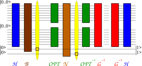
Figure 2: [Color Online] Quantum circuit of the template matching algorithm for 14 control qubits (7 for $x$ and $y$ respectively) plus 2 ancilla qubits (ancilla qubit values shown for a successful run).

The probability of obtaining finding the system in the state $|0\ldots 0\rangle\otimes|1\rangle\otimes|1\rangle$ as the result of the last measurement corresponds to the probability of template matching, i.e., given a template such as the letter A and an initial state such as the (noise-perturbed) state $|B\rangle$, the quantum algorithm decides whether the template is matched or not discretization .

VI Algorithmic Performance

Starting from a possibly noise-perturbed initial state as prepared by step 3 of the quantum algorithm, we have numerically simulated the action of the corresponding unitary gates and measurements for the $512\times 512$ example arrays in figure 3. As the number of allowed states increases exponentially with the number of simulated $n_{x}+n_{y}$ qubits, the numerical simulations would involve $2^{n_{x}+n_{y}}\times 2^{n_{x}+n_{y}}$ matrices which do not fit into the main memory. Fortunately, the involved unitary operations can be expanded into combinations of one or two qubit operations nielsen2000 , which can be calculated. Thus, the whole algorithm for pattern recognition for $n_{x}+n_{y}=18$ qubits runs in a time of few seconds. As a noise-filter function a sharp cutoff was used, i.e.,

$$\vartheta(k_{x},k_{y})=\left\{\begin{array}[]{ccc}0&:&0<\sqrt{k_{x}^{2}+k_{y}^{2}}<k_{\rm max}\\ \pi/2&:&\mbox{otherwise}\end{array}\right.\,,$$ (10)

which leads to a simple projection on the allowed $k$-values. In addition to the high-frequency ($k\geq k_{\rm max}$) components, it can be advantageous to remove the $k_{x}=k_{y}=0$ component as well, especially if the noise significantly changes the total number of points in the image.

The computational complexity of the algorithm depends on the total number of pixels and on the number of points in the template. The Hadamard gates and the quantum controlled refractors require ${\cal O}\{{n_{x}+n_{y}}\}$ operations and the quantum Fourier transforms involve ${\cal O}\{{n_{x}^{2}+n_{y}^{2}}\}$ gates. The necessary number of Grover iterations depends on the size of the template $R={\cal O}\{{\sqrt{N_{x}N_{y}/M_{\rm tp}}}\}$, and the number of involved gates per Grover iteration depends on the physical realization of the oracle function $f(x,y)$. Many template points (e.g., bold and large letters) lower the number of required Grover iterations.

Similarly, one has to estimate the failure probability, i.e., how often measurement of one of the ancilla bits yields zero. The probability for the photons to be reflected (first ancilla) is given by the ratio of the image size (number of points) over the total area of the array (number of pixels), i.e., many image points are favorable (similar to the above argument). For the second ancilla the failure probability depends on the amplitudes of the removed $k$-values and thus roughly on the amount of noise and the number of fine details in the image.

For specific templates we have made our algorithm explicit: With a given template A or B (cf. figure 3 top panels), we numerically calculated the recognition probability for all the possible combinations (image A and template B versus template A etc.) for various noise levels (cf. figure 3 lower panels).

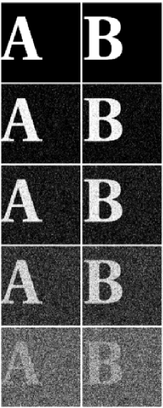
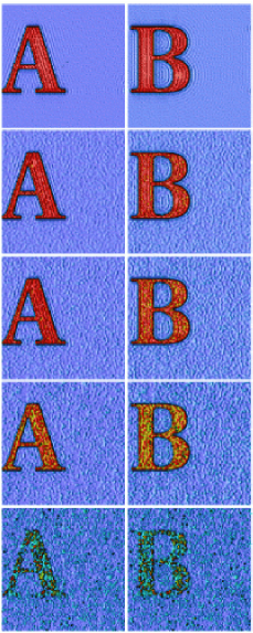
Figure 3: [Color Online] Left: Images of the input states ($512\times 512$) with various noise levels. From top to bottom the image pixels of the initial state have been inverted with a probability of 0%, 5%, 10%, 20%, and 40%, respectively. Right: Panels show the distribution of the squared amplitude of the inverse of the Fourier-smoothed images (i.e., after step 6 of the quantum algorithm). Only $k$-values with $0<k<40$ have been kept. All amplitudes larger than half the maximum amplitude in every image are shown in red, whereas the thin black isoline encodes the quarter of the maximum amplitude.

The results of the numerical simulations are shown in figure 4. The slight differences between the letters A and B result from the different numbers of image points occupied by the two templates (discretization error discretization of the Grover iterations etc.), as has been checked by applying the algorithm to a different (more symmetric) font. An important quantity is the the discrimination ability of the algorithm, i.e., the capability to distinguish between the alternatives in the given alphabet A and B, see figure 4. A rough measure for the discrimination ability is given by the difference between the acceptance probability when the input state corresponds to the template (circle symbols) and the acceptance probability when the input state does not match the template (square symbols). Without noise, this difference is over 70% and even with 40% noise, the discrimination ability is still significant (around 30%), provided that a noise filter is applied. Without noise filter, the discrimination ability decreases much faster.

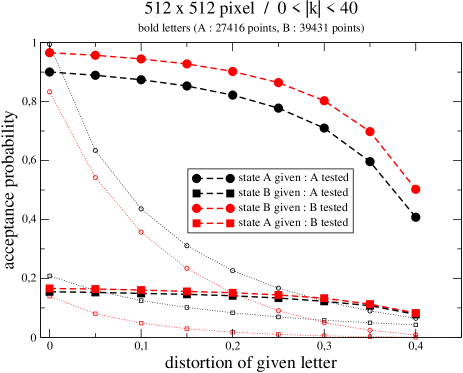
Figure 4: [Color Online] Probability to recognize the initial state as the template versus noise level. Small hollow symbols represent results without noise-filter applied.

VII Failure probability

As already mentioned in sections II and IV, the task in section IV is similar to the well-known discrimination problem: Given a quantum state out of a set of perfectly known (non-orthogonal) quantum states, it is possible to construct a positive operator valued measure (POVM) which decides which one of these states it is. Since non-orthogonal states cannot be distinguished with certainty, such a POVM measurement can never be performed without any errors or ambiguities nielsen2000 . However, a POVM can be optimal in the sense that it minimizes the error probability. Another optimal choice would be a POVM that never leads to an error but sometimes to inconclusive results, but this choice is not suitable for quantum states that are not known exactly.

The explicit construction of the POVM operator has only been possible for a few simple cases. For example, if only the two states $\rho_{A}=|A\rangle\langle A|$ and $\rho_{B}=|B\rangle\langle B|$ can occur with probabilities $p_{A}+p_{B}=1$, an optimal POVM can be constructed helstrom1976 ; bergou2004 via the projectors on the eigenvectors of the operator

$$\Lambda=p_{A}\rho_{A}-p_{B}\rho_{B}\,.$$ (11)

Keeping in mind that the dimension of the Hilbert space grows exponentially, finding the corresponding eigenvectors already becomes a computationally challenging task. More important however is the difficulty that in an experiment, the measurement of such an observable must be implemented.

Associated with an optimal POVM one obtains the minimum error in distinguishing between the states $|A\rangle$ and $|B\rangle$ from the Helstrom formula helstrom1976

$$P_{\rm err}=\frac{1}{2}\left(1-\sqrt{1-4p_{A}p_{B}\left|\langle A|B\rangle\right|^{2}}\right)\,.$$ (12)

Of course, such a simple construction is only possible if non-perturbed quantum states are used. Nevertheless, one can compare the error probability of the quantum algorithm in case of quantum state discrimination with the optimal one, see figure 5. Without noise, the error probability of the quantum algorithm lies only a few percent above the lower bound of about 6%. In the presence of noise, the quantum algorithm is of course more likely to make mistakes, but then it should not be compared with the POVM bound since this was derived assuming exactly known quantum states. For comparison, we plotted the performance of the naive POVMs containing the projector expectation values $|A\rangle\langle A|$ and $|B\rangle\langle B|$ (dotted lines), respectively, which are clearly inferior to the presented quantum algorithm in the presence of noise.

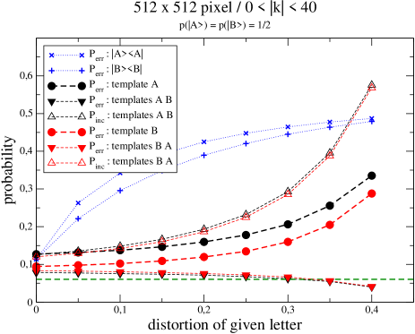
Figure 5: [Color Online] Error probability of the quantum algorithm when applied to state discrimination for equally distributed states $p_{A}=p_{B}=1/2$. The dashed horizontal line corresponds to the minimum error (12) for unperturbed states $|A\rangle$, $|B\rangle$ (as in figure 3 top left panels). The errors of the quantum algorithm (large circle symbols) correspond to the averaged failure probabilities in figure 4 with the respective template. For comparison, the error probabilities obtained from the expectation values of the projection operators $|A\rangle\langle A|$ and $|B\rangle\langle B|$ have been added (small symbols). At the price of introducing an inconclusive result (hollow triangle symbols), the probability of obtaining a conclusive but wrong result can be lowered even further (filled triangle symbols), see section VIII. Note that the POVM bound does not apply in this case and that the decline of this error probability with increasing noise is due to the fact that the probability of obtaining a conclusive result decreases also. The conditional probability of getting the wrong answer provided that the algorithm arrived at a conclusive result of course increases with noise – but is still below the other curves (not shown).

As will be discussed in the following section, it is possible to reduce the error probability even further at the expense of introducing an inconclusive result.

VIII Algorithmic Extensions

Note that the algorithm is vulnerable to translation, i.e., it does not recognize an image that has been translated in position space compared to the template. To cope with translations, it is necessary to use more than one reflected photon and to analyze the two-photon correlations. After determining the center of mass of the image, for example, one could perform the same algorithm with a template that has been shifted accordingly.

Since the objective is to shine as few photons as possible onto the image, one should try to extract as much information as possible from single measurements. Unfortunately, after a complete measurement of all the qubits separately, the full quantum state has been projected onto the outcome and no information is left. However, in order to accept or reject the hypothesis of a given template, we do not need to measure all the qubits. It is completely sufficient to ask the question “Are all the non-ancilla qubits in the state $|0\rangle$ or not?” Alternatively, one could also construct a unitary operator (as with the noise-filter operator $\mathcal{N}$) that uses another ancilla qubit to answer this question. If the answer by measurement is “yes”, we have accepted the hypothesis (probabilistically) and the full quantum state has been projected onto the state $|0^{(n_{x})}\rangle\otimes|0^{(n_{y})}\rangle\otimes|1\rangle\otimes|1\rangle$. However, if the answer is “no” and we have rejected the hypothesis (again probabilistically), the quantum state has only partially been projected onto the high-dimensional sub-space orthogonal to $|0^{(n_{x})}\rangle\otimes|0^{(n_{y})}\rangle$ and still contains a significant amount of information.

For example, let us assume that we performed the algorithm with the template A and that this hypothesis has been rejected, i.e., not all of the qubits were in the state $|0\rangle$. One possibility for this rejection would be that the input state was $|B\rangle$ or some other quantum state (rejection correct) or that an input state $|A\rangle$ was falsely rejected (either due to strong perturbations or just due to the inherent probabilistic nature, see figure 4). In this case, we can partially undo the operations specific to template A by applying a Hadamard gate onto each qubit again and Grover-rotating back with the template A. Now we may switch to the template B and perform the inverse Grover rotation with the new template B plus the Hadamard gates and measure the outcome. In case the overlap between the images A and B is small enough, the result of this measurement indicates whether the image is probably B and the rejection of A was correct or whether something else happened (e.g., the rejection was erroneous or the image is neither A nor B).

Thus, if the first template had $M_{\rm tp}^{(1)}$ points and the second template had $M_{\rm tp}^{(2)}$ points, we could continue the quantum algorithm as follows

• apply Hadamard gates on non-ancilla qubits
  $|\Psi_{11}\rangle={\mathcal{H}}^{(n_{x})}\otimes{\mathcal{H}}^{(n_{y})}|\Psi_{10}\rangle$

• perform $R=\left\lceil{\frac{\pi}{4}\sqrt{N_{x}N_{y}/M_{\rm tp}^{(1)}}}\right\rceil$ Grover iterations with respect to template A
  
  $|\Psi_{12}\rangle={\mathcal{G}}^{R}_{A}|\Psi_{11}\rangle$

• switch to the second template B and perform
  $R^{\prime}=\left\lceil{\frac{\pi}{4}\sqrt{N_{x}N_{y}/M_{\rm tp}^{(2)}}}\right\rceil$ inverse Grover iterations with respect to template B
  
  $|\Psi_{13}\rangle={\mathcal{G}}^{-R^{\prime}}_{B}|\Psi_{12}\rangle$

• apply Hadamard gates on non-ancilla qubits
  $|\Psi_{14}\rangle={\mathcal{H}}^{(n_{x})}\otimes{\mathcal{H}}^{(n_{y})}|\Psi_{13}\rangle$

• measure final state in computational basis
  $|\Psi_{15}\rangle\stackrel{{\scriptstyle?}}{{=}}|0^{(n_{x})}\rangle\otimes|0^{(n_{y})}\rangle\otimes|1\rangle\otimes|1\rangle$

The measurement at step 10 of the quantum algorithm essentially subtracts the template A from the state. Consequently, in case of a false rejection, the state amplitudes will concentrate on the perturbations of the image and the interference patterns resulting from the Fourier noise-filtering, see figure 6 left panels. The resulting state is then nearly orthogonal to the second hypothesis in general. In case of a correct rejection of the first hypothesis, the state’s squared amplitudes will decrease where the state overlaps with the first template, see figure 6 right panels. Note that here also the different magnitudes of the amplitudes due to the different number of points will in most cases prohibit a complete removal of these amplitudes. In this case, the overlap between the state and the second template will be substantial.

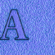
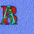
Figure 6: [Color Online] Color-coded distribution of the squared amplitudes of the state after step 12 of the quantum algorithm (rejection of the first hypothesis). Color-coding has been chosen as in figure 3 and all images have been perturbed by 5% initially. From left to right, the combinations have been chosen as follows: (image A & template A), (image B & template B), (image A & template B), (image B & template A).

In this second attempt, the recognition probability for a correct hypothesis is naturally a bit smaller as if the second hypothesis had been tested directly, see large versus small symbols in figure 7. However, this procedure has the advantage, that no further interaction with the image is necessary. A further important advantage is that the probability of falsely recognizing a template is extremely low (large circle symbols in figure 7). This is due to the small overlap of the second hypothesis template and the falsely rejected state vector (compare again figure 6 left panels).

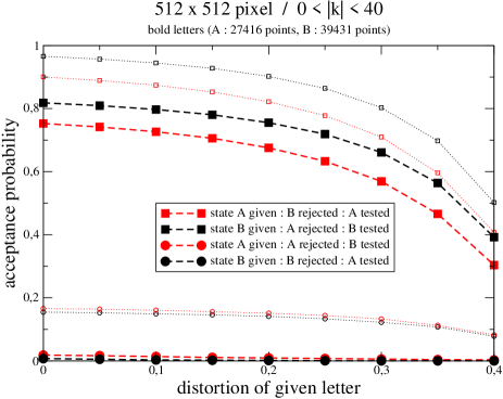
Figure 7: [Color Online] Probability for acceptance of the second hypothesis after rejection of the first one. For comparison, the small hollow symbols (same data as large symbols in figure 4) – corresponding to the acceptance probability if the second hypothesis had been tested as the first one – have been included.

With two templates given, one has only three different outcomes: The first hypothesis can be accepted (1), the first hypothesis can be rejected and the second one is then accepted (2), or none of the hypotheses is accepted (3). In the last case, given that only $|A\rangle$ and $|B\rangle$ can occur, we know that an error must have happened. Consequently, the last outcome must be regarded as inconclusive. With the triangle symbols in figure 5 it becomes visible that with the extended algorithm, the error probability is significantly lowered, whereas the probability for obtaining the inconclusive result rises for strongly perturbed images as one would expect. Consequently, in alphabets containing only few letters, one can identify the letter with a reasonable probability and detect false rejections with high probability – with just a single reflected photon. Thus, the algorithmic extension is similar to a mixture of minimum error and inconclusive POVMs – with the advantage of being applicable to perturbed quantum states.

IX Discussion and Summary

We have demonstrated that a quantum algorithm would be far more effective than a classical computer in template recognition – firstly regarding the number of incident photons and, secondly, in view of the required number of gates.

In case of a successful run, a single photon will suffice to identify a pattern (probabilistically) without disturbing the sensitive image. In this sense, the quantum algorithm realizes a destruction-free measurement (though probabilistically), which is similar to the Elitzur-Vaidman problem elitzur1993 . Even when one takes the finite success probability of the quantum algorithm into account, it still constitutes a major advantage in contrast to classical pattern recognition since a few incident photons suffice. In case of hypothesis rejection, the algorithm can be used to test a different hypothesis without necessitating a further photon interacting with the sensitive array. (Interestingly, the probability of falsely recognizing an input state as the template is much lower in these secondary trials than in the first ones.)

The number of qubits required to run the quantum algorithm on a $2^{n_{x}}\times 2^{n_{y}}$ image is $n_{x}+n_{y}+2$ and the number of gates scales as $n_{x}^{2}+n_{y}^{2}$ for the Quantum Fourier transform, which is also much faster than classical methods. The number of necessary Grover iterations will be rather small ${\cal O}\{{\sqrt{2^{n_{x}+n_{y}}M_{\rm tp}^{-1}}}\}={\cal O}\{{1}\}$, since for reasonable images the number of points is comparable to the number of pixels. Note that the measurements required during the quantum algorithm can also be performed at the end.

However, we have only discussed the algorithm from a theoretical point of view, neglecting many obstacles: For example, we did not discuss the experimental difficulties that are to be expected during an experimental implementation of the required quantum circuit. Apart from the quantum computer itself, the realization of the quantum-controlled refractors poses serious problems. Interestingly, for images of moderate size, the proposed quantum algorithm can in principle be realized with present-day technology using linear optics, see the Appendix. However, the price one has to pay is an exponential scaling of the number of gates etc. Therefore, only the first advantage (i.e., only a few incident photons are required) of the presented quantum algorithm survives in that case.

Despite of these shortcomings, we hope that the presented theoretical discussion of the amazing potential of quantum algorithms will further contribute to the theoretical as well as experimental developments in this fascinating area.

Note added in proof

If it is experimentally feasible to arrange to photon path is a way such that it interacts with the image several times, it is possible to increase the efficiency of the initial state preparation (i.e., suppress the probability for the photon being absorbed) by exploiting the quantum Zeno effect along the lines of P. Kwiat et al., Phys. Rev. Lett. 74, 4763, (1995).

APPENDIX: LINEAR-OPTICS SETUP

Instead of a binary representation, the quantum state can be encoded directly by the path of a single photon in the laboratory. This representation has the advantage that the proposed quantum algorithm can be realized using linear optics elements which are (in principle) already available with present-day technology, see also londero2004 . Unfortunately, this advantage goes along with a serious drawback: The number of elements grows linearly (plus logarithmic corrections) with the number of image pixels, i.e., the computational complexity is exponential instead of polynomial. Hence, this linear-optics scheme is only reasonable for images of moderate size.

Figure 8: Preparation of the initial superposition state $|s\rangle$.
A Hadamard gate on the three-qubit-state $|000\rangle$ is emulated by the combination of beamsplitters (crossed boxes) and mirrors (solid lines), which distribute the amplitude of the incoming photon uniformly on the one-dimensional array (large hatched box, partially absorptive and transmittive).

The initial state $|s\rangle={\mathcal{H}}^{(n_{x})}|0^{(n_{x})}\rangle\otimes{\mathcal{H}}^{(n_{y})}|0^{(n_{y})}\rangle$ can be generated by means of a series of beam splitters as depicted in figure 8 which distribute the photon amplitude uniformly over the array and thus replace the quantum controlled refractors. For a one-dimensional array of $N=2^{n}$ pixels, this scheme necessitates $N-1$ beam splitters.

For this implementation, it is convenient to regard the array as being partially absorptive and transmittive. If the photon passes the array, the quantum state is automatically prepared in a superposition of all points as in equation (4). On the other hand, if the photon is absorbed, no quantum state is created at all, i.e., the existence of a photon corresponds to the measurement of the first auxiliary qubit.

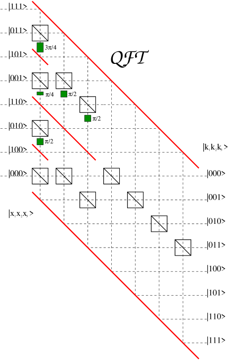
Figure 9: [Color Online] Linear-optical setup for a quantum Fourier transform on a 8-dimensional Hilbert space corresponding to an array with 8 pixels. After interaction with the array, the quantum state (left-hand side) is described by the path of the photon (dashed lines). The quantum Fourier transform is performed using beamsplitters (crossed boxes), mirrors (red solid lines) and phase shifters (green boxes) only. The distances between the beam paths are assumed to be a multiple of the photon wavelength, such that different distances in perpendicular direction do not contribute to the relative phase. The beamsplitters are assumed to act with a phase factor of $-1$ if traversed vertically on a straight line (and without any phase otherwise). The phase shifts (numbers beside boxes) have been adjusted according to equation (APPENDIX: LINEAR-OPTICS SETUP). This scheme only reaches the efficiency of the classical Fast Fourier Transform (FFT). Without the additional phase shifts, the scheme implements a Hadamard gate on all qubits.

Afterwards, a quantum Fourier transform can be performed with the setup in figure 9. In the binary representation $k=\sum\limits_{\ell}k_{\ell}2^{n-\ell}$ and $x=\sum\limits_{j}x_{j}2^{n-j}$, the quantum Fourier transform,

$${\cal QFT}|x\rangle=\frac{1}{\sqrt{N}}\sum_{k=0}^{N-1}\exp\left\{\frac{2\pi ixk}{N}\right\}|k\rangle\,,$$ (13)

possesses the well-known factorization

$${\cal QFT}|x\rangle = \sum_{k=0}^{N-1}|k\rangle\prod_{\ell=1}^{n}\frac{(-1)^{k_{\ell}x_{n-\ell+1}}}{\sqrt{2}}\times$$ (14)

$$\times\prod_{m=2}^{\ell}\exp\left\{2\pi ik_{\ell}x_{n+m-\ell}2^{-m}\right\}\,.$$

For example, one observes for $n=3$ the following phase contributions $\Delta\Phi$

$$\Delta\Phi_{\ell=3} = (-1)^{k_{3}x_{1}}\exp\left\{2\pi ik_{3}\left[x_{2}2^{-2}+x_{3}2^{-3}\right]\right\}$$

$$\Delta\Phi_{\ell=2} = (-1)^{k_{2}x_{2}}\exp\left\{2\pi ik_{2}\left[x_{3}2^{-2}\right]\right\}$$

$$\Delta\Phi_{\ell=1} = (-1)^{k_{1}x_{3}}\,.$$ (15)

By adjusting the beamsplitters such that they automatically induce phase factors of $-1$ if (and only if) traversed vertically on a straight line, we can generate the above phase contributions of $\pi$, i.e., the factors of $(-1)$. The remaining phases (in the above example $3\pi/4$, $\pi/2$, and $\pi/4$) can be implemented by ordinary phase shifters placed in the corresponding paths, cf. figure 9. Note that further mirrors could be used to bring the input states $|x_{1}x_{2}x_{3}\rangle$ in the order of the computational basis. Without these additional phase shifters, the arrangement in figure 9 would correspond to a Hadamard gate on every qubit ${\cal H}^{(n)}$. The setup requires $n2^{n-1}={\cal O}(N\ln N)$ beamsplitters, i.e., it does not admit the implementation of a quantum Fourier transform in a complexity that is only polynomial in the number of qubits but only reaches the efficiency of the classical Fast Fourier Transform (FFT).

Having calculated the quantum Fourier transform, the undesired $k$-values can be removed by simply placing photon absorbers into photon paths that correspond to the respective $k$-values (compare steps 5 and 6 of the quantum algorithm). The inverse Fourier transformation can be performed in analogy to figure 9. The implementation of the inverse Grover rotations (step 8 of the quantum algorithm) is also rather simple by means of linear optics: The oracle, which inverts all states belonging to the template, can be realized by placing a transparent glass template of appropriate thickness ($\pi$-phase) into the optical path. The remaining inversion gate $\mbox{\boldmath$1$}-|s\rangle\langle s|$ with respect to the equally weighted superposition state $|s\rangle$ can be implemented by a similar phase gate sandwiched between two Hadamard gates ${\cal H}^{(n)}$ nielsen2000 . The required phase gate has to supplement all states except $|0\rangle$ (which is left unaffected) with a phase factor of $-1$, whereas the Hadamard gates can be implemented as in figure 9 without the additional phase shifters.

By placing a single-photon detector in the optical path corresponding to the state $|0\ldots 0\rangle$ in the computational basis without disturbing the other paths, it is even possible to perform the final measurement in such a way that the subsequent operations in section VIII are possible. In summary, the presented quantum algorithm can be realized experimentally with a few photons using linear optics elements – but the effort (number of devices) scales exponentially instead of polynomially.

Note that, in case the wavelength of the used photon is appropriate, an alternative scheme can be realized in analogy to optical filtering: A suitably designed lens translates transversal components of wavenumbers (i.e., beam directions) into positions in the focal plane and thus acts as a quantum Fourier transform, cf. photonics In this case, the complexity is still exponential – but somewhat hidden in the lens construction and the needed accuracy etc.

References

- (1) P. W. Shor, SIAM J. Comp. 26, 1484 (1997).
- (2) L. K. Grover, Phys. Rev. Lett. 79, 325 (1997).
- (3) D. Deutsch Proc. Roy. Soc. Lond. A 400, 97, (1985).
- (4) D. Deutsch and R. Jozsa, Proc. Roy. Soc. Lond. A 439, 553, (1992).
- (5) A. C. Elitzur and L. Vaidman, Found. Phys. 23, 987, (1993).
- (6) D. R. Simon, SIAM J. Comput. 26, 1474, (1997).
- (7) E. Bernstein and U. Vazirani, SIAM J. Comput. 26, 1411, (1997).
- (8) M. A. Nielsen and I. L. Chuang, Quantum Computation and Quantum Information (Cambridge University Press, Cambridge, 2000).
- (9) L. M. K. Vandersypen et al., Nature 414, 883 (2001).
- (10) K. Fukunaga, Introduction to Statistical Pattern Recognition, (Academic Press, New York, 1972).
- (11) D. Horn and A. Gottlieb, Phys. Rev. Lett. 88, 018702, (2002); D. Curtis and D. A. Meyer, Proc. SPIE, Quant. Comm. Quant. Imag. 5161, 134, (2004); M. Perus, H. Bischof, H. J. Caulfield, and L. C. Kiong, Applied Optics 43, 6134, 2004.
- (12) C. A. Trugenberger, Phys. Rev. Lett. 87, 067901, (2001); Phys. Rev. Lett. 89, 277903, (2002).
- (13) M. Sasaki, A. Carlini, and R. Jozsa, Phys. Rev. A 64, 022317, (2001); M. Sasaki and A. Carlini, Phys. Rev. A 66, 022303, (2002).
- (14) R. Schützhold, Phys. Rev. A 67, 062311, (2003).
- (15) J. Bergou, U. Herzog, and M. Hillery, in Lecture Notes in Physics 649, 417, (Springer, Berlin, 2004).
- (16) G. M. D’Ariano, M. F. Sacchi, and J. Kahn, Phys. Rev. A 72, 032310 (2005).
- (17) C. W. Helstrom, Quantum Detection and Estimation Theory, (Academic Press, New York, 1976).
- (18) P. Londero et al., Phys. Rev. A 69, 010302(R), (2004).
- (19) Due to the finite accuracy of the (discrete) Grover iterations, the algorithm does not terminate with probability one in the state – even for perfect image-template matches. This state can only be approximated, see also figure 3. Note however, that there exist modifications of Grover’s algorithm that allow for a perfect rotation, see, e.g., G. L. Long, Phys. Rev. A 64, 022307, (2001). This discretization error can also be observed in figure 4 for the B-B configuration (compare large and small circle symbols). The comparably large number of image points for the chosen font template B leads to a poor accuracy of the two required Grover iterations and thus explains the decrease in acceptance probability.
- (20) B. E. A. Saleh and M. C. Teich, Fundamentals of Photonics, (Wiley, New York, 1991).