Time evolution of the classical and quantum mechanical versions of diffusive anharmonic oscillator: an example of Lie algebraic techniques

Abstract

We present the general solutions for the classical and quantum dynamics of the anharmonic oscillator coupled to a purely diffusive environment. In both cases, these solutions are obtained by the application of the Baker-Campbell-Hausdorff (BCH) formulas to expand the evolution operator in an ordered product of exponentials. Moreover, we obtain an expression for the Wigner function in the quantum version of the problem. We observe that the role played by diffusion is to reduce or to attenuate the the characteristic quantum effects yielded by the nonlinearity, as the appearance of coherent superpositions of quantum states (Schrödinger cat states) and revivals.
PACS: 03.65.Yz: Decoherence; open systems; quantum statistical methods, 02.20.Sv: Lie algebras of Lie groups

1 Introduction

In the last decades, the investigation about the transition from quantum to classical dynamics has progressed enormously. This was induced in part by the development of the experimental techniques, especially in quantum optics [1], and in part by the possibility of appearance of technology in quantum information processing [2], [3]. Such research aims to understand how the typically quantum effects disappear in the dynamics of macroscopic systems. According to a popular theoretical model, one believes that the emergence of the classical world from quantum mechanics is a consequence of the unavoidable coupling between the macroscopic system and its environment. For example, in accordance with this proposal [4], environmental coupling is responsible by the rapid evolution of coherent quantum superpositions of macroscopically distinguishable states (Schrödinger cat states) into statiscal mixtures, a phenomenon known as decoherence.

Despite these theoretical advances, some aspects of the quantum to classical transition remain subtle and controversial, especially in the case of classically nonlinear or chaotic systems. For some authors, the departure of the quantum mean values of observables from the corresponding classical ones (correspondence breakdown) in chaotic systems occurs in a very small time scale (see, for example, [5]) and they sustain the idea that the coupling with purely diffusive environment can reduce these discrepancies and increase the break time by decoherence. On the other hand, for other authors (see [6]) decoherence is not necessary to explain the classical behavior of macroscopic systems (including the chaotic ones) since the observed discrepancies between quantum and classical mean values of observables are negligible for any current realistic measurement.

In order to shed some light on this debate, we turn our attention to the one-dimensional nonlinear or anharmonic oscillator (AHO) coupled to a purely diffusive reservoir. Three are the reasons for the choice of this model. Firstly, in the limit of vanishing environmental coupling, its quantum dynamical evolution exhibits several effects without analogous in its classical counterpart, such as revivals and appearance of coherent superpositions of states [7]. Secondly, by virtue of its relative simplicity, it is possible to obtain the exact solutions of the equations of motion for quantum [8, 9, 10, 11, 12, 13, 14] and classical versions of the model even in the presence of the reservoir. Last, but not least, the recent technical advances in trapping and controlling cold atoms suggest the Bose-Einstein condensates (BEC) as potential candidates to implement experimental tests of this model. In fact, in the single-mode approximation, a BEC trapped in a optical lattice is suitably described by the quantum nonlinear oscillator [15]. Hence, dissipative AHO became a largely studied model in the literature. In Ref. [10], Daniel and Milburn obtained the exact evolution of the Q function associated to an initial coherent state of an AHO subject to attenuation or amplification. The authors showed that the effects yielded by nonlinearity, such as revivals and squeezing, gradually vanish if a non-unitary mechanism is taken into account. These results were extended by Pe$\check{\mathrm{r}}$inová and Luk$\check{\mathrm{s}}$ [11] to an arbitrary initial state. In Ref. [13], Kheruntsyan obtained the steady state of Wigner function of a single driven damped cavity mode in the presence of a Kerr medium. The author studied a model of reservoir that included two-photon absortion, besides the usual one-photon absorption. Closely related to the present contribution, Chaturvedi and Srinivasan [12] found an exact solution of a class of master equations governing the dynamics of a chain of coupled dissipative AHO. The authors used thermofield dynamics notation in order to map a master equation into a Schrödinger equation with a non-hermitean hamiltonian. The form of the general solution of this equation was expressed as an ordered product of exponentials of operators acting on an arbitrary initial condition.

In this contribution, we obtain the exact time evolutions of the density operator (section 2) and of the classical distribution function (section 3) in the quantum and classical versions of the nonlinear oscillator coupled to a purely diffusive environment. Both results are obtained by the application of the Lie algebraic techniques, in particular, the Baker-Campbell-Hausdorff (BCH) formulas used to expand a Lie exponential in an ordered product of exponentials [12, 16, 17, 18, 19]. In the quantum case, the result allows us to find the corresponding Wigner function in terms of an expansion in associated Laguerre polynomials. It is important to mention that the Wigner function should smoothly approach the corresponding classical distribution in the appropriate limit [5]. Thus, we take the classical limit of the partial differential equation (PDE) that governs the time evolution of the Wigner function and we obtain a classical Fokker-Planck (FP) equation. The algebraic structure of the master equation in the quantum case is preserved by the corresponding FP equation in the classical case, so that we can extend the methods applied to obtain the solution of the first in the finding of the solution of the last.

In Ref. [20], Oliveira and co-workers investigated the diffusive AHO and showed that the break times (i.e., the characteristic times of departure of the quantum and classical dynamics) depend strongly on observable and initial condition. A more “fair” comparison between the two dynamics shall be given by the evaluation of the distance between the corresponding distributions in the phase space [21]. Hence, the exact solutions of the equations of motion for the Wigner function and classical distribution function will allow to define analytically the break time for the diffusive AHO and its dependence in terms of the nonlinearity strength and diffusion constant.

We conclude this work by comparing the quantum and classical evolutions of the Wigner and the classical distribution functions for an initial coherent state in the AHO with and without diffusion (section 4). The results are preliminar and deserve a more careful analysis, but they suggest that, as expected, in quantum case, inclusion of diffusion reduces the phase space interferences and therefore prevent the appearance of quantum coherent superpositions. The area of the regions where the Wigner function should be negative is reduced too. As time goes by, the Wigner distribution gradually takes the form of an annular volume around the origin of the phase space. For later times, this volume becomes more “fat” and “flat”. In the classical case, the fine-structured whorl yielded by the distribution in the diffusionless regime is destroyed. As it happens in the quantum case, diffusion turns the classical distribution more “fat” and “flat” around the origin. These results suggest that the Wigner function of the quantum diffusive AHO converges gradually to the distribution function of the corresponding classical version of the model in non-unitary evolution.

2 Quantum mechanical diffusive anharmonic oscillator

Let us consider the AHO coupled to a thermal bath of oscillators in equilibrium at temperature $T$. Assuming that the nonlinearity strength is small and the coupling to the reservoir degrees of freedom is weak, we obtain the following master equation in the interaction picture:

$$\overset{.}{\hat{\rho}}\left(t\right) = \mathcal{L}\rho\left(t\right)$$

$$= -ig\left[\left(\hat{a}^{\dagger}\hat{a}\right)^{2},\hat{\rho}\left(t\right)\right]+k\left(\bar{n}+1\right)\left[2\hat{a}\hat{\rho}\left(t\right)\hat{a}^{\dagger}-\hat{a}^{\dagger}\hat{a}\hat{\rho}\left(t\right)-\hat{\rho}\left(t\right)\hat{a}^{\dagger}\hat{a}\right]$$

$$+k\bar{n}\left[2\hat{a}^{\dagger}\hat{\rho}\left(t\right)\hat{a}-\hat{a}\hat{a}^{\dagger}\hat{\rho}\left(t\right)-\hat{\rho}\left(t\right)\hat{a}\hat{a}^{\dagger}\right]\,,$$

where $k$ and $g$ are the damping and nonlinearity constants, respectively, and $\bar{n}$ is the average number of thermal photons in the mode $\omega$ of reservoir ($\omega$ is the natural frequency of the oscillator). The density operator $\hat{\rho}\left(t\right)$ represents the state of the system at time $t$; $\hat{a}$ and $\hat{a}^{\dagger}$ are the annihilation and creation operators, respectively. We are interested in the so called diffusive limit of the above equation. This limit is obtained by taking the damping constant going to zero, $k\rightarrow 0$, and the number of thermal photons going to infinite, $\bar{n}\rightarrow\infty$, keeping the product $\kappa=k\bar{n}$ finite. Thus, the master equation (2) becomes

$$\overset{.}{\hat{\rho}}\left(t\right) = \mathcal{L_{\infty}}\rho\left(t\right)$$

$$= -ig\left[\left(\hat{a}^{\dagger}\hat{a}\right)^{2},\hat{\rho}\left(t\right)\right]$$

$$+2\kappa\left[\hat{a}\hat{\rho}\left(t\right)\hat{a}^{\dagger}+\hat{a}^{\dagger}\hat{\rho}\left(t\right)\hat{a}-\hat{a}^{\dagger}\hat{a}\hat{\rho}\left(t\right)-\hat{\rho}\left(t\right)\hat{a}^{\dagger}\hat{a}-\hat{\rho}\left(t\right)\right]$$

$$= -ig\left(\mathcal{M}^{2}-\mathcal{P}^{2}\right)\hat{\rho}\left(t\right)+2\kappa\left[\mathcal{J}+\mathcal{R}-\left(\mathcal{M}+\mathcal{P}+1\right)\right]\hat{\rho}\left(t\right)\,.$$

Using the notation given in Ref. [22], the super-operators (sup-op) that appear in the last line of above equation are defined by

$$\mathcal{M} \equiv\left(\hat{a}^{\dagger}\hat{a}\right)_{l}=\hat{a}^{\dagger}_{l}\hat{a}_{l}\,,$$ (3a)

$$\mathcal{P} \equiv\left(\hat{a}^{\dagger}\hat{a}\right)_{r}=\hat{a}_{r}\hat{a}^{\dagger}_{r}\,,$$ (3b)

$$\mathcal{J} \equiv\hat{a}_{l}\hat{a}^{\dagger}_{r}=\hat{a}^{\dagger}_{r}\hat{a}_{l}\,,$$ (3c)

$$\mathcal{R} \equiv\hat{a}_{r}\hat{a}^{\dagger}_{l}=\hat{a}^{\dagger}_{l}\hat{a}_{r}\,.$$ (3d)

Here, $\hat{a}_{l}$, $\hat{a}_{l}^{\dagger}$, $\hat{a}_{r}$, $\hat{a}_{r}^{\dagger}$ represent the left and right actions of the creation and annihilation operators on a generic operator $\hat{O}$:

$$\hat{a}_{l}\hat{O}=\hat{a}\hat{O}\,,\>\hat{a}^{\dagger}_{l}\hat{O}=\hat{a}^{\dagger}\hat{O}\,,\>\hat{a}_{r}\hat{O}=\hat{O}\hat{a}\,,\>\hat{a}^{\dagger}_{r}\hat{O}=\hat{O}\hat{a}^{\dagger}\,.$$ (4)

At this point, it is convenient to introduce the following nomenclature. We call $\mathcal{B}\left(\mathcal{H}\right)$ the set of operators that act on the oscillator space state $\mathcal{H}$. The elements of $\mathcal{B}\left(\mathcal{H}\right)$ can be assigned to vectors of an extended Hilbert space constructed by direct product between the original space state and its dual $\mathcal{H}^{*}$, viz. $\mathcal{H}\otimes\mathcal{H}^{*}$. This extended Hilbert space is frequently called Hilbert-Schmidt space or Liouville space [23].

The formal solution of Eq. (2) is given by

$$\hat{\rho}\left(t\right)=\mathrm{e}^{\mathcal{L}_{\infty}t}\rho\left(0\right)\,,$$ (5)

where $\hat{\rho}\left(0\right)$ represents the initial state of the AHO. The evolution of a generic initial state

$$\hat{\rho}\left(0\right)=\sum_{m,n}\rho_{m,n}\left|m\right\rangle\left\langle n\right|$$ (6)

can be evaluated by expanding the exponential $\mathrm{e}^{\mathcal{L}_{\infty}t}$ in an ordered product of exponentials. Usually, this task is achieved by the systematical application of the Lie algebraic methods, in particular, using the Baker-Campbell-Hausdorff (BCH) formulas [16, 17, 18, 19, 29]. For the dissipative AHO, this expansion was obtained in Ref. [12], and we reproduce in detail the procedure here. To carry out this expansion, we begin by evaluating the commutation relations between the sup-op defined in (3). They are listed in Table 1.

	$\mathcal{M}-\mathcal{P}$	$\frac{1}{2}\left(\mathcal{M}+\mathcal{P}+1\right)$	$\mathcal{R}$	$\mathcal{J}$
$\mathcal{M}-\mathcal{P}$	0	0	0	0
$\frac{1}{2}\left(\mathcal{M}+\mathcal{P}+1\right)$	0	0	$\mathcal{R}$	$-\mathcal{J}$
$\mathcal{R}$	0	$-\mathcal{R}$	0	$-\left(\mathcal{M}+\mathcal{P}+1\right)$
$\mathcal{J}$	0	$\mathcal{J}$	$\mathcal{M}+\mathcal{P}+1$	0

Table 1: Commutation relations between the sup-op defined in Eq. (3). The $i,j$ entry in the table is the result of the commutation between the sup-op of the $i$-th row and the sup-op of the $j$-th column.

The sup-op $\mathcal{M}-\mathcal{P}$, $\frac{1}{2}\left(\mathcal{M}+\mathcal{P}+1\right)$, $\mathcal{J}$, $\mathcal{R}$ form a four-dimensional Lie algebra, which we will denominate $\mathcal{A}_{4}$. We easily recognize a subalgebra $su\left(1,1\right)$ contained in $\mathcal{A}_{4}$, formed by the set $\frac{1}{2}\left(\mathcal{M}+\mathcal{P}+1\right)$, $\mathcal{J}$, $\mathcal{R}$. Let us rewritten the Liouvillian $\mathcal{L}_{\infty}$ as

$$\mathcal{L}_{\infty}=ig\left(\mathcal{M}-\mathcal{P}\right)-\Lambda\left(\mathcal{M}+\mathcal{P}+1\right)+2k\left(\mathcal{J}+\mathcal{R}\right)\,,$$ (7)

where we define the sup-op

$$\Lambda=ig\left(\mathcal{M}-\mathcal{P}\right)+2\kappa\,,$$ (8)

that is to be formally considered a c-number, since the sup-op $\mathcal{M}-\mathcal{P}$ commutates with the rest. The eigenvectors of $\Lambda$ are the same of $\mathcal{M}-\mathcal{P}$. It is easy to verify that these eigenvectors belong to the set $\left\{\left|m\right\rangle\left\langle n\right|\right\}$, with eigenvalues $ig\left(m-n\right)+2\kappa$.

The formal solution (5) can be written as

$$\hat{\rho}\left(t\right)=\exp\left[-\Lambda t\left(\mathcal{M}+\mathcal{P}+1\right)+2\kappa t\left(\mathcal{J}+\mathcal{R}\right)\right]\exp\left[igt\left(\mathcal{M}-\mathcal{P}\right)\right]\hat{\rho}\left(0\right)\,.$$ (9)

Applying the well-known BCH formulas to expand $su\left(1,1\right)$ Lie exponentials [19, 24, 25], we rewritten the above expression as

$$\hat{\rho}\left(t\right) = \exp\left[\Gamma\left(t\right)\mathcal{R}\right]\exp\left\{\ln\left[\Gamma_{0}\left(t\right)\right]\left(\mathcal{M}+\mathcal{P}+1\right)\right\}\exp\left[\Gamma\left(t\right)\mathcal{J}\right]$$ (10)

$$\times\exp\left[igt\left(\mathcal{M}-\mathcal{P}\right)\right]\hat{\rho}\left(0\right)\,,$$

where $\Gamma\left(t\right)$, and $\Gamma_{0}\left(t\right)$ are time-dependent sup-op given by

$$\Gamma_{0}\left(t\right)=\frac{\Delta}{\Delta\cosh\left(\Delta t\right)+\Lambda\sinh\left(\Delta t\right)}\,,$$ (11a)

$$\Gamma\left(t\right)=\frac{2\kappa\sinh\left(\Delta t\right)}{\Delta\cosh\left(\Delta t\right)+\Lambda\sinh\left(\Delta t\right)}\,.$$ (11b)

Here, we define

$$\Delta=\sqrt{\Lambda^{2}-4\kappa^{2}}.$$

Let us consider the initial state (6). Its time evolution is

$$\hat{\rho}\left(t\right) = \exp\left[\Gamma\left(t\right)\mathcal{R}\right]\exp\left\{\ln\left[\Gamma_{0}\left(t\right)\right]\left(\mathcal{M}+\mathcal{P}+1\right)\right\}\exp\left[\Gamma\left(t\right)\mathcal{J}\right]$$

$$\times\sum_{m,n}\rho_{mn}\exp\left[igt\left(m-n\right)\right]\left|m\right\rangle\left\langle n\right|.$$

The action of $\exp\left[\Gamma\left(t\right)\mathcal{J}\right]$ on $\left|m\right\rangle\left\langle n\right|$ is obtained in the following way:

$$\sum_{m,n}\exp\left[\Gamma\left(t\right)\mathcal{J}\right]\left|m\right\rangle\left\langle n\right| = \sum_{j}\sum_{m,n}\frac{\Gamma^{j}\left(t\right)}{j!}a^{j}\left|m\right\rangle\left\langle n\right|\left(a^{\dagger}\right)^{j}$$

$$= \sum_{m,n}\sum_{j=0}^{\left(m,n\right)}\sqrt{\frac{m!n!}{\left(m-j\right)!\left(n-j\right)!}}\frac{\Gamma^{j}\left(t\right)}{j!}\left|m-j\right\rangle\left\langle n-j\right|$$

$$= \sum_{m,n}\sum_{j=0}^{\left(m,n\right)}\sqrt{\frac{m!n!}{\left(m-j\right)!\left(n-j\right)!}}\frac{\gamma_{m-n}^{j}\left(t\right)}{j!}\left|m-j\right\rangle\left\langle n-j\right|,$$

where $(m,n)=\min\left(m,n\right)$, and $\gamma_{n}\left(t\right)$ is a c-number function obtained by direct substitution of the sup-op $\Lambda$ by $ign+2\kappa$ in the expression (11b). Let us redefine the indexes $m\rightarrow m-j$, $n\rightarrow n-j$. Thus,

$$\hat{\rho}\left(t\right) = \exp\left[\Gamma\left(t\right)\mathcal{R}\right]\exp\left\{\ln\left[\Gamma_{0}\left(t\right)\right]\left(\mathcal{M}+\mathcal{P}+1\right)\right\}$$

$$\times\sum_{j}\sum_{m,n}\rho_{m+j,n+j}\sqrt{\frac{\left(m+j\right)!\left(n+j\right)!}{m!n!}}\exp\left[igt\left(m-n\right)\right]$$

$$\times\frac{\gamma^{j}_{m-n}\left(t\right)}{j!}\left|m\right\rangle\left\langle n\right|.$$

The action of $\exp\left\{\ln\left[\Gamma_{0}\left(t\right)\right]\left(\mathcal{M}+\mathcal{P}+1\right)\right\}$ on $\left|m\right\rangle\left\langle n\right|$ is evaluated in analogue way:

$$\exp\left\{\ln\left[\Gamma_{0}\left(t\right)\right]\left(\mathcal{M}+\mathcal{P}+1\right)\right\}\left|m\right\rangle\left\langle n\right|=\Gamma_{0}\left(t\right)\sum_{j}\frac{\left\{\ln\left[\Gamma_{0}\left(t\right)\right]\right\}^{j}}{j!}\left(\mathcal{M}+\mathcal{P}\right)^{j}\left|m\right\rangle\left\langle n\right|.$$

$\left|m\right\rangle\left\langle n\right|$ is an eigenstate of $\mathcal{M}+\mathcal{P}$ with eigenvalue $\left(m+n\right)$. Hence,

$$\exp\left\{\ln\left[\Gamma_{0}\left(t\right)\right]\left(\mathcal{M}+\mathcal{P}+1\right)\right\}\left|m\right\rangle\left\langle n\right| = \Gamma_{0}\left(t\right)\sum_{j}\frac{\left\{\ln\left[\Gamma_{0}\left(t\right)\right]\right\}^{j}}{j!}\left(m+n\right)^{j}\left|m\right\rangle\left\langle n\right|$$

$$= \Gamma_{0}^{m+n+1}\left(t\right)\left|m\right\rangle\left\langle n\right|=\zeta_{m-n}^{m+n+1}\left(t\right)\left|m\right\rangle\left\langle n\right|\,.$$

Here, $\zeta_{n}\left(t\right)$ is a c-number function obtained by the direct substitution of the sup-op $\Lambda$ by $ign+2\kappa$ in the expression (11a). Substituting this result on Eq. (2), we have

$$\hat{\rho}\left(t\right) = \exp\left[\Gamma\left(t\right)\mathcal{R}\right]$$

$$\times\sum_{j}\sum_{m,n}\rho_{m+j,n+j}\sqrt{\frac{\left(m+j\right)!\left(n+j\right)!}{m!n!}}\exp\left[igt\left(m-n\right)\right]$$

$$\times\zeta_{m-n}^{m+n+1}\left(t\right)\frac{\gamma_{m-n}^{j}\left(t\right)}{j!}\left|m\right\rangle\left\langle n\right|.$$

The action of $\exp\left[\Gamma\left(t\right)\mathcal{R}\right]$ on $\left|m\right\rangle\left\langle n\right|$ is evaluated in the following way:

$$\exp\left[\Gamma\left(t\right)\mathcal{R}\right]\left|m\right\rangle\left\langle n\right| = \sum_{l}\frac{\Gamma^{l}\left(t\right)}{l!}\left(a^{\dagger}\right)^{l}\left|m\right\rangle\left\langle n\right|a^{l}$$

$$= \sum_{l}\frac{\gamma^{l}_{m-n}\left(t\right)}{l!}\sqrt{\frac{\left(m+l\right)!\left(n+l\right)!}{m!n!}}\left|m+l\right\rangle\left\langle n+l\right|.$$

Substituting this result in Eq. (2), we finally have the general solution of Eq. (2) with the initial condition (6):

$$\hat{\rho}\left(t\right) = \sum_{l}\sum_{j}\sum_{m,n}\rho_{m+j,n+j}\frac{\sqrt{\left(m+j\right)!\left(n+j\right)!\left(m+l\right)!\left(n+l\right)!}}{m!n!l!j!}$$ (15)

$$\times\gamma_{m-n}^{l+j}\left(t\right)\zeta_{m-n}^{m+n+1}\left(t\right)\exp\left[igt\left(m-n\right)\right]\left|m+l\right\rangle\left\langle n+l\right|\,.$$

2.1 The Wigner function of the diffusive anharmonic oscillator

We can obtain a representation of operators that belong to $\mathcal{B}\left(\mathcal{H}\right)$ as functions of the set $\mathcal{F}\left(\Omega\right)$, i.e., functions on the phase space $\Omega$. This representation can be seen as an invertible mapping between $\mathcal{B}\left(\mathcal{H}\right)$ and the set $\mathcal{F}\left(\Omega\right)$. One of these representations is given by the Weyl-Wigner transform [26, 27, 28], defined on a generic operator $\hat{O}$ as

$$O\left(q,p\right)=\int_{-\infty}^{\infty}e^{iup/\hbar}\left\langle q-u/2\right|\hat{O}\left|q+u/2\right\rangle\mathrm{d}u\equiv\mathcal{W}\left(\hat{O}\right)\left(q,p\right)\>,$$ (16)

where $q$ and $p$ are phase space coordinates position and momentum. The Weyl-Wigner transform of the operator density, defined as

$$W\left(q,p\right)=\frac{1}{2\pi\hbar}\int_{-\infty}^{\infty}e^{iup/\hbar}\left\langle q-u/2\right|\hat{\rho}\left|q+u/2\right\rangle\mathrm{d}u\equiv\mathcal{W}\left(\frac{\hat{\rho}}{2\pi\hbar}\right)\left(q,p\right)\>,$$ (17)

yields a quasi-probability distribution function – the Wigner function, $W\left(q,p\right)$. We can merge the phase space coordinates $q$ and $p$ in an unique complex variable $\alpha$ as follows

$$\alpha=q\sqrt{\frac{M\omega}{2\hbar}}+ip\sqrt{\frac{1}{2M\omega\hbar}}\equiv\frac{Q+iP}{\sqrt{2}}\,.$$

Here, $M$ is the mass of the oscillator, and $Q$ and $P$ are adimensional real variables. Adopting this representation, the Wigner function is defined by

$$W\left(\alpha\right)=\frac{1}{\pi\hbar}\mathop{\rm tr}\nolimits\left[\hat{\rho}\hat{D}\left(\alpha\right)\mathrm{e}^{i\pi\hat{a}^{\dagger}\hat{a}}\hat{D}^{\dagger}\left(\alpha\right)\right]\,,$$ (18)

where $\hat{D}\left(\alpha\right)=\exp\left(\alpha\hat{a}^{\dagger}-\alpha^{*}\hat{a}\right)$ is the unitary displacement operator [30], and $\mathop{\rm tr}\nolimits\left(\cdot\right)$ stands for trace.

The application of the Weyl-Wigner transform in expression (15) produces

$$W\left(t\right) = \sum_{l}\sum_{j}\sum_{m,n}\rho_{m+j,n+j}\frac{\sqrt{\left(m+j\right)!\left(n+j\right)!\left(m+l\right)!\left(n+l\right)!}}{m!n!l!j!}$$ (19)

$$\times\gamma_{m-n}^{l+j}\left(t\right)\zeta_{m-n}^{m+n+1}\left(t\right)\exp\left[igt\left(m-n\right)\right]\Pi_{m+l,n+l},$$

Hence, the Wigner function $W\left(t\right)$ of the nonlinear oscillator is expressed in terms of the functions $\Pi_{m,n}$, that are obtained by the Weyl-Wigner transform of the eigenfunctions $\left\{\left|m\right\rangle\left\langle n\right|\right\}_{m,n=0,1,\ldots}$ of the sup-op $\left(\mathcal{M}-\mathcal{P}\right)$, i.e.

$$\Pi_{m,n}\left(\alpha\right)=\left(2\pi\hbar\right)^{-1}\mathcal{W}\left(\left|m\right\rangle\left\langle n\right|\right)\left(\alpha\right)=\frac{\left(-1\right)^{m}}{\pi\hbar}\left\langle n\right|\hat{D}\left(2\alpha\right)\left|m\right\rangle.$$

The matrix elements of the operator $\hat{D}\left(2\alpha\right)$ are given by (see appendix B of Ref. [30])

$$\left\langle n\right|\hat{D}\left(2\alpha\right)\left|m\right\rangle=\begin{cases}\sqrt{\frac{m!}{n!}}\mathrm{e}^{-2\left|\alpha\right|^{2}}\left(2\alpha\right)^{n-m}L_{m}^{n-m}\left(4\left|\alpha\right|^{2}\right),\>n\geq m\\ \sqrt{\frac{n!}{m!}}\mathrm{e}^{-2\left|\alpha\right|^{2}}\left(-2\alpha^{*}\right)^{n-m}L_{n}^{m-n}\left(4\left|\alpha\right|^{2}\right),\>m>n\end{cases}$$ (20)

where $L_{m}^{n-m}\left(x\right)$ is the associated Laguerre polynomial. Hence, we have

$$\Pi_{m,n}\left(\alpha\right) =\frac{\left(-1\right)^{m}}{\pi\hbar}\sqrt{\frac{m!}{n!}}\mathrm{e}^{-2\left|\alpha\right|^{2}}\left(2\alpha\right)^{n-m}L_{m}^{n-m}\left(4\left|\alpha\right|^{2}\right);\>n\geq m,$$ (21a)

$$\Pi_{m,n}\left(\alpha\right) =\frac{\left(-1\right)^{n}}{\pi\hbar}\sqrt{\frac{n!}{m!}}\mathrm{e}^{-2\left|\alpha\right|^{2}}\left(2\alpha^{*}\right)^{m-n}L_{n}^{m-n}\left(4\left|\alpha\right|^{2}\right);\>m>n.$$ (21b)

We are interested in the time evolution of an initial coherent state $\hat{\rho}\left(0\right)=\left|\alpha_{0}\right\rangle\left\langle\alpha_{0}\right|$. In this case, the matrix elements of the density operator are $\rho_{m,n}=\alpha_{0}^{m}\left(\alpha_{0}^{*}\right)^{n}\mathrm{e}^{-\left|\alpha_{0}\right|^{2}}\left(m!n!\right)^{-\frac{1}{2}}$. Substituting this into (19), and reducing the sum in $j$ we have

$$W\left(\alpha,t\right) = \mathrm{e}^{-\left|\alpha_{0}\right|^{2}}\sum_{l}\sum_{m,n}\frac{\alpha_{0}^{m}\left(\alpha_{0}^{*}\right)^{n}}{m!n!l!}\sqrt{\left(m+l\right)!\left(n+l\right)!}$$

$$\times\gamma_{m-n}^{l}\left(t\right)\zeta_{m-n}^{m+n+1}\left(t\right)$$

$$\times\exp\left[\left|\alpha_{0}\right|^{2}\gamma_{m-n}\left(t\right)+igt\left(m-n\right)\right]\Pi_{m+l,n+l}\left(\alpha\right)\,.$$

3 The classical limit of the diffusive anharmonic oscillator

3.1 The equation of motion for the Wigner function and its classical limit

Taking the Weyl-Wigner transform in both sides of master equation (2) we obtain a partial differential equation for $W\left(\alpha\right)$. The following correspondence formulas [28] are useful in the execution of this task:

$$\hat{a}\hat{\rho} \rightarrow \left(\alpha+\frac{1}{2}\partial_{\alpha^{*}}\right)W\left(\alpha\right),\>\hat{\rho}\hat{a}\rightarrow\left(\alpha-\frac{1}{2}\partial_{\alpha^{*}}\right)W\left(\alpha\right),$$ (23)

$$\hat{a}^{\dagger}\hat{\rho} \rightarrow \left(\alpha^{*}-\frac{1}{2}\partial_{\alpha}\right)W\left(\alpha\right),\>\hat{\rho}\hat{a}^{\dagger}\rightarrow\left(\alpha^{*}+\frac{1}{2}\partial_{\alpha}\right)W\left(\alpha\right),$$

where $\partial_{\alpha}\equiv\frac{\partial}{\partial\alpha}$ and $\partial_{\alpha^{*}}\equiv\frac{\partial}{\partial\alpha^{*}}$. The time evolution of the Wigner function for the diffusive AHO is governed by the PDE

$$\partial_{t}W\left(\alpha,t\right) = \left\{-ig\left[\left(2\left|\alpha\right|^{2}-1\right)\left(\alpha^{*}\partial_{\alpha^{*}}-\alpha\partial_{\alpha}\right)-\frac{1}{4}\left(\alpha^{*}\partial_{\alpha^{*}}-\alpha\partial_{\alpha}\right)\partial_{\alpha}\partial_{\alpha^{*}}\right]\right.$$ (24)

$$\left.+2\kappa\partial_{\alpha}\partial_{\alpha^{*}}\right\}W\left(\alpha,t\right)\>,$$

where $\partial_{t}\equiv\frac{\partial}{\partial t}$.

The classical limit of the AHO can be obtained by taking the limit $\hbar/J\rightarrow 0$ in Eq. (24), where $J$ is a characteristic classical action. Assuming that the initial state is a coherent state with amplitude $\alpha_{0}$, $J\sim\hbar\left|\alpha_{0}\right|^{2}$. In this case, the classical limit corresponds to take $\left|\alpha_{0}\right|\rightarrow\infty$. In order to do this, let us define a new phase space variable $\beta=\alpha/\left|\alpha_{0}\right|$. In terms of this variable, the PDE (24) becomes

$$\partial_{t}W\left(\beta,t\right) = \left\{-ig\left[\left(2\left|\alpha_{0}\right|^{2}\left|\beta\right|^{2}-1\right)\left(\beta^{*}\partial_{\beta^{*}}-\beta\partial_{\beta}\right)-\frac{1}{4\left|\alpha_{0}\right|^{2}}\left(\beta^{*}\partial_{\beta^{*}}-\beta\partial_{\beta}\right)\partial_{\beta}\partial_{\beta^{*}}\right]\right.$$ (25)

$$\left.+2\frac{\kappa}{\left|\alpha_{0}\right|^{2}}\partial_{\beta}\partial_{\beta^{*}}\right\}W\left(\beta,t\right)\>.$$

Here, $\partial_{\beta}\equiv\frac{\partial}{\partial\beta}$ and $\partial_{\beta^{*}}\equiv\frac{\partial}{\partial\beta^{*}}$. However, the constants $g$ e $\kappa$ are defined in such way that this limit does not make sense, since the nonlinear term is proportional to $\left|\alpha_{0}\right|^{2}$ and the stochastic sector of this equation vanishes. In order to circumvent this problem, we redefine them:

$$g^{\prime}=g\left|\alpha_{0}\right|^{2}\qquad\mathrm{and}\qquad\kappa^{\prime}=\kappa/\left|\alpha_{0}\right|^{2}\>.$$ (26)

Proceeding in this way, in the classical limit, the above PDE becomes a Fokker-Planck (FP) equation for the classical probability distribution $w\left(\beta,t\right)$:

$$\partial_{t}w\left(\beta,t\right)=\left\{2ig^{\prime}\left|\beta\right|^{2}\left(\beta\partial_{\beta}-\beta^{*}\partial_{\beta^{*}}\right)+2\kappa^{\prime}\partial_{\beta}\partial_{\beta^{*}}\right\}w\left(\beta,t\right)\>,$$

Resorting to the definition of the constants $g^{\prime}$ e $\kappa^{\prime}$ in Eq. (26), we have

$$\partial_{t}w\left(\alpha,t\right)=\left\{2ig\left|\alpha\right|^{2}\left(\alpha\partial_{\alpha}-\alpha^{*}\partial_{\alpha^{*}}\right)+2\kappa\partial_{\alpha}\partial_{\alpha^{*}}\right\}w\left(\alpha,t\right)\>.$$ (27)

Note that the above equation contains only partial derivatives in $\alpha$ and $\alpha^{*}$ of order one or two. The partial derivatives of superior order, responsible for the nonlocal character of Eq. (24), vanish in this limit.

At this point, we introduce the Poisson brackets

$$\left[f,g\right]_{P}=i\hbar^{-1}\left[\left(\partial_{\alpha}f\right)\left(\partial_{\alpha^{*}}g\right)-\left(\partial_{\alpha}g\right)\left(\partial_{\alpha^{*}}f\right)\right]\>,$$

and the Eq. (27) can be rewritten as

$$\partial_{t}w\left(\alpha,t\right)=-\hbar g\left[\left|\alpha\right|^{4},w\left(\alpha,t\right)\right]_{P}-2\hbar^{2}\kappa\left[\alpha,\left[\alpha^{*},w\left(\alpha,t\right)\right]_{P}\right]_{P}\>.$$ (28)

3.2 The algebraic structure of the time evolution equation for the classical distribution function

Our objective is to find the solution of the Cauchy problem described by Eq. (27) and the initial condition $w\left(\alpha,0\right)$. It is interesting to note that, whereas the Weyl-Wigner transform maps operators in $\mathcal{B}\left(\mathcal{H}\right)$ into functions in $\mathcal{F}\left(\Omega\right)$, sup-op are mapped in differential operators acting on $\mathcal{F}\left(\Omega\right)$. The main benefit of this mapping is the preservation of the commutation relations. The generality of the Lie algebraic techniques allows one to extend the results obtained for a problem involving a particular realization of a determined Lie algebra to another realization of the same algebra. However, it is necessary to remember that in the classical limit, this correspondence can not be complete. Compare, e.g., the time evolution equation for the the Wigner function (24) and for the classical distribution function (27). In the classical version, the nonlinear hamiltonian term does not present derivatives in the phase space coordinates of order superior to two.

Let us consider, for example, the sup-op $\mathcal{M}$, that acts on a generic operator $\hat{O}$ as follows

$$\mathcal{M}\hat{O}=\hat{a}^{\dagger}\hat{a}\hat{O}\>.$$

Taking the Weyl-Wigner transform in both sides of above equation, we obtain

$$\mathcal{W}\left(\mathcal{M}\hat{O}\right) = \mathcal{W}\left(\hat{a}^{\dagger}\hat{a}\hat{O}\right)$$

$$= \left[\left|\alpha\right|^{2}-\frac{1}{2}\left(1+\alpha\partial_{\alpha}-\alpha^{*}\partial_{\alpha^{*}}\right)-\frac{1}{4}\partial_{\alpha}\partial_{\alpha^{*}}\right]O\left(\alpha\right).$$

Proceeding in this ways, we obtain the following relations between the sup-op and the differential operators:

$$\mathcal{M} \rightarrow \left|\alpha\right|^{2}-\frac{1}{2}\left(1+\alpha\partial_{\alpha}-\alpha^{*}\partial_{\alpha^{*}}\right)-\frac{1}{4}\partial_{\alpha}\partial_{\alpha^{*}}\>,$$

$$\mathcal{P} \rightarrow \left|\alpha\right|^{2}-\frac{1}{2}\left(1-\alpha\partial_{\alpha}+\alpha^{*}\partial_{\alpha^{*}}\right)-\frac{1}{4}\partial_{\alpha}\partial_{\alpha^{*}}\>,$$ (29)

$$\mathcal{J} \rightarrow \left|\alpha\right|^{2}+\frac{1}{2}\left(1+\alpha\partial_{\alpha}+\alpha^{*}\partial_{\alpha^{*}}\right)+\frac{1}{4}\partial_{\alpha}\partial_{\alpha^{*}}\>,$$

$$\mathcal{R} \rightarrow \left|\alpha\right|^{2}-\frac{1}{2}\left(1+\alpha\partial_{\alpha}+\alpha^{*}\partial_{\alpha^{*}}\right)+\frac{1}{4}\partial_{\alpha}\partial_{\alpha^{*}}\>.$$

At this point, it is useful to introduce the following differential operators:

$$Y_{0}= \alpha^{*}\partial_{\alpha^{*}}-\alpha\partial_{\alpha}\>,$$ (30a)

$$Y_{z}= \left|\alpha\right|^{2}-\frac{1}{4}\partial_{\alpha}\partial_{\alpha^{*}}\>,$$ (30b)

$$Y_{+}= \left|\alpha\right|^{2}-\frac{1}{2}\left(1+\alpha\partial_{\alpha}+\alpha^{*}\partial_{\alpha^{*}}\right)+\frac{1}{4}\partial_{\alpha}\partial_{\alpha^{*}}\>,$$ (30c)

$$Y_{-}= \left|\alpha\right|^{2}+\frac{1}{2}\left(1+\alpha\partial_{\alpha}+\alpha^{*}\partial_{\alpha^{*}}\right)+\frac{1}{4}\partial_{\alpha}\partial_{\alpha^{*}}\>,$$ (30d)

In terms of these operators, the classical time evolution equation for the diffusive AHO (27) becomes

$$\partial_{t}w\left(\alpha,t\right) = \left[-\frac{ig}{2}\left(Y_{+}+Y_{-}+2Y_{z}\right)Y_{0}\right.$$

$$\left.+2\kappa\left(Y_{+}+Y_{-}-2Y_{z}\right)\right]w\left(\alpha,t\right)$$

$$\equiv L_{\infty}w\left(\alpha,t\right)\>,$$

The formal solution of the Cauchy problem is given by the application of a Lie exponential on the initial condition $w\left(\alpha,0\right)$,

$$w\left(\alpha,t\right)=\exp\left(L_{\infty}t\right)w\left(\alpha,0\right).$$ (32)

We can express the Lie exponential $\exp\left(L_{\infty}t\right)$ as a product of exponentials of which the action on functions in $\mathcal{F}\left(\Omega\right)$ is known. For this, we use the BCH expansion formulas, in analogous way to the quantum version of the problem. The first step is to determine the Lie algebra generated by the commutation between the operators that appear in Eq. (3.2).

The operators defined in Eq. (30) obey the commutation relations presented in Table 2. Comparing Tables 2 and 1, we easily note that the differential operators in Eq. (30) yield another representation of the four-dimensional algebra $\mathcal{A}_{4}$. Because of this, we can identify a Lie $su\left(1,1\right)$ subalgebra defined by the operators $\left\{Y_{z},Y_{+},Y_{-}\right\}$.

	$Y_{0}$	$Y_{z}$	$Y_{+}$	$Y_{-}$
$Y_{0}$	0	0	0	0
$Y_{z}$	0	0	$Y_{+}$	$-Y_{-}$
$Y_{+}$	0	$-Y_{+}$	0	$-2Y_{z}$
$Y_{-}$	0	$Y_{-}$	$2Y_{z}$	0

Table 2: Commutation relations between the operators defined in Eq. (30). The $i,j$ table entry is the result of the commutation of the operator in the $i$-th row with the operator in the $j$-th column.

In the master equation (2), the unitary nonlinear term introduces the sup-op $\mathcal{M}^{2}-\mathcal{P}^{2}=\left(\mathcal{M}-\mathcal{P}\right)\left(\mathcal{M}+\mathcal{P}\right)$. The inclusion of this sup-op to the set considered in Table 1 yields an infinite Lie algebra when we evaluate its commutation relations with another sup-op. The trick used to find the solution of Eq. (2) consists formally in considering the sup-op $\left(\mathcal{M}-\mathcal{P}\right)$ as a c-number, since it commutates with the rest and the functions obtained in the expansion of the correpondent Lie exponential are, in fact, functions of this operator. We can determine the quantum state in time $t$, $\hat{\rho}\left(t\right)$, by expanding the initial state $\hat{\rho}_{0}$ in terms of the eigenfunctions of $\left(\mathcal{M}-\mathcal{P}\right)$.

In the same way, the nonlinear hamiltonian term in Fokker-Planck equation (27) introduces products of differential operators and they also yield an infinite Lie algebra. However, these products are in the form $Y_{z}Y_{0}$, $Y_{\pm}Y_{0}$. Since $Y_{0}$ commutates with the rest of the elements defined in Eq. (30), we can employ an analogous trick to that employed in the solution of (27), i.e., we can formally consider $Y_{0}$ a c-number and evaluate the functions in the correspondent Lie series as functions of this operator. However, the solution $w\left(\alpha,t\right)$ determined in this way will be “useful” if the action of these differential operators on elements in $\mathcal{F}\left(\Omega\right)$ is known. Instead and analogously to the procedure adopted in the quantum version of the problem, we prefer to find the eigenfunctions of $Y_{0}$ and to express the initial state in terms of them. If we know how each operator in Eq. (30) acts on these eigenfunctions, the classical distribution $w\left(\alpha,t\right)$ can be written as an expansion in terms of them with time dependent coeficients.

3.3 Eigenfunctions of $Y_{0}$

We can easily determine the eigenfunctions of $Y_{0}$, since they are related with the eigenfunctions of the sup-op $\left(\mathcal{M}-\mathcal{P}\right)$ by the Weyl-Wigner transform. Remembering, the eigenfunctions of this sup-op are $\left\{\left|m\right\rangle\left\langle n\right|\right\}_{m,n=0,1,\ldots}$, with eigenvalues $m-n$. By Eq. (29), the Weyl-Wigner transform of the sup-op $\left(\mathcal{M}-\mathcal{P}\right)$ yields the differential operator $Y_{0}$, i.e., $\mathcal{W}\left[\left(\mathcal{M}-\mathcal{P}\right)\hat{O}\right]=Y_{0}\mathcal{W}\left(\hat{O}\right)$, where $\hat{O}$ is a generic operator acting on $\mathcal{H}$. Making $\hat{O}=\left|m\right\rangle\left\langle n\right|$, we have

$$\mathcal{W}\left[\left(\mathcal{M}-\mathcal{P}\right)\left|m\right\rangle\left\langle n\right|\right]=Y_{0}\mathcal{W}\left(\left|m\right\rangle\left\langle n\right|\right)=\left(m-n\right)\mathcal{W}\left(\left|m\right\rangle\left\langle n\right|\right).$$

Therefore, the eigenfunctions of $Y_{0}$ are the Weyl-Wigner transform of $\left|m\right\rangle\left\langle n\right|$, namely $\Pi_{m,n}$, with eigenvalues $\left(m-n\right)$.

Since the rest of the differential operators defined in Eq. (29) are related with the sup-op defined in Eq. (3), and the action of the last on elements of set $\left\{\left|m\right\rangle\left\langle n\right|\right\}_{m,n=0,1,\ldots}$ is known, we directly obtain the corresponding action of the first on the functions $\Pi_{m,n}$. In fact, we have

$$Y_{0}\Pi_{m,n} = \left(m-n\right)\Pi_{m,n}\>,$$

$$Y_{z}\Pi_{m,n} = \frac{1}{2}\left(m+n+1\right)\Pi_{m,n}\>,$$ (33)

$$Y_{-}\Pi_{m,n} = \sqrt{mn}\Pi_{m-1,n-1}\>,$$

$$Y_{+}\Pi_{m,n} = \sqrt{\left(m+1\right)\left(n+1\right)}\Pi_{m+1,n+1}\>.$$

In the problems that we are interested, we need to compare the time evolutions of the Wigner function and of the classical distribution associated to a given initial state $\hat{\rho}_{0}$. For our purposes, it is interesting to express such function as an expansion in eigenstates of $Y_{0}$. Using the properties of the Weyl-Wigner transform $\mathcal{W}$ we have

$$W_{0}=W\left(0\right)=\mathcal{W}\left(\hat{\rho}_{0}\right)=\sum_{m,n}\rho_{m,n}\mathcal{W}\left(\left|m\right\rangle\left\langle n\right|\right)\>.$$

Hence,

$$W_{0}=\sum_{m,n}\rho_{m,n}\Pi_{m,n}.$$ (34)

3.4 The time evolution of the classical distribution function

Consider the initial state $\hat{\rho}_{0}=\sum_{m,n}\rho_{m,n}\left|m\right\rangle\left\langle n\right|$. If the corresponding Wigner function $W_{0}$, given by Eq. (34), represents a valid classical distribution function, we can make $w_{0}=w\left(0\right)=W_{0}$. The solution of Eq. (27) for this initial condition is

$$w\left(t\right) = \exp\left(L_{\infty}t\right)w_{0}$$ (35)

$$= \exp\left[G\left(t\right)Y_{+}\right]\exp\left[2Y_{z}\ln G_{z}\left(t\right)\right]\exp\left[G\left(t\right)Y_{-}\right],$$

where

$$G_{z}\left(t\right)=\frac{4\sqrt{ig\kappa Y_{0}}}{4\sqrt{ig\kappa Y_{0}}\cosh\left(2t\sqrt{ig\kappa Y_{0}}\right)+\left(4\kappa+igY_{0}\right)\sinh\left(2t\sqrt{ig\kappa Y_{0}}\right)}\>,$$ (36a)

$$G\left(t\right)=\frac{\left(4\kappa-igY_{0}\right)\sinh\left(2t\sqrt{ig\kappa Y_{0}}\right)}{4\sqrt{ig\kappa Y_{0}}\cosh\left(2t\sqrt{ig\kappa Y_{0}}\right)+\left(4\kappa+igY_{0}\right)\sinh\left(2t\sqrt{ig\kappa Y_{0}}\right)}\>.$$ (36b)

Note that $G\left(t\right)$ and $G_{z}\left(t\right)$ are functions of operator $Y_{0}$.

The action of $\exp\left[G\left(t\right)Y_{-}\right]$ on the initial condition $w_{0}$ yields

$$\exp\left[G\left(t\right)Y_{-}\right]w_{0}=\sum_{j}\sum_{r,s}\rho_{r+j,s+j}\frac{v_{r-s}^{j}\left(t\right)}{j!}\sqrt{\frac{\left(r+j\right)!\left(s+j\right)!}{r!s!}}\Pi_{r,s}.$$

Here, $v_{r-s}\left(t\right)$ is obtained from the function $G\left(t\right)$ substituting the operator $Y_{0}$ by $r-s$ in Eq. (36b).

Since $\Pi_{m,n}$ is eigenfunction of $Y_{z}$ with eigenvalue $\frac{1}{2}\left(m+n+1\right)$, the action of $\exp\left[2Y_{z}\ln G_{z}\left(t\right)\right]$ on this function produces

$$\exp\left[2Y_{z}\ln G_{z}\left(t\right)\right]\Pi_{m,n}=G_{z}^{m+n+1}\left(t\right)\Pi_{m,n}.$$

Hence,

$$\exp\left[2Y_{z}\ln G_{z}\left(t\right)\right]\exp\left[G\left(t\right)Y_{-}\right]w_{0} = \sum_{j}\sum_{r,s}\rho_{r+j,s+j}u_{r-s}^{r+s+1}\left(t\right)$$

$$\times\frac{v_{r-s}^{j}\left(t\right)}{j!}\sqrt{\frac{\left(r+j\right)!\left(s+j\right)!}{r!s!}}\Pi_{r,s},$$

where $u_{r-s}\left(t\right)$ is obtained from $G_{z}\left(t\right)$ substituting the operator $Y_{0}$ by $r-s$ in Eq. (36a).

Finally, the action of the exponencial $\exp\left[G\left(t\right)Y_{-}\right]$ on the above result gives

$$\mathrm{e}^{G\left(t\right)Y_{+}}\mathrm{e}^{2Y_{z}\ln G_{z}\left(t\right)}\mathrm{e}^{G\left(t\right)Y_{-}}w_{0} = \sum_{j,l}\sum_{r,s}\rho_{r+j,s+j}u_{r-s}^{r+s+1}\left(t\right)v_{r-s}^{l+j}\left(t\right)$$

$$\times\frac{\sqrt{\left(r+j\right)!\left(s+j\right)!\left(r+l\right)!\left(s+l\right)!}}{l!j!r!s!}\Pi_{r+l,s+l}.$$

For the initial condition (34), the Fokker-Planck equation (27) for the diffusive AHO has the following solution

$$w\left(t\right) = \sum_{j,l}\sum_{r,s}\rho_{r+j,s+j}u_{r-s}^{r+s+1}\left(t\right)v_{r-s}^{l+j}\left(t\right)$$

$$\times\frac{\sqrt{\left(r+j\right)!\left(s+j\right)!\left(r+l\right)!\left(s+l\right)!}}{l!j!r!s!}\Pi_{r+l,s+l}.$$

Compare this solution with the corresponding one obtained for the density operator, Eq. (15), or for the Wigner function, Eq. (2.1), in the quantum mechanical version of the problem. Mutatis mutandis, the form of the solutions is identical. Substituting the functions $\gamma$ and $\zeta$ in Eq. (2.1) by $v$ and $u$, we find the result given in Eq. (3.4).

4 An example

In order to gain some insight into the differences between quantum and classical dynamics of the nonlinear oscillator, let us compare the time evolution of a common initial condition. Consider a coherent state $\lvert\alpha_{0}\rangle\langle\alpha_{0}\rvert$. The associated Wigner function in the complex phase space coincides with the corresponding classical distribution, i.e., a gaussian with variance equal to the unity centered in $\alpha_{0}$. An example is shown in Fig. 1. The other figures represent the time evolution of this initial state in the quantum and classical models and for the regimes with and without diffusion. It is important to mention that the time evolutions were obtained with the solutions (2.1) and (3.4).

The classical hamiltonian evolution is such that any point of the phase space moves around the origin with angular frequency proportional to $\left|\alpha\right|^{2}$, where $\alpha$ is the coordinate of this point [8]. Therefore, points over the the initial distribution will rotate with an angular velocity that depends on their distance to the origin. As consequence, the distribution will continuously spiral around the origin, as shown in Fig. 2. The distribution yields a fine-structure in phase space [8], which is gradually destroyed if diffusion is included (see Fig. 3).

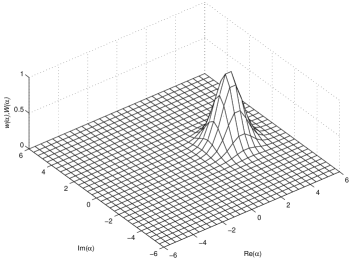
Figure 1: Surface plot of the initial distributions $W\left(\alpha,0\right)$ and $w\left(\alpha,0\right)$. In the quantum case, this distribution corresponds to an initial coherent state $\lvert\alpha_{0}\rangle\langle\alpha_{0}\rvert$ with $\alpha_{0}=3$, whereas in the classical case it corresponds to a gaussian distribution centered in $\alpha=3$ with unitary variance.

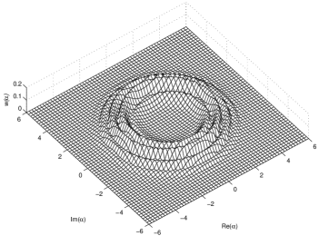
Figure 2: Surface plot of the classical distribution function for the anharmonic oscillator at $t=\pi\left(2g\right)^{-1}$ corresponding to the hamiltonian evolution ($\kappa=0$) of the initial condition shown in Fig. 1. For this case, $g/\omega=0.1$. Note the fine-structure yielded by the continuous spiraling of the distribution around the origin of the phase space.

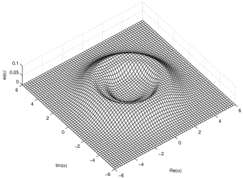
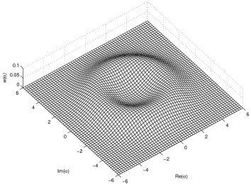
Figure 3: Surface plot of the classical distribution functions for the anharmonic oscillator at instants $t=\pi\left(2g\right)^{-1}$ (top) and $t=\pi g^{-1}$ (bottom) corresponding to the diffusive evolution ($\kappa/g=0.1$) of the initial condition shown in Fig. 1. For this case, $g/\omega=0.1$. Note that the fine-structure that should be yielded in the diffusionless regime (see Fig. 2) is gradually destroyed.

In the quantum version of the model, the unitary evolution of the Wigner function exhibits a very different behavior that the classical one. For times equal to $m\pi/\left(2g\right)$, where $m$ is an integer, the nonlinearity leads to the quantum superpositions of states ($m$ is odd) or revivals and anti-revivals ($m$ is even). These effects were already reported by Yurke and Stoler [7] and examples of them are given in Figs. 4 and 5.

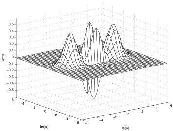
Figure 4: Surface plot of the Wigner function for the quantum anharmonic oscillator at $t=\pi\left(2g\right)^{-1}$ corresponding to the unitary evolution ($\kappa=0$) of the initial condition shown in Fig. 1. For this case, $g/\omega=0.1$. Note that the appearance of phase space interference due to the coherent superposition of states (Schrödinger cat state). At this time, the state exhibits some squeezing as well [10]. Compare with the corresponding classical one shown in Fig. 2.

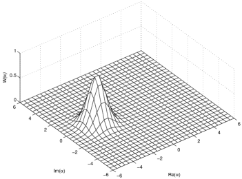
Figure 5: Surface plot of the Wigner function for the quantum anharmonic oscillator at $t=\pi g^{-1}$ corresponding to the unitary evolution ($\kappa=0$) of the initial condition shown in Fig. 1. For this case, $g/\omega=0.1$. At this instant, the oscillator exhibits an anti-revival since it is found in a coherent state with amplitude $-\alpha_{0}$, where $\alpha_{0}$ is the amplitude of the initial coherent state.

When the diffusion is included, the quantum effects discussed above are gradually suppressed. The interference in phase space is reduced, and the regions where the Wigner function is negative diminish (see Fig. 6). For later times, the Wigner function and the classical distribution take a form of an annular volume around the origin of the phase space. The annular region grows with time but its maximum value diminishes in order to mantain constant the integral of $W\left(\alpha,t\right)$ or $w\left(\alpha,t\right)$ over the phase space. This suggests that the Wigner function of the quantum diffusive AHO converges gradually to the corresponding classical distribution function. Non-unitary effects due to quantum dynamics of the open AHO were investigated by Milburn and Holmes [9], and by Daniel and Milburn [10], considering the coupling to a null and non-null temperature reservoir, respectively. In both works, the authors evaluates the time evolution of the Husimi function ($Q$ function), another phase space representation of the density operator. Their results show a similar behavior for the $Q$ function, in qualitative agreement with the one reported here.

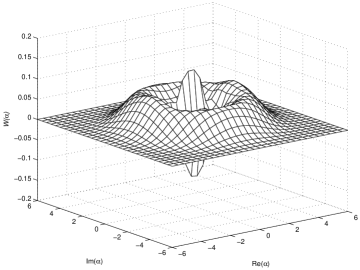
Figure 6: Surface plot of the Wigner function for the quantum anharmonic oscillator at instants $t=\pi\left(2g\right)^{-1}$ (top) and $t=\pi g^{-1}$ (bottom) corresponding to the diffusive evolution ($\kappa/g=0.1$) of the initial condition shown in Fig. 1. For this case, $g/\omega=0.1$. Comparing with Figs. 4 and 5 one notes that the phase space interferences and the revivals are gradually suppressed.

These results serve to illustrate the procedure and to show that the results are physically consistent. However, a detailed study of the quantum to classical transition in the AHO must take into account the role played by the parameters of interest, namely the nonlinearity strengh, the diffusion constant, and the amplitude of the initial coherent state (a measure of classicallity of the initial state). This work is in progress.

References

• [1] M. Brune et al., Phys. Rev. Lett. 77, 4887-4890 (1996).
• [2] M. A. Nielsen, and I. L. Chuang, Quantum Computation and Quantum Information (Cambridge: Cambridge University Press, 2000).
• [3] N. Gisin, G. Ribordy, W. Titel, and H. Zbinden, Rev. Mod. Phys. 77, 145-195 (2002).
• [4] D. Giulini et al., Decoherence and the Appearence of a Classical World in Quantum Theory (Berlin: Springer, 1996).
• [5] S. Habib, K. Shizume, and W. H. Zurek, Phys. Rev. Lett. 80, 4361-4365 (1998).
• [6] N. Wiebe, and L. E. Ballentine, e-print arXiv:quant-ph/0503170v1.
• [7] B. Yurke, and D. Stoler, Phys. Rev. Lett. 57, 13-16 (1986).
• [8] G. J. Milburn, Phys. Rev. A 33, 674-685 (1986).
• [9] G. J. Milburn, and C. A. Holmes, Phys. Rev. Lett. 56, 2237-2240 (1986).
• [10] D. J. Daniel, and G. J. Milburn, Phys. Rev. A 39, 4628-4640 (1989).
• [11] V. Pe$\check{\mathrm{r}}$inová, and A. Luk$\check{\mathrm{s}}$, Phys. Rev. A 41, 414-420 (1990).
• [12] S. Chaturvedi, and V. Srinivasan, Phys. Rev. A 43, 4054-4057 (1991).
• [13] K. V. Kheruntsyan, J. Opt. B: Quantum Semiclass. Opt. 1, 225-233 (1999).
• [14] G. P. Berman, A. R. Bishop, F. Borgonovi, and D. A. R. Dalvit, Phys. Rev. A 69, 062110 (2004).
• [15] M. Greiner, O. Mandel, T. W. Hänsch, and I. Bloch, Nature (London) 419, 51-54 (2002).
• [16] K. Kumar, J. Math. Phys. 6, 1928-1934 (1965).
• [17] R. M. Wilcox, J. Math. Phys. 8, 962-982 (1967).
• [18] R. Gilmore, J. Math. Phys. 15, 2090-2092 (1974).
• [19] W. Witschel, Int. J. Quantum Chem. 20, 1233-1241 (1981).
• [20] A. C. Oliveira, J. G. Peixoto de Faria, and M. C. Nemes, Phys. Rev. E 73, 046207 (2006).
• [21] F. Toscano, R. L. de Matos Filho, and L. Davidovich, Phys. Rev. A 71, 010101 (2005).
• [22] S. J. Wang, M. C. Nemes, A. N. Salgueiro, and H. A. Weidenmüller, Phys. Rev. A 66, 033608 (2002).
• [23] A. Royer, Phys. Rev. A 43, 44-56 (1991).
• [24] K. Wódkiewicz, and J. H. Eberly, J. Opt. Soc. Am. B 2, 458-466 (1985).
• [25] G. Dattoli, M. Richetta, and A. Torre, Phys. Rev. A 37, 2007-2011 (1988).
• [26] E. P. Wigner, Phys. Rev. 40, 749-759 (1932).
• [27] M. Hillery, R. F. O’Connel, M. O. Scully, and E. P. Wigner, Phys. Rep. 106, 121-167 (1984).
• [28] H.-W. Lee, Phys. Rep. 259, 147-211 (1995).
• [29] S. Steinberg, in Lie Methods in Physics, ed. J. S. Mondragón, and K. B. Wolf, Lecture Notes in Physics 250 (Berlin: Springer, 1985).
• [30] A. M. Perelomov, Generalized Coherent States and their Applications (Berlin: Springer, 1986).
• [31] J. J. Sakurai, Modern Quantum Mechanics (Reading, MA: Addison-Wesley, 1994).
• [32] M. A. Marchiolli, Rev. Bras. Ens. Fís. 24, 421-36 (2002).
• [33] I. S. Gradshteyn, and I. M. Ryzhik, Table of Integrals, Series and Products (San Diego: Academic Press, 1980).