Macroscopic entanglement by entanglement swapping

Abstract

We present a scheme for entangling two micromechanical oscillators. The scheme exploits the quantum effects of radiation pressure and it is based on a novel application of entanglement swapping, where standard optical measurements are used to generate purely mechanical entanglement. The scheme is presented by first solving the general problem of entanglement swapping between arbitrary bipartite Gaussian states, for which simple input-output formulas are provided.

Micromechanical resonators with fundamental vibrational mode frequencies in the range 10 MHz–1 GHz can now be fabricated Roukes03 . Applications include fast, ultrasensitive displacement detectors cleland03 , electrometers, and radio frequency signal processors. Advances in the development of micromechanical devices also raise the fundamental question of whether mechanical systems containing macroscopic numbers of atoms will exhibit quantum behavior. In particular, it is interesting to see under which conditions it is feasible to prepare micromechanical oscillators in entangled states, where the quantum nature becomes most manifest. Proposals of this kind recently appeared in the literature. One could entangle a nanomechanical oscillator with a Cooper-pair box Armour03 , with an ion zoller , or with single photons Marshall03 ; moreover Ref. eisert studied how to entangle an array of nanomechanical oscillators, Ref. CRITERIO proposed to entangle two mirrors of an optical ring cavity, while Ref. Peng03 considered two mirrors of two different cavities illuminated with entangled light beams. In this Letter we will show how to entangle two micromechanical oscillators, which are parts of two different micro-opto-mechanical systems, by means of continuous variable (CV) entanglement swapping performed on the “optical parts”. Our proposal exploits some results of Ref. PRLePRA , which showed how radiation pressure can entangle a vibrational mode of a mirror with the back-scattered sideband modes of an intense optical beam. Thanks to this optomechanical entanglement, one can entangle two different mechanical oscillators by performing appropriate optical measurements. Note that, very recently, Ref. Carmon05 has experimentally observed the two considered sideband modes, although no measurements of entanglement have been performed. The proposal is presented by first solving the general problem of CV entanglement swapping between arbitrary Gaussian bipartite states, for which we are able to derive compact input-output formulas. Such a study suitably generalizes the previous fully optical theoretical analyses vanloock and it has a straightforward application to our physical scheme.

Let us first study entanglement swapping with Gaussian states in general. We consider a pair of CV systems labelled by $k=1,2$, where each of them is described by a pair of conjugate dimensionless quadratures $\hat{x}_{k}$ and $\hat{p}_{k}$. Introducing the vector $\hat{\xi}^{T}\equiv(\hat{x}_{1},\hat{p}_{1},\hat{x}_{2},\hat{p}_{2})$, we can write the canonical commutation relations in the compact form $[\hat{\xi}_{l},\hat{\xi}_{m}]=i\mathcal{J}_{lm}$ ($l,m=1,...,4$), where

$$\mathcal{J}\equiv J\oplus J,~{}J\equiv\left(\begin{array}[]{cc}0&1\\ -1&0\end{array}\right)\text{ ,}$$ (1)

and $\oplus$ denotes the usual direct sum operation. An arbitrary state $\rho_{12}$ of the two oscillators can be described by its Wigner characteristic function $\Phi_{12}(\vec{\zeta})\equiv\mathrm{Tr}[\rho_{12}\hat{D}(\vec{\zeta})]$, where $\hat{D}(\vec{\zeta})=\exp(-i\hat{\xi}^{T}\vec{\zeta})$ is the Weyl operator and $\vec{\zeta}\in\mathbb{R}^{4}$. Such a state is said to be Gaussian if the corresponding characteristic function is Gaussian, i.e., $\Phi_{12}(\vec{\zeta})=\exp(-\vec{\zeta}^{T}V\vec{\zeta}/2+i\vec{d}^{T}\vec{\zeta})$. In such a case, the state $\rho_{12}$ is fully characterized by its displacement $\vec{d}\equiv\langle\hat{\xi}\rangle$ and its correlation matrix (CM) $V$, whose generic element is defined as $V_{lm}\equiv\langle\Delta\hat{\xi}_{l}\Delta\hat{\xi}_{m}+\Delta\hat{\xi}_{m}\Delta\hat{\xi}_{l}\rangle/2$ where $\Delta\hat{\xi}_{l}\equiv\hat{\xi}_{l}-\langle\hat{\xi}_{l}\rangle$. All the information about the quantum correlations between the two oscillators is contained in the CM, which is a $4\times 4$, real and symmetric matrix, satisfying the uncertainty principle $V+i\mathcal{J}/2\geq 0$. Putting the CM into the form

$$V\equiv\left(\begin{array}[]{cc}A&D\\ D^{T}&C\end{array}\right)\text{ ,}$$ (2)

where $A,C,$ and $D$ are $2\times 2$ real matrices, one can easily derive a quantitative measure of entanglement. In fact, from the CM (2), one can compute the two quantities

$$\eta^{\pm}\equiv 2^{-1/2}\left[\Sigma(V)\pm\left(\Sigma(V)^{2}-4\det V\right)^{1/2}\right]^{1/2}\text{ ,}$$ (3)

where $\Sigma(V)\equiv\det A+\det C-2\det D$. Such quantities correspond to the symplectic eigenvalues Salerno1 of the matrix $\Lambda_{b}V\Lambda_{b}$, which is obtained from $V$ through the partial transposition (PT) transformation $\Lambda_{b}\equiv\mathrm{\Delta}[1,1,1,-1]$, where $\mathrm{\Delta}[\lambda_{1},...,\lambda_{n}]$ denotes a diagonal matrix with the $n$ entries $\lambda_{k}$ in the diagonal. One can then prove Salerno1 that the minimum PT symplectic eigenvalue $\eta^{-}$ represents an entanglement monotone, since it is connected to the logarithmic negativity by

$$E_{\mathcal{N}}=\max[0,-\ln 2\eta^{-}]\text{ .}$$ (4)

In particular, the Gaussian state $\rho_{12}$ is entangled if and only if $\eta^{-}<1/2$, which is equivalent to $E_{\mathcal{N}}>0$ according to Eq. (4).

In general, CV entanglement swapping involves two pairs of modes, $(a,c_{1})$, owned by Alice and Charlie, and $(b,c_{2})$, owned by Bob and Charlie. We assume that the two pairs are described by two arbitrary Gaussian states $\rho_{ac}$ and $\rho_{bc}$, having generic CMs

$$V_{ac}=\left(\begin{array}[]{cc}A&D_{1}\\ D_{1}^{T}&C_{1}\end{array}\right),\text{ }V_{bc}=\left(\begin{array}[]{cc}B&D_{2}\\ D_{2}^{T}&C_{2}\end{array}\right)\text{ ,}$$ (5)

where $A,B,C_{1},C_{2},D_{1},D_{2}$ are $2\times 2$ real matrices. The basic idea of entanglement swapping is to transfer the bipartite entanglement within the near pairs Alice-Charlie and Charlie-Bob to the distant pair Alice-Bob, by means of a suitable local operation and classical communication performed by Charlie. In fact, Charlie mixes his two modes $c_{1}$ and $c_{2}$ through a balanced beam splitter (BS) and then he measures the output quadratures $\hat{x}_{c_{2}}-\hat{x}_{c_{1}}$ and $\hat{p}_{c_{2}}+\hat{p}_{c_{1}}$. After this measurement, which realizes a CV version of a Bell measurement, he communicates the outcomes to Alice and Bob vanloock . The final output state $\rho_{ab}$ of Alice and Bob turns out to be a Gaussian state whose CM can be expressed in terms of the input matrices’ blocks as

$$V_{ab} =V_{ab}^{tr}-g\left(\begin{array}[]{cc}D_{1}&\\ &D_{2}\end{array}\right)\mathcal{J}\left[\Lambda_{b}\left(\begin{array}[]{cc}C_{1}&C_{1}\\ C_{1}&C_{1}\end{array}\right)\Lambda_{b}\right.$$ (10)

$$\left.~{}~{}~{}~{}~{}~{}~{}~{}+\Lambda_{a}\left(\begin{array}[]{cc}C_{2}&C_{2}\\ C_{2}&C_{2}\end{array}\right)\Lambda_{a}\right]\mathcal{J}^{T}\left(\begin{array}[]{cc}D_{1}^{T}&\\ &D_{2}^{T}\end{array}\right)\text{ ,}$$ (15)

where $V_{ab}^{tr}\equiv A\oplus B$, $\Lambda_{a}\equiv R\oplus I$ and $\Lambda_{b}\equiv I\oplus R$ are the PT transformations over Alice and Bob respectively, with $R=\mathrm{\Delta}[1,-1]$ and $I=\mathrm{\Delta}[1,1]$, and finally $g^{-1}=\det C_{1}+\det C_{2}+\mathrm{Tr}(RC_{2}RJC_{1}J^{T})$. The general result of Eq. (15) specializes to a very simple form if the input matrices $V_{ab}$ and $V_{bc}$ are put in the normal form, i.e., $A=aI,$ $B=bI,$ $C_{k}=c_{k}I$ and $D_{k}=\mathrm{\Delta}[d_{k},d_{k}^{\prime}]$ for $k=1,2$. This can always be achieved by means of local symplectic transformations DuanPRL at Alice, Bob and Charlie’s sites, which therefore do not affect the entanglement resources of the initial states $\rho_{ac}$ and $\rho_{bc}$. In such a case, we have

$$V_{ab} = \left(\begin{array}[]{cc}aI&\\ &bI\end{array}\right)-\frac{1}{c_{1}+c_{2}}\times$$ (21)

$$\left(\begin{array}[]{cc}\mathrm{\Delta}[d_{1}^{2},d_{1}^{\prime 2}]&\mathrm{\Delta}[-d_{1}d_{2},d_{1}^{\prime}d_{2}^{\prime}]\\ \mathrm{\Delta}[-d_{1}d_{2},d_{1}^{\prime}d_{2}^{\prime}]&\mathrm{\Delta}[d_{2}^{2},d_{2}^{\prime 2}]\end{array}\right)\text{ ,}$$

providing a straightforward expression for the CM of the final Alice and Bob’s state.

In general, the output entanglement cannot be expressed as a simple function of the input entanglement. Nonetheless, this becomes possible in the symmetrical case of identical physical resources shared by the two pairs, i.e., when $\rho_{ac}=\rho_{bc}\equiv\rho_{in}$. If the input matrix $V_{in}$ of $\rho_{in}$ is converted from the general form of Eq. (2) to its normal form, the transformation connecting $V_{in}$ to the output matrix $V_{out}$ of $\rho_{out}\equiv\rho_{ab}$ can be written as

$$V_{in} \equiv \left(\begin{array}[]{cc}aI&\mathrm{\Delta}[d,d^{\prime}]\\ \mathrm{\Delta}[d,d^{\prime}]&cI\end{array}\right)\longrightarrow V_{out}=\frac{1}{2c}\times$$ (27)

$$\left(\begin{array}[]{cc}\mathrm{\Delta}[2ac-d^{2},2ac-d^{\prime 2}]&\mathrm{\Delta}[d^{2},-d^{{}^{\prime}2}]\\ \mathrm{\Delta}[d^{2},-d^{{}^{\prime}2}]&\mathrm{\Delta}[2ac-d^{2},2ac-d^{\prime 2}]\end{array}\right)\text{.}$$

Note that in Eq. (27) the output state is a symmetric Gaussian state, whose entanglement properties have been widely studied in literature Cirac . By applying Eq. (3) to $V_{in}$ and $V_{out}$, one can connect the PT symplectic eigenvalues $\eta_{out}^{\pm}$ of the output matrix with the ones $\eta_{in}^{\pm}$ of the input matrix by the simple input-output relations

$$\eta_{out}^{-} =c^{-1}\eta_{in}^{+}\eta_{in}^{-}=c^{-1}\sqrt{\det V_{in}}\text{ ,}$$ (28)

$$\eta_{out}^{+} =a\text{ .}$$ (29)

Note that the output eigenvalues are uniquely determined by the local symplectic invariants of the original CM of Eq. (2), since here $a=\sqrt{\det A}$ and $c=\sqrt{\det C}$.

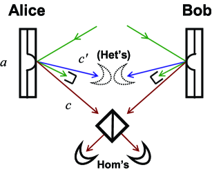
Figure 1: Two identical intense laser pulses are incident on two identical micromechanical oscillators. Each beam excites a vibrational mode, which generates two optical sideband modes in the back-scattered field. Both reflected Stokes modes are mixed through a balanced BS and the output ports are homodyned. The anti-Stokes modes can be either ignored (non-assisted strategy) or heterodyned (assisted strategy).

Let us now apply the above results and, in particular, the input-output relation of Eq. (28), to see how one can entangle two micromechanical oscillators by means of entanglement swapping. Consider the system of Ref. PRLePRA , which is schematically depicted in the left part of Fig. 1. The radiation pressure of an intense monochromatic laser beam (frequency $\omega$), incident on a micromechanical oscillator, generates an effective coupling between a vibrational mode of the oscillator (label $a$, frequency $\Omega$) and the two first optical sideband modes induced by the vibrations in the back-scattered field, i.e., the Stokes mode (label $c$, frequency $\omega-\Omega$) and the anti-Stokes mode (label $c^{\prime}$, frequency $\omega+\Omega$) (e.g., see Ref. Carmon05 , where these sidebands have been generated and detected). The vibrational mode is characterized by a relaxation time $\Gamma^{-1}$ which globally takes into account several damping effects, like internal losses of the medium and those due to the clamping. All these damping effects can be neglected if the duration of the laser pulse is much shorter than $\Gamma^{-1}$ so that the system dynamics can be assumed unitary during the interaction time. In this unitary description of the process, the interaction Hamiltonian for the vibrational mode, the Stokes mode and the anti-Stokes mode is given by ${\hat{H}}=-i\hbar\chi(\hat{a}\hat{c}-\hat{a}^{{\dagger}}\hat{c}^{{\dagger}})-i\hbar\theta(\hat{a}^{{\dagger}}\hat{c}^{\prime}-\hat{a}\hat{c}^{\prime{\dagger}})$, where $\chi$ and $\theta$ are coupling constants whose ratio $r\equiv\theta/\chi=\left[(\omega+\Omega)/(\omega-\Omega)\right]^{1/2}\geq 1$ depends only on the involved frequencies, and the operators $\hat{a}$, $\hat{c}$ and $\hat{c}^{\prime}$ are the annihilation operators of the three modes $a$, $c$ and $c^{\prime}$, satisfying $\left[\hat{a},\hat{a}^{\dagger}\right]=\left[\hat{c},\hat{c}^{\dagger}\right]=1$, etcetera. Starting from vacuum states for the optical modes and a thermal state for the vibrational mode, with mean excitation number $\bar{n}=[\exp(\hbar\Omega/KT)-1]^{-1}$ ($T$ being the temperature), the evolved state is Gaussian with the $6\times 6$ CM

$$V_{cac^{\prime}}=\left(\begin{array}[]{ccc}(\mathcal{A}+1/2)I&\mathcal{C}R&\mathcal{F}R\\ \mathcal{C}R&(\mathcal{B}+1/2)I&-\mathcal{D}I\\ \mathcal{F}R&-\mathcal{D}I&(\mathcal{E}+1/2)I\end{array}\right)\text{ ,}$$ (30)

where $\mathcal{A}$, $\mathcal{B}$, $\mathcal{C}$, $\mathcal{D}$, $\mathcal{E}$ and $\mathcal{F}$, explicitly given in Ref. PRLePRA , depend on $r$, $\bar{n}$ and the scaled time $t^{\prime}\equiv t(\theta^{2}-\chi^{2})^{1/2}$.

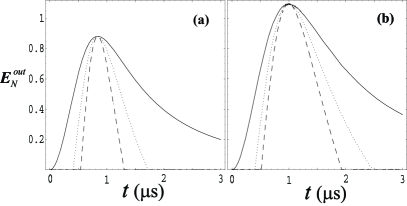
Figure 2: Output log-negativity $E_{\mathcal{N}}^{out}$ versus time $t$, for $T=0$K (solid), $T=5$mK (dotted), $T=300$K (dashed) (see text for the other parameters). (a) refers to the non-assisted strategy; (b) refers to the assisted strategy.

Suppose that Alice and Bob are supplied with two identical micromechanical oscillators, equally illuminated by an intense laser pulse, and suppose that the reflected Stokes and anti-Stokes modes are sent to Charlie (i.e., to our experimental detection apparatus). In a first strategy (see Fig. 1), Charlie simply traces out the anti-Stokes modes and performs a CV Bell measurement over the remaining Stokes modes. In such a case, just after reading out the measurement results at time $t$, the two mechanical oscillators are described by a Gaussian state $\rho_{out}$ with CM $V_{out}$ given in Eq. (27) through the replacements: $a=\mathcal{B}+1/2,$ $c=\mathcal{A}+1/2$ and $d=-d^{\prime}=\mathcal{C}$. By applying Eq. (28), one can compute the entanglement $\eta_{out}^{-}$ of the output state. Adopting the parameters $(\theta^{2}-\chi^{2})^{1/2}\simeq 10^{3}$ s^-1, $r=1+2.5\times 10^{-7}$ and $\Omega=5\times 10^{8}$ s^-1, we have studied the output log-negativity $E_{\mathcal{N}}^{out}=\max[0,-\ln 2\eta_{out}^{-}]$ as a function of the interaction time $t$, and for different values of the external temperature $T$. In Fig. 2(a) one can see the existence of wide non-zero time regions giving a strong entanglement between the two mechanical modes, even for large temperatures. For instance, if the Bell measurement is performed after an interaction time $t\sim 0.8\mu$s, one gets an optimal entanglement measure $E_{\mathcal{N}}^{out}\sim 0.88$, which does not depend on temperature (see the maximum in Fig. 2(a)). This is an effect of the quantum interference which holds provided that the mechanical damping time $\Gamma^{-1}$ is much longer than the duration of the laser pulse and therefore the unitary treatment of the process is valid. However, the living time of the generated entanglement will depend on the damping time $\Gamma^{-1}$ scaled by a factor depending on temperature. This decoherence time is given by $\gamma^{-1}=\Gamma^{-1}\ln[(2\bar{n}+1-2\eta_{out}^{-})(2\bar{n}+e^{-1}-2e^{-1}\eta_{out}^{-})^{-1}]$, which gives the limits $\gamma^{-1}\simeq 1/\Gamma$ for $T\longrightarrow 0$ and $\gamma^{-1}\simeq\hbar\Omega(2\Gamma KT)^{-1}$ for $KT\gg\hbar\Omega$. Therefore, even for long $\Gamma^{-1}$, the entanglement living time will be affected by temperature and it will be very short for high temperatures. For instance, if $\Omega\simeq 5\times 10^{8}$ s^-1 and $\Gamma^{-1}\simeq 1$s, one has $\gamma^{-1}\simeq 3$ $\mu$s at $T\simeq 300$ K, which has to be compared with $\gamma^{-1}\simeq 1$ ms at $T\simeq 1$ K. It is therefore necessary to consider low temperatures in order to preserve the mechanical entanglement, even if this assumption is not crucial for its generation. Now, since the effective masses of the vibrational modes can be of the order of $10^{-10}$ kg, this result proves the feasibility of entangling massive macroscopic objects combining radiation pressure effects and simple optical homodyne measurements. Actually, this performance can be further improved by assisting the Bell measurement on the Stokes modes by additional heterodyne measurements on the anti-Stokes modes (see Fig. 1). In fact, heterodyne measurements are the Gaussian conditional measurements optimizing the entanglement between the oscillator and the Stokes mode optim . Adopting this modified protocol, the output state $\rho_{out}$ will be again Gaussian, but with a modified CM $V_{out}$, as given by Eq. (27) with the replacements: $a=\mathcal{B}+1/2-\mathcal{D}^{2}/(\mathcal{E}+1),$ $c=\mathcal{A}+1/2-\mathcal{F}^{2}/(\mathcal{E}+1)$ and $d=-d^{\prime}=\mathcal{C}+\mathcal{D}\mathcal{F}/(\mathcal{E}+1)$. The improvement is shown in Fig. 2(b) where the entanglement time regions are wider and the maximum achievable entanglement is larger than before ($E_{\mathcal{N}}^{out}\sim 1.1$ at $t\sim 1\mu$s).

An important related issue is the experimental detection of the generated macroscopic entanglement. In general, proving the existence of entanglement between two oscillators requires the measurement of two different linear combinations of quadratures, like the relative distance $\hat{X}_{rel}\equiv\hat{x}_{a}-\hat{x}_{b}$ and the total momentum $\hat{P}_{tot}\equiv\hat{p}_{a}+\hat{p}_{b}$ CRITERIO ; DuanPRL . However, in the present case, the final Gaussian state of Alice and Bob, both in the assisted and non-assisted case, is a symmetrical channel where the variance of relative distance and total momentum are equal, i.e., $\langle(\Delta\hat{X}_{rel})^{2}\rangle=\langle(\Delta\hat{P}_{tot})^{2}\rangle$ (from Eq. (27) with $d=-d^{\prime}$), and, in particular, $\langle(\Delta\hat{X}_{rel})^{2}\rangle=2\eta_{out}^{-}$ (from Eq. (28)). If the two micromechanical oscillators are highly reflecting mirrors, they can be used as end mirrors of a Fabry-Perot cavity. It is known that when this cavity is resonantly driven by an intense laser field, the detection of the phase quadrature of the cavity output provides a real-time quantum non-demolition measurement of the mirror relative distance $\hat{X}_{rel}$ qnd . Thus, if the cavity is driven soon after Charlie’s measurements and one performs a homodyne detection of the output field, one can measure the variance $\langle(\Delta\hat{X}_{rel})^{2}\rangle$ and, therefore, the log-negativity of the swapped state via Eq. (4). If the two oscillators are different, the final state of Alice and Bob is no more symmetrical and one has to measure both $\langle(\Delta\hat{X}_{rel})^{2}\rangle$ and $\langle(\Delta\hat{P}_{tot})^{2}\rangle$ in order to surely detect entanglement (e.g., see Ref. pinard ). Alternatively one can measure $\hat{x}$ and $\hat{p}$ of each oscillator by shining a second, intense “reading” laser pulse on it, and exploiting again the same optomechanical scattering process. In fact, as shown in Ref. PRLePRA , by performing a heterodyne measurement of the linear combination of the two sidebands $c-c^{\prime\dagger}$, one can reconstruct the oscillators’ state. Therefore one can detect the generated mechanical entanglement provided that the living time of the entanglement, $\gamma^{-1}$, is long enough and this is achievable at cryogenic temperatures. In fact, as we have seen above, the thermal environment makes the mechanical entanglement decay with a relaxation time which can be quite long at low enough $T$ ($\gamma^{-1}\simeq 1$ ms at $T\simeq 1$ K if $\Omega\simeq 5\times 10^{8}$ s^-1 and $\Gamma^{-1}\simeq 1$s).

In conclusion, we have presented a scheme for entangling two micromechanical oscillators by entanglement swapping. The scheme exploits the optomechanical entanglement between each oscillator and the reflected sideband modes of an intense laser field, which can be generated by radiation pressure. Optical measurements are then able to swap this entanglement to the oscillators, with the non-trivial effect of changing the entanglement from optomechanical to purely mechanical. To study the scheme, we have first solved the general problem of entanglement swapping between generic bipartite Gaussian states, providing simple input-output formulas.

This work has been supported by MIUR (PRIN-2003): “Schemes for exploiting entanglement in optomechanical devices” and by the European Commission through FP6/2002/IST/FETPI SCALA: “Scalable Quantum computing with Light and Atoms”, Contract No. 015714.

References

- (1) X. M. H. Huang et al., Nature (London) 421, 496 (2003).
- (2) R. G. Knobel and A. N. Cleland, Nature (London) 424, 291 (2003); M. D. LaHaye et al., Science 304, 74 (2004).
- (3) A. D. Armour et al., Phys. Rev. Lett. 88, 148301 (2002).
- (4) L. Tian and P. Zoller, Phys. Rev. Lett. 93, 266403 (2004).
- (5) W. Marshall et al., Phys. Rev. Lett. 91, 130401 (2003);
- (6) J. Eisert et al., Phys. Rev. Lett. 93, 190402 (2004).
- (7) S. Mancini et al., Phys. Rev. Lett. 88, 120401 (2002).
- (8) J. Zhang et al., Phys. Rev. A 68, 013808 (2003).
- (9) S. Mancini et al., Phys. Rev. Lett. 90, 137901 (2003); S. Pirandola et al., Phys. Rev. A 68, 062317 (2003).
- (10) T. Carmon et al., Phys. Rev. Lett. 94, 223902 (2005).
- (11) P. Van Loock and S. L. Braunstein, Phys. Rev. A, 61, 010302(R) (2000).
- (12) G. Adesso et al., Phys. Rev. A 70, 022318 (2004).
- (13) L.-M. Duan et al., Phys. Rev. Lett. 84, 2722 (2000).
- (14) G. Giedke et al., Phys. Rev. Lett. 91, 107901 (2003); M. M. Wolf et al., Phys. Rev. A 69, 052320 (2004); M. M. Wolf et al., Phys. Rev. Lett. 92, 087903 (2004).
- (15) S. Pirandola et al., Phys. Rev. A 71, 042326 (2005).
- (16) K. Jacobs et al., Phys. Rev. A 49, 1961 (1994).
- (17) M. Pinard et al., Europhys. Lett. 72, 747 (2005).