Array of planar Penning traps as a nuclear magnetic resonance molecule for quantum computation

Abstract

An array of planar Penning traps, holding single electrons, can realize an artificial molecule suitable for NMR-like quantum information processing. The effective spin-spin coupling is accomplished by applying a magnetic field gradient, combined to the Coulomb interaction acting between the charged particles. The system lends itself to scalability, since the same substrate can easily accomodate an arbitrary number of traps. Moreover, the coupling strength is tunable and under experimental control. Our theoretical predictions take into account a realistic setting, within the reach of current technology.

I Introduction

In this proposal we bring together the best of two avenues to quantum information processing: nuclear magnetic resonance (NMR) jones and ion trapping leibfried1 . Both approaches have provided the first experimental demonstrations of fundamental quantum logic gates and quantum algorithms, though still limited to few qubits. Actually, it is relatively simple to build a small NMR quantum computer, useful for a proof-of-principle test of quantum algorithms, but unable to perform any real computation, involving hundreds of qubits. Indeed, the scalability seems to be a rather tough question for NMR quantum computing. Another disadvantage of NMR quantum computation is that NMR experiments deal with a large number of molecules, building up an ensemble of indistinguishable quantum computers. This fact brings in relevant theoretical and practical implications: from the system initialisation to the debate on the same quantum character of the computation carried out with such a device. However, NMR techniques, based on radio frequency (rf) and microwave (mw) pulses, enable to carefully prepare, manipulate, and detect the qubit states with relative ease. Spatial separation of the qubits is not required, since different qubits are distinguished using different resonance frequencies.

On the other hand, in ion trap quantum computation, qubits are stored in isolated quantum systems, arranged to form strings of trapped particles, spatially separated and singly addressable with optical radiation rainerblatt ; Leibfried . Such systems can be prepared in their motional ground state via sophisticated laser cooling techniques. Coherent manipulation of the qubits requires strongly focused pulses of controlled intensity, phase and duration at optical frequencies. The required setup is rather involved and the experimental realization challenging. These technical problems have motivated other proposals by Wunderlich et al. to implement a quantum computer, based on trapped ions in a linear Paul trap, but using long-wavelength radiation, in the radio frequency or microwave range mintert . To this end, internal and external degrees of freedom of the trapped ion are coupled by means of a magnetic field gradient. Moreover, in a linear Paul trap, the collective vibrational modes of a chain of $N$ two-level ions extend this coupling to different ions. The system is formally analogous to a collection of spins, interacting through the so-called $J$-coupling, typical of nuclear spins in molecules wunderlich_1 ; wunderlich_2 ; wunderlich_3 . However, the proposal by Wunderlich et al. presents some drawbacks, especially for the scalability, due to the fact that all the ions are stored in the same linear trap. A more flexible design would be based on a string of individually tailored microtraps, each of them trapping a single ion mchugh . These ideas are versatile and can be adapted to other scenarios.

Our system consists of an array of Penning traps, each of them confining a single electron. A Penning trap makes use of static electric and magnetic fields to trap charged particles, like ions or electrons. In particular, the magnetic field provides the radial confinement, which, in a Paul trap, is achieved by means of an oscillating (radio frequency) electric field. The resulting dynamics of a particle in a Paul trap is harmonic in all directions, whereas in a Penning trap the combination of the electric and magnetic fields gives rise to a more complicated orbital motion, which is the superposition of the magnetron and cyclotron oscillators. These differences should be taken into account, when describing the effects of an additional magnetic gradient on the trapped particle dynamics.

We choose to trap electrons instead of ions, because of their smaller mass, which results in higher trapping frequency for the quantized external degrees of freedom. Indeed, the typical resonance frequencies of the resulting electron motion lie in the radiofrequency and microwave domain, making it possible to employ the same technological resources and methods developed for NMR experiments. Moreover, differently from a Paul trap, a Penning trap does not rely on rf fields, a benefit in terms of stability of the trapping potential. In turns, this translates into less decoherence affecting the trapped particles. Therefore, electrons trapped in vacuum seem to be a promising candidate for quantum information processing ciaramicoli4 ; ciaramicoli_5 , taking advantage of the techniques and strategies devised both for NMR and ion trapping quantum computing.

What we have in mind is a new concept of planar Penning traps stahl , characterised by an open geometry. The trap electrodes are deposited on a ceramic substrate by means of well-established thin film or thick film technology, which allows for a variety of different configurations as well as dimensions. The trapping mechanism relies, as in conventional Penning traps, on the application of a magnetic field together with an electrostatic quadrupole potential. A single trapped electron is confined in vacuum at an adjustable distance from the trap surface. The same substrate can accomodate several traps in order to form a regular one or two dimensional array of trapped particles. Qubits are encoded in the natural two-level system provided by the electron spin in the external strong magnetic field, similarly to what happens for NMR spin one-half nuclei. The two possible spin orientations $|\uparrow\rangle$ and $|\downarrow\rangle$ represent, respectively, the logic states $|1\rangle$ and $|0\rangle$. Here, however, the two spin levels are greatly separated in energy and thermal excitation is completely negligible, especially at the trap cryogenic temperatures. Hence, the system, after initialisation, remains in its ground state, corresponding to the spin-down state. We have already observed that in order to make the spin qubits distinguishable, one has to introduce a small magnetic gradient ciaramicoli4 . Actually, with a judicious choice of the magnetic gradient, that in our configuration depends on all the spatial coordinates, we can also build up a molecule-like system. In the present geometry, the magnetic field gradient is applied across the substrate in order to differentiate among the spin resonance frequencies at each trapping site. Therefore, the spin qubits are distinguishable and can be selectively frequency addressed via microwave pulses. The same magnetic field gradient, mediated by the long range Coulomb interaction, enables the effective spin-spin coupling between different electrons. The resulting system may be regarded as an artificial molecule suitable for NMR quantum computation. Actually, we can even envisage applications to simulate other quantum systems, like the Ising model. Our system offers obvious advantages in terms of scalability. In addition, the spin-spin coupling depends on external parameters, like the strength of the magnetic field gradient, the trapping frequencies, and the trap separation, that can be adjusted to obtain the optimal performance of the quantum processor. We point out that this coupling is proportional to $1/d^{3}$, with $d$ being the inter-trap distance. Therefore, the spin-spin coupling strength is relevant only for nearest-neighbor electrons, while rapidly decays along the electron chain.

Finally, for what concerns the initialisation of the system, or, in other words, how to reset the quantum register to the state $|0\rangle$, several strategies could be followed. A possible one is to apply a transverse oscillating magnetic field resonant with the frequency difference between the cyclotron motion and the spin precession. When the magnetic gradient is off the transverse field will flip the spin up state of each particle transfering the energy to the corresponding cyclotron motion, which will release its energy to the environment via syncrotron radiation.

The manuscript is organized as follows. In Sec. II we describe the trap design and how to create a scalable device, putting several planar traps on the same substrate. The theoretical framework is developed in Sec. III, where we discuss the role of the applied magnetic field gradient to achieve the individual frequency addressability of the qubits (Sec. III.1) and derive an analytical expression for the effective spin-spin coupling (Sec. III.2). As an example we illustrate how to implement a set of fundamental quantum logic gates with the resulting NMR-like molecule, made out of trapped electrons (Sec. IV). The concluding remarks and the future perspectives for the system are summarized in Sec. V.

II The planar Penning trap

We have tried to design a trap which fulfills the needs of quantum computation and at the same time ensures the same amount of control and precision already achieved with conventional traps. To that end we consider a planar Penning trap, which is shown schematically in Fig. 1. The planar trap is a Penning trap in the sense that both electric and magnetic static fields are used to confine three-dimensionally a charged object. A generic Penning trap generates a quadrupolar static electric field together with a homogeneous and static magnetic field aligned in the direction of the symmetry axis, which we’ll assume to be $z$. The magnetic field confines a charged particle radially, whereas the electric field provides the confinement along the $z$ axis bossBook . Since the ideal quadrupole potential depends on the square of the coordinates, the motion in an ideal trap can be decomposed in three independent harmonic oscillators which are commonly denominated by cyclotron, magnetron and axial, each of them having different characteristic frequencies.

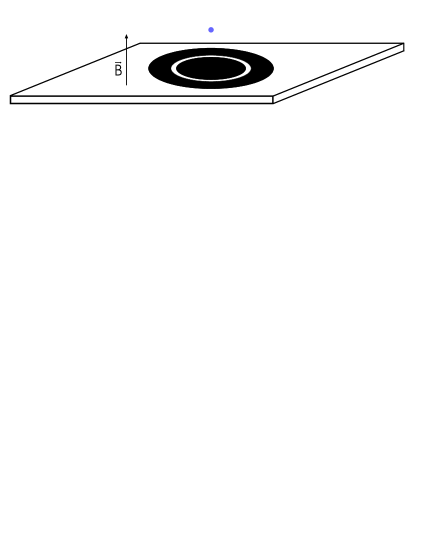
Figure 1: Simplest configuration of a planar trap with two electrodes (black) on an isolator substrate (white).

When the trap is not ideal, due to imperfectly homogeneous or quadrupolar fields, respectively, the three eigenmotions couple and can no longer be described as independent. However, the effects of such a coupling can be used for a number of applications, see e.g. pritchard ; Verdu ; Djekic .

II.1 General trap properties

A planar trap is a novel concept of trap stahl which allows for easy access with radiation, because of its open geometry, and lends itself to form a two dimensional array on the same substrate. In addition, it has the advantage that well-known methods to produce and miniaturize it are available.

As shown in Fig. 1, it consists of a collection of circular electrodes printed on an isolating substrate. The simplest planar structure has two different electrodes to which voltages of opposite sign are applied. The trap is lying on the $x-y$ plane and provides an electrostatic potential minimum along the $z$ axis at a distance $z_{0}$ from the substrate. A strong homogeneous static magnetic field of the order of few Tesla is aligned in the $z$ direction and provides radial confinement.

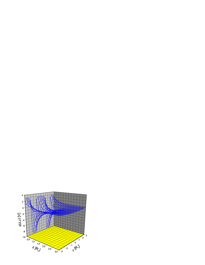
Figure 2: Electrostatic potential with three electrodes ($V_{1}=3V,V_{2}=-10V,V_{3}=3V$). One can see that the local potential minimum, in the $z$-direction around $\rho=0$, is almost quadrupolar even with the intrinsic asymmetry of the trap.

An example of 3D potential is shown in Fig. 2 for a configuration having three electrodes. The potential is obviously asymmetric and this implies that one needs to fine tune the applied voltages with more care than in a cylindrical trap. Another implication of its asymmetry is that one can move the position of the minimum along $z$. By varying the relative strength of the negative electrodes with respect to positive ones, a particle which is trapped around the minimum will vary its location under the control of the experimenter. This feature could be useful to study the problem of decoherence caused by a metallic plate, which depends on the distance of the particle from the plate patch .

The potential along the $z$ axis can, in the case of adjacent electrodes, be obtained analitically from a Bessel-Fourier series expansion and reads

$$\phi(z)=\sum_{i=1}^{N_{elec.}}V_{i}\left(\frac{z}{\sqrt{z^{2}+R_{i-1}^{2}}}-\frac{z}{\sqrt{z^{2}+R_{i}^{2}}}\right),$$ (1)

where $R_{i-1}$ is the inner radius of the $i$-th electrode ($R_{0}\equiv 0$, since the first electrode is a disc). $V_{i}$ is the voltage applied to electrode $i$ and $N_{elec.}$ is the number of electrodes stahl . The minimum of that function cannot be evaluated analitically, but it can be shown numerically that $z_{0}$, the minimum position, has a value of the order of $R_{1}$, the radius of the central electrode.

For electrons lying in the region near the trap axis, $\rho\ll R_{1}$, the potential is well approximated by Eq. (1). Moreover, Eq. (1) can be used to optimise the trap geometry and enhance its harmonicity.

II.2 Harmonicity

In an imperfect electrostatic field one is interested in cooling the electrons as much as possible so that they remain in the region near the minimum, where the potential is most resembling a quadrupolar one. A typical helium bath will thermalise electrons to a temperature of $\sim 4$ K and a dilution refrigerator at $\sim 100$ mK can drive them, on average, to the $\sim 200$th energy level of their axial motion, for frequencies of $\sim 10$ MHz (which is the case when $V_{i}\sim 0.01$ V, $R_{1}\sim 1$ mm). The latter temperature corresponds to an axial amplitude of $\sim 20\;\mu$m and radial amplitude of the same order of magnitude. The amplitude of motion is thus much smaller than the characteristic trap size $R_{1}$. Further cooling by pulses can be used in order to reduce the width of the axial oscillation.

Detection of the electron axial motion can be performed by pickup of the induced image current in the central trap electrode, via a tuned resonance circuit of high quality factor $Q$. A Fourier transform analysis of the induced current shows a peak at the electron oscillatory frequency, whose width $\Delta\omega_{z}$ is given by the inverse time cooling constant due to the resistivity $R$ of the detection electronics diederich . With values for the tank circuit such as $Q=300$, $C=7.5$ pF and for $\omega_{z}/2\pi=10$ MHz we have $\Delta\omega_{z}/2\pi\sim 1$ kHz. Inside that peak, a dip is found, due to the electron which resonantly absorbs energy from the thermal noise in the circuit. Such a dip has a frequency width given by the axial anharmonicity. From numerical estimates we expect such a frequency width, for electrons which are thermalised to an environmental temperature of about 100 mK, to be, at least, two orders of magnitude narrower than that of the tank circuit stahl .

Moreover, to prevent detrimental effects on the computation due to electronic noise fed into the system, it is possible to decouple the axial motion of the electron from the detection circuit during gate operations. This is achieved by detuning either the external circuit or the axial oscillator. Only at the end of the computation, the axial frequency is brought into resonance with the detection circuit in order to perform the final read out of the qubit states.

A superconducting solenoid provides the magnetic field along the $z$ axis. A field strength of the order of few Tesla gives a cyclotron frequency of approximately $100$ GHz which ensures that electrons will radiate their cyclotron energy, via synchrotron emission, in the time scale of $0.1$ s (see Ref. jackson ). Experimental observation of a trapped electron cooled down to its cyclotron ground state via radiation and in equilibrium with its cryogenic environment has been reported by Gabrielse and coworkers gabrielse under conditions similar to those mentioned here.

Furthermore there is a way of coupling the spin motion to the axial one in order to know the spin state from a shift in the axial frequency. Such a coupling is realized when a quadratic magnetic gradient is applied. The method is well known and has been experimentally demonstrated for detection of the electron spin state in a hydrogen-like ion bossBook . In next sections we will show that a gradient, which is linear in the coordinates, can be used to provide an effective spin-spin coupling between different electrons. Therefore, if one desires to couple electrons and at the same time observe their spin state through measuring the axial frequency, both linear and quadratic gradients are needed. It is not a problem, in general, to tailor the required magnetic field. A ring made of magnetic material, such as Ni, has been already used for $g$-factor experiments. Such a ring provides a quadratic gradient, when seen from its symmetry centre. If the ring is displaced with respect to the trap axis, linear components will be seen by the trapped electrons in addition to quadratic ones. Other configurations are possible with the use of additional coils.

With a typical nickel ring, the magnetic gradient is such that the electron axial resonance frequency suffers a shift of approximately 10 Hz depending on the spin state. Considering the parameters for the tank circuit given above, a dip shift of 10 Hz inside a broad peak of 1 kHz is easily detectable, furthermore when the absorption linewidth is 10 Hz – which is our case –.

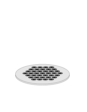
Figure 3: Two dimensional array of planar traps consisting of printed electrodes on a base substrate made of isolating material. Each trap is supposed to be loaded with an electron cloud which is afterwards reduced to a single electron via a sequence of pulses.

II.3 Array of planar traps

The planar structure of the novel trap strongly suggests a 2D array of such traps, as schematically illustrated in Fig. 3. Thin-film technology can be used to place gold electrodes on an isolating surface with resolution much below the mm scale. A large number of traps can be embedded in a common isolating substrate and controlled electronically from the rear side. Ideally each trap is filled with a single electron, which interacts with neighboring particles via the Coulomb force. This provides a natural multiparticle scenario similar to the case of ions in a linear Paul trap, with the advantage of controlling each trap parameter independently (inter-particle distance, coordination number, electron resonance frequencies, …). With the planar trap this is implemented in a very straightforward way.

The substrate shown in Fig. 3 has the size of a coin and each trap a dimension of order 1 mm. This size gives an axial frequency up to 500 MHz for applied voltages of a few Volts. The space between traps has to be filled with a common grounded electrode, so as to isolate the potentials of each trap from the others and also to prevent charging up of the isolating substrate. Thin-layer techniques allows to produce electrodes which are almost monocristalline, and so to reduce significantly the decoherence effect due to patch fields. On the other hand, quantitative measurements of decoherence caused by proximity to the electrodes could be performed by moving the electron along the $z$ axis (see stahl ).

Currently, we are testing a prototype of planar trap. The idea is to have only one trap, with a radius of 2 cm, printed with thick-layer technology over a Al₂O₃ substrate. A magnetic field of 100 G is foreseen. This preliminary trap will try to demonstrate confinement and also the possibility to excite each degree of freedom of the electrons. Figure 4 shows the design of such a test trap. It can be seen that there is a split electrode, which will provide quadrupolar excitation.

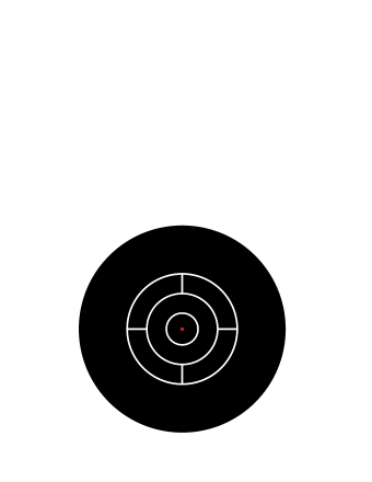
Figure 4: Test trap with total diameter of 35 mm. Black regions denote electrodes and white regions denote isolating surface. As said before the isolating surface has been mostly covered by electrodes to avoid charging up. This configuration has three active electrodes plus an external grounded one. The red circle in the center is a hole through which electrons are loaded from the rear side.

In a further step, we plan to build a miniaturised array of several traps (three for example) in a cryogenic environment of about 100 mK with a magnetic field of 7 Tesla. The traps will have a diameter of around 0.5 mm. The biggest challenges will be those of coherent and accurate control over each electron plus a sufficient supression of all sources of decoherence, both haunting every experiment in quantum computation.

III Building an artificial molecule

III.1 The magnetic gradient

Let us consider a planar trap at a distance $x_{0}$ from the center of the substrate along the $x$-direction. We choose the origin of our reference frame at the substrate center and the $z$-axis orthogonal to the substrate plane (see Fig. 5). Now we suppose to add the inhomogeneous magnetic field

$${\bf{B_{1}}}=b\left(z{\bf{\hat{k}}}-\frac{x}{2}{\bf{\hat{i}}}-\frac{y}{2}{\bf{\hat{j}}}\right).$$ (2)

This field produces a linear magnetic gradient and has rotational symmetry with respect to the $z$-axis.
The total magnetic field acting on the trapped particle is $\bf{B}=\bf{B_{0}}+\bf{B_{1}}$ where $\bf{B_{0}}$ is the uniform confining field directed along the $z$-axis. Hence, the total field $\bf{B}$ acting on the trap center is the sum of the uniform field $B_{0}$ along the $z$-direction and the magnetic gradient $-bx_{0}/2$ along the $x$-direction. Consequently $\bf{B}$, at the trap center, has modulus $B_{c}\equiv\sqrt{B_{0}^{2}+(b^{2}x_{0}^{2})/4}$ and direction forming an angle with the $z$-axis. Note that $B_{c}$ depends on the distance $|x_{0}|$ of the trap from the substrate center.

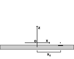
Figure 5: Schematic draw of a planar trap at the distance $x_{0}$ from the center of the substrate.

Now we rotate the reference frame around the $y$-axis so that the new $z$-axis corresponds to the direction of the total magnetic field $\bf{B}$ at the trap center. With this rotation, if $b|x_{0}|/2B_{0}\ll 1$, the total field with respect to the new coordinates can be written, in good approximation, as

$${\bf{B}}\simeq\left[(B_{c}+bz){\bf{\hat{k}}}-\frac{b(x-x_{0})}{2}{\bf{\hat{i}}}-\frac{by}{2}{\bf{\hat{j}}}\right].$$ (3)

The vector potential of the total magnetic field $\bf{B}$ applied to the electron is

$${\bf{A}}\simeq\frac{1}{2}(B_{c}+bz)[(x-x_{0}){\bf{\hat{j}}}-y{\bf{\hat{i}}}].$$ (4)

We suppose to work with a uniform field $B_{0}$ of few Tesla, a magnetic gradient $b$ of about 50 T/m and a trap substrate with length of the order of $10^{-2}$m. Consequently we have $b|x_{0}|/2B_{0}<10^{-1}$.

Let us write the Hamiltonian of the trapped electron. By taking into account the trapping potential we have

$$H=\frac{(\mathbf{p}-e\mathbf{A})^{2}}{2m_{e}}+eV-\frac{ge\hbar}{4m_{e}}\mbox{ \boldmath$\sigma$ }\cdot\mathbf{B},$$ (5)

where $V$, $m_{e}$, $e$, $g$, and $\sigma_{i}$ are, respectively, the trapping potential, electron mass, electron charge, giromagnetic factor, and Pauli matrices. In the limit $b|x_{0}|/2B_{0}\ll 1$ we can neglect the changes in the quadrupole potential form due to the rotation of the reference frame around the $z$-axis and write

$$V\simeq\frac{V_{0}}{\ell^{2}}\left[z^{2}-\frac{(x-x_{0})^{2}+y^{2}}{2}\right].$$ (6)

We can define the axial frequency $\omega_{z}\equiv\sqrt{2eV_{0}/(m_{e}\ell^{2})}$, in terms of the applied potential difference $V_{0}$ and of the characteristic trap size $\ell$, and recast the $z$-part of the spatial Hamiltonian of the electron as

$$H_{z}\simeq\frac{p_{z}^{2}}{2m_{e}}+\frac{1}{2}m_{e}\omega_{z}^{2}z^{2}.$$ (7)

The presence in the Penning trap of the magnetic gradient along the $z$-direction makes the cyclotron frequency depend on the particle $z$-position. Indeed, we define the cyclotron frequency as

$$\omega_{c}(z)\equiv\frac{|e|(B_{c}+bz)}{m_{e}}$$ (8)

and introduce respectively the cyclotron and magnetron ladder operators

$$a_{c} = \frac{1}{2}\left\{\sqrt{\frac{m\tilde{\omega}_{c}}{2\hbar}}\,[(x-x_{0})-iy]+\sqrt{\frac{2}{\hbar m\tilde{\omega}_{c}}}\,(p_{y}+ip_{x})\right\},$$ (9)

$$a_{m} = \frac{1}{2}\left\{\sqrt{\frac{m\tilde{\omega}_{c}}{2\hbar}}\,[(x-x_{0})+iy]-\sqrt{\frac{2}{\hbar m\tilde{\omega}_{c}}}\,(p_{y}-ip_{x})\right\},$$ (10)

obeying the commutation relation $[a_{i},a_{j}^{\dagger}]=\delta_{i,j}$, with $i,j=c,m$. The frequency $\tilde{\omega}_{c}$ is defined as

$$\tilde{\omega}_{c}(z)\equiv\sqrt{\omega_{c}^{2}-2\omega_{z}^{2}},$$ (11)

so it depends on the $z$-coordinate too.

The part of the spatial Hamiltonian of the electron involving $x$-$y$ coordinates is

$$H_{xy} \simeq \frac{1}{2m_{e}}\left[p_{x}+\frac{e(B_{c}+bz)}{2}y\right]^{2}+\frac{1}{2m_{e}}\left[p_{y}-\frac{e(B_{c}+bz)}{2}(x-x_{0})\right]^{2}$$ (12)

$$- \frac{1}{4}m_{e}\omega_{z}^{2}[(x-x_{0})^{2}+y^{2}].$$

By using the ladder operators, Eqs. (9) and (10), we can write

$$H_{xy}=-\hbar\omega_{m}\left(a_{m}^{\dagger}a_{m}+\frac{1}{2}\right)+\hbar\omega^{\prime}_{c}\left(a_{c}^{\dagger}a_{c}+\frac{1}{2}\right),$$ (13)

where we have introduced, respectively, the magnetron and cyclotron frequencies

$$\omega_{m}(z)\equiv\frac{(\omega_{c}-\tilde{\omega}_{c})}{2},$$ (14)

$$\omega^{\prime}_{c}(z)\equiv\frac{(\omega_{c}+\tilde{\omega}_{c})}{2},$$ (15)

both depending, by means of relations (8) and (11), on the $z$-coordinate. Notice that we indicate the explicit dependence of the frequencies $\omega_{c}$, $\tilde{\omega}_{c}$, $\omega^{\prime}_{c}$, and $\omega_{m}$ on the coordinate $z$ only in the definition formula.

The uniform magnetic field of few Tesla, we suppose to apply, gives a cyclotron frequency at the trap center of the order of $100$ GHz. This choice permits to have, after thermalization with a trap environment at about $100$ mK, the cyclotron motion in the lowest energy state gabrielse . Furthermore we choose the axial frequency in the range of MHz, giving a magnetron frequency at the trap center of the order of hundreds of Hz.

The spatial Hamiltonian, Eq. (13), is formally equivalent to the corresponding part of the Hamiltonian describing an electron in a conventional Penning trap, without any magnetic gradient brown . However, we point out that, with respect to the case of a trap without magnetic gradient, there is a dependence of the magnetron and cyclotron frequencies on the $z$-coordinate. Hence, we have a coupling between the axial motion and the cyclotron/magnetron motions. Furthermore, as we shall see, the magnetic gradient introduces an interaction between the spatial motion and the spin motion of the electron. This coupling between the external and internal degrees of freedom becomes evident by considering the part of the electron Hamiltonian involving the spin motion

$$H_{s}\simeq\frac{ge\hbar}{4m_{e}}\mbox{\boldmath$\sigma$ }\cdot\mathbf{B}=\frac{g\hbar}{4}\omega_{c}\sigma_{z}-\frac{g\hbar|e|b}{8m_{e}}(\sigma_{x}x+\sigma_{y}y).$$ (16)

We generally suppose, in our system, the axialization of the electron motion. This condition has been experimentally obtained with ions confined in a Penning trap powell . The motion of the electron is axialized when its amplitude in the $x$-$y$ direction is much smaller than that in the $z$-direction. The axialization permits to neglect, in the above Hamiltonian, the term proportional to $\sigma_{x}x+\sigma_{y}y$. Indeed, with the typical values chosen for $b$ and $B_{0}$, the spin state transition probability due to this term is negligible in the axialization condition. This can be proved by applying time-dependent perturbation theory.

Hence, the global Hamiltonian (5) of the electron can be rewritten as

$$H \simeq -\hbar\omega_{m}\left(a_{m}^{\dagger}a_{m}+\frac{1}{2}\right)+\hbar\omega^{\prime}_{c}\left(a_{c}^{\dagger}a_{c}+\frac{1}{2}\right)+\frac{p_{z}^{2}}{2m_{e}}+\frac{1}{2}m_{e}\omega_{z}^{2}z^{2}+\frac{g\hbar}{4}\omega_{c}\sigma_{z},$$ (17)

where the frequencies $\omega_{m}$, $\omega^{\prime}_{c}$, $\omega_{c}$ and $\tilde{\omega}_{c}$, as defined in Eqs. (8), (11), (14), and (15), depend on the $z$-coordinate.

We suppose that, throughout the electron motion, the conditions $\omega_{z}\ll\omega_{c}$ and $b|z|/2B_{0}\ll 1$ are verified. Hence, by posing $\omega^{\prime}_{c}\simeq\omega_{c}$, $\omega_{m}\simeq\omega_{z}^{2}/2\omega_{c}$ and expanding the cyclotron and magnetron frequencies in terms of the coordinate $z$, we write the above Hamiltonian as

$$H \simeq -\hbar\omega_{m0}a_{m}^{\dagger}a_{m}+\hbar\omega_{c0}a_{c}^{\dagger}a_{c}+\hbar\omega_{z}a_{z}^{\dagger}a_{z}+\frac{\hbar}{2}\omega_{s0}\sigma_{z}$$ (18)

$$+ \hbar\omega_{z}\varepsilon(a_{z}+a_{z}^{\dagger})\left(\frac{\omega_{m0}}{\omega_{c0}}a_{m}^{\dagger}a_{m}+a_{c}^{\dagger}a_{c}+\frac{g}{4}\sigma_{z}\right),$$

where we have introduced the ladder operator

$$a_{z}\equiv\sqrt{\frac{m_{e}\omega_{z}}{2\hbar}}z+i\sqrt{\frac{1}{2\hbar m_{e}\omega_{z}}}p_{z},$$ (19)

the parameter

$$\varepsilon\equiv\frac{|e|b}{m_{e}\omega_{z}}\sqrt{\frac{\hbar}{2m_{e}\omega_{z}}},$$ (20)

and the frequencies $\omega_{c0}\equiv(|e|B_{c})/m_{e}$, $\omega_{m0}\equiv\omega_{z}^{2}/2\omega_{c0}$, $\omega_{s0}\equiv(g\omega_{c0})/2$.

In Hamiltonian (18) we have also redefined the equilibrium position of the electron in the $z$-direction, as a consequence of the shifts due to the zero point energy of the cyclotron and magnetron oscillators.

The parameter $\varepsilon$ gives, substantially, the ratio between the change in the electron spin energy due to the magnetic gradient and the trapping energy in the $z$-direction. Indeed we can write

$$\varepsilon\simeq\frac{\hbar\partial_{z}\omega_{s}\Delta z}{\hbar\omega_{z}},$$ (21)

where

$$\partial_{z}\omega_{s}\equiv\frac{g|e|b}{2m_{e}}$$ (22)

and

$$\Delta z\equiv\sqrt{\frac{\hbar}{2m_{e}\omega_{z}}}$$ (23)

is the amplitude of the electron axial motion in the ground state. Hence $\partial_{z}\omega_{s}\Delta z$ is roughly the spin frequency variation due to the magnetic gradient when the electron axial motion is in the ground state.

Note that the frequencies $\omega_{c0}$, $\omega_{m0}$ and $\omega_{s0}$ depend on the position of the planar trap on the substrate. Indeed they depend on the distance $x_{0}$ of the trap center from the symmetry axis of the magnetic gradient. For instance, when the magnetic gradient $b\simeq 50$ T/m, two electrons in neighboring traps, separated by a distance of the order of $10^{-3}$ m, are characterized by spin resonance frequencies that differ from each other of few MHz. This value, though small in comparison with the typical spin frequency $\omega_{s0}/2\pi\sim 100$ GHz of a single electron, is enough to individually address the spin qubits via microwave radiation. Moreover, the same substrate can accomodate tens of qubits, with frequencies spread over a range of hundred MHz.

If the electron motion is axialized and the cyclotron oscillator remains always in the ground state, we can neglect, in Hamiltonian (18), the term proportional to $(a_{z}+a_{z}^{\dagger})[(\omega_{m0}/\omega_{c0})a_{m}^{\dagger}a_{m}+a_{c}^{\dagger}a_{c}]$. Hence, under these conditions, we can write the Hamiltonian of the system as

$$H \simeq -\hbar\omega_{m0}a_{m}^{\dagger}a_{m}+\hbar\omega_{c0}a_{c}^{\dagger}a_{c}+\hbar\omega_{z}a_{z}^{\dagger}a_{z}+\frac{\hbar}{2}\omega_{s0}\sigma_{z}+\frac{g}{4}\hbar\omega_{z}\varepsilon(a_{z}+a_{z}^{\dagger})\sigma_{z},$$ (24)

showing the coupling between the axial and the spin degrees of freedom.

III.2 Effective spin-spin coupling

We now move to a linear array of $N$ electrons confined in planar Penning traps along the $x$-axis. If we add a linear magnetic gradient, the Hamiltonian of the system can be written as

$$H=\sum_{i=1}^{N}\left[\frac{(\mathbf{p_{i}}-e\mathbf{A_{i}})^{2}}{2m_{e}}+eV_{i}-\frac{ge\hbar}{4m_{e}}{\bf{\sigma_{i}}}\cdot\mathbf{B_{i}}\right]+\sum_{i>j}^{N}\frac{e^{2}}{4\pi\epsilon_{0}|\mathbf{r_{i}}-\mathbf{r_{j}}|},$$ (25)

where the subscript $i$ refers to the $i$-th electron of the array.

Hence the magnetic field $\mathbf{B_{i}}$, with vector potential $\mathbf{A_{i}}$, acts on the electron trapped in the $i$-th site. This field is the sum of the uniform confining field orthogonal to the planar trap substrate and the inhomogeneous field producing a linear magnetic gradient [see derivation of Eq. (3) in the previous subsection]

$${\bf{B_{i}}}\simeq\left[(B_{c,i}+bz_{i}){\bf{\hat{k}}}-\frac{b(x_{i}-x_{i,0})}{2}{\bf{\hat{i}}}-\frac{by_{i}}{2}{\bf{\hat{j}}}\right].$$ (26)

In the above equation $B_{c,i}\bf{\hat{k}}$ is the total field $\mathbf{B_{i}}$ at the center of the $i$-th trap and $x_{i,0}$ is the $x$-coordinate of the center of the $i$-th trap. The origin of our reference frame is at the center of the trap substrate and the $z$-axis is the symmetry axis of the magnetic gradient. We have $B_{c,i}=\sqrt{B_{0}^{2}+(b^{2}x_{i,0}^{2})/4}$ where $|x_{i,0}|$ is the distance between the symmetry axis of the magnetic gradient and the center of the $i$-th site. In writing Eq. (26) we assumed that $b|x_{0,i}|/2B_{0}\ll 1$ for any $i=1,2,\ldots,N$.

Similarly to the single electron case, we also have

$${\bf{A}_{i}}\simeq\frac{1}{2}(B_{c,i}+bz_{i})[(x_{i}-x_{i,0}){\bf{\hat{j}}}-y_{i}{\bf{\hat{i}}}].$$ (27)

and

$$V_{i}\simeq\frac{V_{0}}{\ell^{2}}\left[z_{i}^{2}-\frac{(x_{i}-x_{i,0})^{2}+y_{i}^{2}}{2}\right].$$ (28)

Now, as already done for a single electron in a planar trap in the presence of a magnetic gradient, we define the frequencies $\omega_{c,i}(z_{i})\equiv|e|(B_{c,i}+bz_{i})/m_{e}$ and $\tilde{\omega}_{c,i}(z_{i})\equiv\sqrt{\omega_{c,i}^{2}-2\omega_{z}^{2}}$ and introduce the operators

$$a_{c,j} = \frac{1}{2}\left\{\sqrt{\frac{m_{e}\tilde{\omega}_{c,j}}{2\hbar}}\,[(x_{j}-x_{j,0})-iy_{j}]+\sqrt{\frac{2}{\hbar m_{e}\tilde{\omega}_{c,j}}}\,(p_{y,j}+ip_{x,j})\right\},$$ (29)

$$a_{m,j} = \frac{1}{2}\left\{\sqrt{\frac{m_{e}\tilde{\omega}_{c,j}}{2\hbar}}\,[(x_{j}-x_{j,0})+iy_{j}]-\sqrt{\frac{2}{\hbar m_{e}\tilde{\omega}_{c,j}}}\,(p_{y,j}-ip_{x,j})\right\},$$ (30)

$$a_{z,j} = \sqrt{\frac{m_{e}\omega_{z}}{2\hbar}}z_{j}+i\sqrt{\frac{1}{2\hbar m_{e}\omega_{z}}}p_{z,j}$$ (31)

obeying the commutation relation $[a_{i},a_{j}^{\dagger}]=\delta_{i,j}$, with $i,j=c,m,z$.

If we indicate with $H^{NC}$ the part of Hamiltonian (25) not including the Coulomb interaction, we can write

$$H^{NC} \simeq \sum_{i=1}^{N}\left(-\hbar\omega_{m0,i}a_{m,i}^{\dagger}a_{m,i}+\hbar\omega_{c0,i}a_{c,i}^{\dagger}a_{c,i}+\hbar\omega_{z}a_{z,i}^{\dagger}a_{z,i}+\frac{\hbar}{2}\omega_{s0,i}\sigma_{z,i}\right)$$ (32)

$$+ \sum_{i=1}^{N}\frac{g}{4}\hbar\omega_{z}\varepsilon(a_{z,i}+a_{z,i}^{\dagger})\sigma_{z,i},$$

where we have introduced the frequencies $\omega_{c0,i}\equiv(|e|B_{c,i})/m_{e}$, $\omega_{m0,i}\equiv\omega_{z}^{2}/2\omega_{c0,i}$, $\omega_{s0,i}\equiv(g\omega_{c0,i})/2$ and assumed that, throughout the electron motion, the conditions $\omega_{z}\ll\omega_{c,i}$ and $b|z_{i}|/2B_{0}\ll 1$ are verified for any $i=1,2,\ldots,N$. The parameter $\varepsilon$ has been defined in Eq. (20). In writing Hamiltonian (32) we have also supposed that all the electron motions are axialized and that the cyclotron oscillator remains always in the ground state.

Let us consider the part of Hamiltonian (25) involving the Coulomb interaction between the two electrons at the sites $i$ and $j$. By indicating it with $H^{C}_{i,j}$ we have

$$H^{C}_{i,j}=\frac{e^{2}}{4\pi\epsilon_{0}\sqrt{(x_{i}-x_{j})^{2}+(y_{i}-y_{j})^{2}+(z_{i}-z_{j})^{2}}},$$ (33)

which we can recast as

$$H^{C}_{i,j}=\frac{e^{2}}{4\pi\epsilon_{0}d_{i,j}}\left[1+\frac{2(\Delta x_{i}-\Delta x_{j})}{d_{i,j}}+\frac{(\Delta x_{i}-\Delta x_{j})^{2}}{d_{i,j}^{2}}+\frac{(y_{i}-y_{j})^{2}}{d_{i,j}^{2}}+\frac{(z_{i}-z_{j})^{2}}{d_{i,j}^{2}}\right]^{-\frac{1}{2}},$$ (34)

where $\Delta x_{i}\equiv x_{i}-x_{i,0}$ and $d_{i,j}=|x_{i,0}-x_{j,0}|$.

If the oscillation amplitude of the two electrons is much smaller than the average separation $d_{i,j}$ between them, we can expand the interaction Hamiltonian, Eq. (34), in a power series and retain the terms up to the second order

$$H^{C}_{i,j}\simeq-\frac{e^{2}}{4\pi\epsilon_{0}d_{i,j}^{2}}(\Delta x_{i}-\Delta x_{j})+\frac{e^{2}}{8\pi\epsilon_{0}d_{i,j}^{3}}\left[2(\Delta x_{i}-\Delta x_{j})^{2}-(y_{i}-y_{j})^{2}-(z_{i}-z_{j})^{2}\right].$$ (35)

Furthermore, if we suppose that the electron motions are axialized, we have

$$H^{C}_{i,j}\simeq-\frac{e^{2}}{4\pi\epsilon_{0}d_{i,j}^{2}}(\Delta x_{i}-\Delta x_{j})-\frac{e^{2}}{8\pi\epsilon_{0}d_{i,j}^{3}}(z_{i}-z_{j})^{2}.$$ (36)

The first term in Hamiltonian (36) gives a displacement of the equilibrium position of the electrons along the $x$-axis. This small shift is of order of $e^{2}/(4\pi\epsilon_{0}d_{i,j}^{2}m_{e}\omega_{c0,i}^{2})$ and is a consequence of the Coulomb repulsion. Hence we can effectively remove the first term in Hamiltonian (36) by redefining the centers of the two traps. We also recall that, actually, this effect is more pronounced for electrons placed at the extremities of the array. Indeed, as a consequence of the symmetry of the system, particles trapped near the center of the array undergo much smaller shifts.

The second term in Hamiltonian (36), involving the $z$-coordinate of the electrons, represents an effective dipole-dipole interaction between the $i$-th and $j$-th electrons. By developing the square we have terms proportional to $z_{i}^{2}$ and $z_{j}^{2}$. They produce small shifts on the axial frequencies of the two electrons. Therefore we can take into account these terms by appropriately redefining the axial frequencies of the two electrons. The remaining term, proportional to $z_{i}z_{j}$ represents the Coulomb coupling between the axial motion of the two electrons. After having appropriately redefined the trap centers and frequencies we can write

$$H^{C}_{i,j}\simeq\frac{e^{2}}{4\pi\epsilon_{0}d_{i,j}^{3}}z_{i}z_{j}=\hbar\xi_{i,j}(a_{z,i}+a^{\dagger}_{z,i})(a_{z,j}+a^{\dagger}_{z,j}),$$ (37)

where

$$\hbar\xi_{i,j}\equiv\frac{e^{2}}{4\pi\epsilon_{0}d_{i,j}}\left(\frac{\Delta z}{d_{i,j}}\right)^{2},$$ (38)

with $\Delta z$ being the ground state amplitude of the axial oscillator, introduced in Eq. (23).

Now we perform, on the global Hamiltonian of the system $H=H^{NC}+\sum_{i>j}^{N}H^{C}_{i,j}$, the unitary transformation $H^{\prime}=e^{S}He^{-S}$ mintert with

$$S=\sum_{i=1}^{N}\varepsilon\frac{g}{4}(a_{z,i}^{\dagger}-a_{z,i})\sigma_{z,i}.$$ (39)

The transformed axial operators are

$$a_{z,i}\rightarrow a_{z,i}-\varepsilon\frac{g}{4}\sigma_{z,i}.$$ (40)

Let us consider the transformed part of the Hamiltonian (25) not including the Coulomb terms. It can be written, after dropping constant terms, as

$$H^{\prime NC} \simeq \sum_{i=1}^{N}\left(-\hbar\omega_{m0,i}a_{m,i}^{\dagger}a_{m,i}+\hbar\omega_{c0,i}a_{c,i}^{\dagger}a_{c,i}+\hbar\omega_{z}a_{z,i}^{\dagger}a_{z,i}+\frac{\hbar}{2}\omega_{s0,i}\sigma_{z,i}\right)$$ (41)

Note that, with the unitary transformation, we have formally removed the interaction between the axial and spin motions. Differently the Coulomb terms in Hamiltonian (25) involving the electrons $i$ and $j$ transform as

$$H^{\prime C}_{i,j} = \hbar\xi_{i,j}\left(a_{z,i}+a^{\dagger}_{z,i}-\varepsilon\frac{g}{2}\sigma_{z,i}\right)\left(a_{z,j}+a^{\dagger}_{z,j}-\varepsilon\frac{g}{2}\sigma_{z,j}\right).$$ (42)

From the above Hamiltonian we see that the unitary transformation produces terms of the form $\hbar(g^{2}/4)\varepsilon^{2}\xi_{i,j}\sigma_{z,i}\sigma_{z,j}$, which represent an effective coupling between the spin motion of different particles.

By applying another unitary transformation, similar to Eq. (39), also the extra terms in Hamiltonian (42), proportional to $\sigma_{z,i}(a_{z,j}+a^{\dagger}_{z,j})$, result in additional spin-spin coupling terms. As a consequence we would have corrections to the coupling strength of the spin-spin interaction the order of $\hbar\varepsilon^{2}\xi_{i,j}^{3}/\omega_{z}^{2}$. However, we assume $\xi_{i,j}\ll\omega_{z}$, so that the effect due to the terms proportional to $\sigma_{z,i}(a_{z,j}+a^{\dagger}_{z,j})$ is negligible.

Since in our scheme quantum information is encoded only in the spin motion of the particles, we do not consider the spatial part of the transformed Hamiltonian, but just the spin-part, given by

$$H^{\prime}_{s} \simeq \sum_{i=1}^{N}\frac{\hbar}{2}\omega_{s0,i}\sigma_{z,i}+\sum_{i>j}^{N}\frac{\hbar}{2}\pi J_{i,j}\sigma_{z,i}\sigma_{z,j}.$$ (43)

Note that the above Hamiltonian is analogous to the nuclear spin Hamiltonian of the molecules used to perform NMR quantum computation jones . Consequently, with our system, we can implement universal quantum processing by using the same techniques developed in NMR experiments (see next section).

In Hamiltonian (43) the spin frequencies are

$$\omega_{s0,i}\simeq\frac{geB_{0}}{2m_{e}}\left(1+\frac{b^{2}x_{i,o}^{2}}{8B_{0}^{2}}\right)$$ (44)

and the coupling constants, defined as in NMR experiments, are

$$J_{i,j}\equiv\frac{g^{2}}{2\pi}\xi_{i,j}\varepsilon^{2}=\frac{g^{2}}{2\pi\hbar}\frac{e^{2}}{4\pi\epsilon_{0}d_{i,j}}\left(\frac{\Delta z}{d_{i,j}}\right)^{2}\left(\frac{\hbar\partial_{z}\omega_{s}\Delta z}{\hbar\omega_{z}}\right)^{2}\propto\frac{b^{2}}{\omega_{z}^{4}d_{i,j}^{3}}.$$ (45)

Hence, by changing specific system parameters, fully under the control of the experimenter, we can adjust both the spin frequencies and the coupling constants. Indeed, according to the above relations, the spin frequencies of the particles and, consequently, their detunings depend on the uniform magnetic field intensity, the magnetic gradient strength and the distance of the electrons from the substrate center. Similarly, the coupling constants can be modified by changing the gradient strength, the axial frequency and the distance between the particles. We also note that the coupling constants are proportional to $1/d_{i,j}^{3}$. Hence, if the particles are equally spaced in the array, we obtain a uniform coupling strength for nearest-neighbor electrons, while the spin-spin interaction decreases rapidly with the increase of their distances. For instance, the coupling strength between two electrons, that are a distance $2d$ apart from each other, is just 1/8 of the one for nearest-neighbor electrons. In the considered dipole limit, we achieve the same uniform interaction strength between neighboring electrons and reduction for non-nearest-neighbor $J$ couplings of Ref. mchugh , where, however, this result requires a careful adjustment of both the inter-ion separation and end-trap strength.

IV Universal quantum logic gates

In this section we describe how to implement, in our system, universal quantum computation.

As mentioned in the previous section, Hamiltonian (43) is substantially analogous to the one describing NMR molecules jones . The only difference is the fact that in the NMR systems we have nuclear spins instead of electron spins. Therefore, universal quantum processing with trapped electrons, in the presence of a magnetic gradient, can be performed by using techniques similar to those already developed in NMR experiments jones .

In particular, Hamiltonian (43) represents a set of $N$ electron spins, each one having a different precession frequency, which interact by mutual couplings. If we encode a qubit in the spin degree of freedom of each particle, we can use electromagnetic pulses with appropriate frequencies to selectively manipulate the information stored in the spin state of each electron. Hence, the detuning between the different electron frequencies plays the same role of the chemical shift in NMR molecules.

Universal two-qubit gates, in our system, are achieved by means of the mutual coupling between the electron spins. Indeed, this interaction has the same form of the $J$-coupling between nuclear spins in NMR molecules and can be used in a similar way to perform two-qubit gates.

The set of unitary transformations consisting of single-qubit gates plus C-NOT gates is computationally universal. Let us describe, in detail, how to perform, in our system, these operations. If we apply a small transverse oscillating magnetic field resonant with the spin precession frequency $\omega_{s0,j}$ of the $j$-th electron

$${\bf B_{d}}(t)=B_{d}[{\bf{\hat{i}}}\cos(\omega_{s0,j}t+\theta)+{\bf{\hat{j}}}\sin(\omega_{s0,j}t+\theta)],$$ (46)

the relevant part of the system Hamiltonian becomes, in interaction picture with respect to the unperturbed Hamiltonian $H_{s0}=\sum_{i=1}^{N}(\hbar/2)\omega_{s0,i}\sigma_{z,i}$ and in rotating wave approximation,

$$H_{IP}^{(spin)}\simeq\hbar\frac{\chi}{2}\left(\sigma_{+,j}e^{-i\theta}+\sigma_{-,j}e^{i\theta}\right),$$ (47)

where $\chi\equiv g|e|B_{d}/(2m_{e})$ and $\sigma_{\pm,j}\equiv(\sigma_{x,j}\pm i\sigma_{y,j})/2$.
In the derivation of the above Hamiltonian we neglected the spin-spin coupling terms present in Hamiltonian (43), since we assume $J_{i,j}\ll\chi$ for any $i,j=1,2,\ldots,N$. Furthermore we suppose that the oscillating field is so small that $B_{d}\ll bd_{i,j}$ for any $i,j=1,2,\ldots,N$. This last condition, giving a Rabi frequency $\chi$ much smaller than the detuning between the spin frequencies of the $i$-th and $j$-th electrons, allows for the selective frequency addressing of each particle.

If the small transverse magnetic field is applied for a time $t$, it produces a rotation on the spin state of the $j$-th particle

$$|\downarrow\rangle_{j} \rightarrow \cos\left(\frac{\chi t}{2}\right)|\downarrow\rangle_{j}-ie^{-i\theta}\sin\left(\frac{\chi t}{2}\right)|\uparrow\rangle_{j},$$ (48)

$$|\uparrow\rangle_{j} \rightarrow \cos\left(\frac{\chi t}{2}\right)|\uparrow\rangle_{j}-ie^{i\theta}\sin\left(\frac{\chi t}{2}\right)|\downarrow\rangle_{j}.$$ (49)

It can be shown that with an appropriate combination of these operations, one can perform any single-qubit gate on the spin qubit of the $j$-th electron. We define the interaction produced by the Hamiltonian (47), applied for a time $t$, as a $p_{s,j}(\chi t,\theta)$ pulse. Hence, we can perform single-qubit gates on each electron, in a selective way, by appropriately tuning the frequency of the oscillating magnetic field.

Let us now consider the implementation of C-NOT gates. A natural way to perform this two-qubit gate is to use a three gate circuit. In particular, we apply in sequence, an Hadamard gate on the target qubit, a controlled $\pi$ phase-shift gate followed by another Hadamard gate on the target qubit. However, it is preferable to avoid Hadamard gates, as they are difficult to implement. Hence, the Hadamard gates are conveniently replaced by an inverse pseudo-Hadamard gate and a pseudo-Hadamard gate jones . These two gates are realized by applying respectively a $p_{s}(\pi/2,\pi/2)$ pulse and a $p_{s}(\pi/2,-\pi/2)$ pulse. The controlled $\pi$ phase-shift gate can be achieved, in different ways, by applying appropriate sequences of $p_{s}$ pulses. For example, in a two-qubit system, one possible sequence for implementing this gate consists of four $p_{s}$ pulses and two appropriately timed periods of free evolution jones . In particular, we apply: a free evolution of the system for a time of $1/4J_{1,2}$, a $p_{s}(\pi,0)$ pulse, another free evolution of the system for a time of $1/4J_{1,2}$, a $p_{s}(\pi/2,0)$ pulse, a $p_{s}(\pi/2,\pi/2)$ pulse and a $p_{s}(\pi/2,0)$ pulse. All the above pulses should be applied to both electron spins and the application time of each $p_{s}$ pulse should be much smaller than the time duration of each free evolution period.

With systems having more than two qubits, the efficient implementation of C-NOT gates requires the application of more complicated sequences of operations. This is necessary in order to avoid errors due to the couplings with electrons not involved in the gates. Indeed, from Hamiltonian(43) we see that there are mutual couplings among all the particles of the system. However, the sequence required to efficiently implement the C-NOT gates, when we have more than two qubits, consists only of $p_{s}$ pulses acting on specific particles and appropriately timed periods of free evolution jones2 ; leung . In NMR context this technique is known as refocusing.

We also remark that in our system the coupling strength decreases rapidly with the increase of the inter-particle distance. Indeed from equation (45) we have $J_{i,j}\propto 1/d_{i,j}^{3}$. This fact permits to simplify the refocusing sequences since the interaction between distant electrons can be neglected jones2 ; linden . We recall that in this case the logic gates between distant electrons can be performed by means of swap gates, which move the quantum information among the particles. A swap gate is realized by applying three C-NOT gates, where the two qubits play alternatively the role of target and controller.

Let us give realistic estimates for the values of the electron detunings and spin-spin couplings achievable in our system. We consider a linear array of $10$ electrons with inter-particle distance of the order of $1$mm. We suppose to apply a uniform magnetic field of few Tesla, giving $\omega_{s}/2\pi\approx 100$ GHz, a magnetic gradient of about 50 T/m and assume an axial frequency $\omega_{z}/2\pi\approx 10$ MHz. In these conditions we obtain a frequency detuning between neighboring particles of few MHz and a spin-spin coupling with strength $J\approx 20$ Hz. These values for the detuning and the coupling strength are of the same order of the corresponding quantities in NMR systems.

V Conclusion

A novel concept of open planar Penning trap makes it possible to design and build-up a scalable system for quantum computation, consisting of trapped electrons in vacuum. Single particles are confined in a linear array of traps, deposited on the same substrate. A magnetic field gradient across the traps allows for frequency addressing of each qubit, stored into the electron spin as in NMR quantum computers. Moreover, the magnetic field gradient couples internal (spin) and external (motional) degrees of freedom of the same particle. Thanks to the Coulomb interaction among the charged particles, this coupling effectively amounts to a direct spin-spin interaction, with tunable coupling strength. In the limit of relatively large inter-electron spacing and small axial oscillation amplitude, we obtain an analytical expression for the $J$ coupling, which allows for an immediate evaluation of the interaction strength in terms of the relevant system parameters (trap distance, axial frequency, and applied magnetic gradient). We emphasize that the $J$ coupling is proportional to $1/d^{3}$, where $d$ is the inter-trap distance, thus greatly reducing the interaction between non-nearest-neighbor electrons.

This way, the system of singly trapped electrons is formally identical to a NMR molecule, suitable for quantum information processing. Hence, the well established and developed techniques of NMR spectroscopy can be extended and applied to our system. Qubit manipulation is achieved via appropriate sequences of microwave pulses. The qubit read-out is performed either by axial frequency detection, as in conventional Pennning traps, or by capacity and charge measurements as in semiconductor quantum dots.

The advantages over NMR systems are obvious: the number of qubits is not limited neither by the molecule size – the same substrate can easily accomodate a large number of microtraps – nor by the frequency range – the typical spin resonance frequency lies in the GHz, whereas the detuning between neighboring particles is of the order of a few kHz –, and the system is truly quantum and, at the same time, well isolated from the environment. In addition, the geometry of the system can be designed and optmized at will, using more complicated two dimensional arrays, with possible applications to the study and the simulation of quantum systems like the Ising model. Finally, Penning traps could be loaded with protons as well, allowing the same NMR spectroscopy experiments with hydrogen, but in a much more controlled and clean environment.

- (1) J.A. Jones, Prog. NMR Spectroscop. 38, 325 (2001).
- (2) D. Leibfried, R. Blatt, C. Monroe, and D. Wineland, Rev. Mod. Phys. 75, 281 (2003).
- (3) S. Gulde, M. Riebe, G.P.T. Lancaster, C. Becher, J. Eschner, H. Häffner, F. Schmidt-Kaler, I.L. Chuang, and R. Blatt, Nature 421, 48 (2003).
- (4) D. Leibfried, B. DeMarco, V. Meyer, D. Lucas, M. Barrett, J. Britton, W.M. Itano, B. Jelenkovic, C. Langer, T. Rosenband, and D.J. Wineland, Nature 422, 412 (2003).
- (5) F. Mintert and Ch. Wunderlich, Phys. Rev. Lett. 87, 257904 (2001).
- (6) Ch. Wunderlich, in Laser Physics at the Limit, p. 261 (Springer, Heidelberg, 2001).
- (7) Ch. Wunderlich and Ch. Balzer, in Advances in Atomic, Molecular and Optical Physics, (Academic Press, San Diego, Ca, 2003).
- (8) Ch. Wunderlich, Ch. Balzer, T. Hannemann, F. Mintert, W. Neuhauser, D. Reiß, and P.E. Toschek, J. Phys. B: At. Mol. Opt. Phys. 36, 1063 (2003).
- (9) D. Mc Hugh and J. Twamley, Phys. Rev. A 71, 012315 (2005).
- (10) G. Ciaramicoli, I. Marzoli, and P. Tombesi, Phys. Rev. Lett. 91, 017901 (2003).
- (11) G. Ciaramicoli, I. Marzoli, and P. Tombesi, Phys. Rev. A 70, 032301 (2004).
- (12) S. Stahl, F. Galve, J. Alonso, S. Djekic, W. Quint, T. Valenzuela, J. Verdù, M. Vogel, and G. Werth, Eur. Phys. J. D 32, 139 (2005).
- (13) F. G. Major, V. Gheorghe, G. Werth, Charged Particle Traps, (Springer, Heidelberg, 2005).
- (14) E. A. Cornell, R. M. Weisskoff, K. R. Boyce and D. E. Pritchard, Phys. Rev. A 41, 312 (1990).
- (15) J. Verdú et al., Physica Scripta T112, 68 (2004).
- (16) S. Djekic et al., accepted for Eur. Phys. J. D.
- (17) J.R. Anglin and W.H. Zurek, arXiv:quant-ph/9611049; C. Henkel, S. Pötting, and M. Wilkens, Appl. Phys. B 69, 379 (1999).
- (18) M. Diederich et al., Hyperfine Interactions 115, 185 (1998).
- (19) J.D. Jackson, Classical Electrodynamics, 2nd ed., (Wiley, New York, 1975).
- (20) S. Peil and G. Gabrielse, Phys. Rev. Lett. 83, 1287 (1999).
- (21) L.S. Brown and G. Gabrielse, Rev. Mod. Phys. 58, 233 (1986).
- (22) H.F. Powell, D.M. Segal, and R.C. Thompson, Phys. Rev. Lett. 89, 093003 (2002).
- (23) J.A. Jones and E. Knill, J. Magn. Reson. 141, 322 (1999).
- (24) D.W. Leung, I.L. Chuang, F. Yamaguchi and Y. Yamamoto, Phys. Rev. A 61, 042310 (2000).
- (25) N. Linden, Ē. Kupc̆e and R. Freeman, Chem. Phys. Lett. 311, 321 (1999).