Non-adiabatic quantum molecular dynamics: Ionization of many electron systems

Abstract

We propose a novel method to describe realistically ionization processes with absorbing boundary conditions in basis expansion within the formalism of the so-called Non-Adiabatic Quantum Molecular Dynamics. This theory couples self-consistently a classical description of the nuclei with a quantum mechanical treatment of the electrons in atomic many-body systems. In this paper we extend the formalism by introducing absorbing boundary conditions via an imaginary potential. It is shown how this potential can be constructed in time-dependent density functional theory in basis expansion. The approach is first tested on the hydrogen atom and the pre-aligned hydrogen molecular ion H${}_{2}^{+}$ in intense laser fields where reference calculations are available. It is then applied to study the ionization of non-aligned H${}_{2}^{+}$ and H₂. Striking differences in the orientation dependence between both molecules are found. Surprisingly, enhanced ionization is predicted for perpendicularly aligned molecules.

I Introduction

The experimental and theoretical investigation of the interaction of atoms, molecules and clusters with intense laser fields represents one of the most challenging problems of current research. In atoms, high harmonic generation (HHG)McPherson et al. (1987); Ferray et al. (1988); Li et al. (1989), above threshold ionization Agostini et al. (1979); Kruit et al. (1983); Fedorov (1997) or stabilization against ionization Pont and Gavrila (1990); de Boer et al. (1993, 1994); Fedorov (1997) have been observed. In molecules, due to the additional nuclear degrees of freedom (DOF), further mechanisms occur, like molecular stabilization against dissociation Yuan and George (1978); Bandrauk and Sink (1981); Posthumus et al. (2000), bond softening Yao and Chu (1993); Charron et al. (1993); Giusti-Suzor et al. (1995); Sändig et al. (2000); Williams et al. (2000), above threshold dissociation Giusti-Suzor et al. (1990); Bucksbaum et al. (1990); Williams et al. (2000), charge resonance enhanced ionization Codling and Frasinski (1993); Zuo and Bandrauk (1995); Seideman et al. (1995); Williams et al. (2000), orientation dependent HHG Yu and Bandrauk (1995); Kopold et al. (1998); Lappas and Marangos (2000); Lein et al. (2002a, b, 2003, b); Kamta and Bandrauk (2004); Zimmermann et al. (2005); Chirilă and Lein (2005), molecular species dependent orientation dependence of single ionization in dimers Litvinyuk et al. (2003); Alnaser et al. (2004); Zhao et al. (2003) or an unexpected suppression of ionization in dimers in comparison to the so-called companion atom Talebpour et al. (1998); Wells et al. (2002); Talebpour et al. (1996); Guo et al. (1998); DeWitt et al. (2001); Faisal et al. (1999); Muth-Böhm et al. (2000); Kjeldsen and Madsen (2004); Dundas and Rost (2005), to name but a few effects.

The theoretical understanding of these mechanisms requires, in principle, the solution of the time-dependent Schrödinger equation (TDSE) for all electrons and all nuclear DOF. However, only for the smallest systems, atomic hydrogen Geltman (2000); Hansen et al. (2001), atomic helium Dundas et al. (1999); Parker et al. (2000), laser aligned H${}_{2}^{+}$ Chelkowski et al. (1995) and laser aligned H₂ with fixed nuclei Harumiya et al. (2000, 2002) numerical solutions of the TDSE exist. In larger systems (or for hydrogen molecules without constraints) approximations are necessary due to the exponential scaling of the computational effort with the number of DOF.

One possibilty consists in the combination of time-dependent density functional theory Runge and Gross (1984) (TDDFT) and a classical description of the nuclei Saalmann and Schmidt (1996); Kunert and Schmidt (2003); Uhlmann et al. (2003); Calvayrac et al. (1998); Suraud and Reinhard (2000); Calvayrac et al. (2000); Dundas (2004); Castro et al. (2004). Most of the approaches use a representation of the Kohn-Sham (KS) functions on a grid to solve the time-dependent KS equations Calvayrac et al. (1998); Suraud and Reinhard (2000); Calvayrac et al. (2000); Castro et al. (2004); Dundas (2004). The first of these grid based approaches has been developed by Reinhard et al. Calvayrac et al. (1998); Suraud and Reinhard (2000); Calvayrac et al. (2000). More recently, Dundas Dundas (2004) and Castro et al. Castro et al. (2004) have also developed such methods.

In contrast, a basis expansion of the KS-orbitals with local basis functions is used in the so-called non-adiabatic quantum molecular dynamics (NA-QMD), developed in our group Saalmann and Schmidt (1996); Kunert and Schmidt (2003). It has been successfully applied so far to very different non-adiabatic processes, like atom-cluster collisions Saalmann and Schmidt (1998), ion-fullerene collisions Kunert and Schmidt (2001), laser induced excitation and fragmentation of molecules Uhlmann et al. (2003) or fragmentation and isomerization of organic molecules in laser fields Kunert et al. (2005). However, a realistic description of ionization with the NA-QMD theory is still an open problem.

In this work, we present a general method in basis expansion and extend the NA-QMD formalism to describe ionization in many-electron systems. To this end, two problems have to be addressed. First, an appropriate basis set suitable for the description of highly excited and ionized states has to be found. We have focused on this problem in a recent paper Uhlmann et al. (2005a). The second problem concerns the introduction of absorbing boundary conditions. This is still a challenging problem for many-electron calculations performed on grids (see e.g. Dundas and Rost (2005)), and in particular, completely open for methods using basis expansion.

In Uhlmann et al. (2003) we have used an ad-hoc manipulation of the electronic expansion coefficients in one electron calculations. In this paper, we introduce general absorbing boundary conditions in basis expansion via an imaginary potential. It will be shown, how such an potential can be build using the many-body Schrödinger equation as well as TDDFT.

The outline of this paper is as follows. First, we introduce absorbing boundary conditions in basis expansion for the general case of the Schrödinger equation in section II.1. In section II.2, the extension of the NA-QMD formalism including absorbing boundary conditions is presented. Details of the used absorbing potential are outlined in section II.3. The method is tested on the hydrogen atom (section III.1) as well as aligned H${}_{2}^{+}$ (section III.2) where reference calculations are available. In section III.3, the calculated ionization probabilities and rates of non-aligned H${}_{2}^{+}$ and H₂ are presented. A completely different orientation dependence between both molecules is found. In addition, the calculations predict surprisingly enhanced ionization for perpendicularly aligned molecules.

II Absorbing boundary conditions

II.1 The Schrödinger equation and basic idea

We start with the introduction of absorbing boundary conditions for the general case of the Schrödinger equation (atomic units are used throughout the paper)

$$\text{i}\frac{\partial}{\partial t}|\Psi\rangle=\hat{H}(t)|\Psi\rangle$$ (1)

where the Hamiltonian

$$\hat{H}(t)=\hat{T}+\hat{V}(t)$$ (2)

consists of the operator for the kinetic energy $\hat{T}$ and the potential $\hat{V}$ which includes the two-body interaction. Thus, $|\Psi\rangle$ represents the, in general, many-particle wave function. The absorbing boundary conditions are incorporated via an imaginary potential. The Hamiltonian is thus modified,

$$\hat{H}_{\text{abs}}(t)=\hat{H}(t)-\text{i}\hat{V}_{\text{abs}}(t)$$ (3)

where $\hat{V}_{\text{abs}}$ is the absorbing potential. With a hermitian $\hat{V}_{\text{abs}}$ such an operator $\hat{H}_{\text{abs}}$ is not hermitian and therefore the norm is not conserved, i.e.

$$\frac{\text{d}}{\text{d}t}\langle\Psi|\Psi\rangle = \langle\Psi|\text{i}\hat{H}_{\text{abs}}^{*}-\text{i}\hat{H}_{\text{abs}}|\Psi\rangle$$ (4)

$$= -2\langle\Psi|\hat{V}_{\text{abs}}|\Psi\rangle\,\text{.}$$

A semi-positive definite $\hat{V}_{\text{abs}}$ leads to the desired effect of norm reduction, i.e. the derivative in (4) is negative or zero.

The balance of the total energy

$$E(t)=\langle\Psi(t)|\hat{H}(t)|\Psi(t)\rangle$$ (5)

is changed if the absorber potential is used in the propagation of $|\Psi\rangle$, i.e.

$$\frac{\text{d}}{\text{d}t}E=\langle\Psi|\frac{\text{d}}{\text{d}t}\hat{V}|\Psi\rangle+\Delta_{\text{abs}}$$ (6)

with

$$\Delta_{\text{abs}}=-\langle\Psi|\hat{V}_{\text{abs}}\hat{H}+\hat{H}\hat{V}_{\text{abs}}|\Psi\rangle\,.$$ (7)

The additional term is due to the absorber potential and changes the energy balance. Its actual effect depends on the definition of the potential $\hat{V}_{\text{abs}}$.

Introducing the time-dependent eigenfunctions $|\chi_{a}\rangle$ to $\hat{H}$

$$\hat{H}(t)|\chi_{a}(t)\rangle=E_{a}(t)|\chi_{a}(t)\rangle$$ (8)

we define the absorbing potential as

$$\hat{V}_{\text{abs}}=\sum_{a=1}^{\infty}f_{a}|\chi_{a}\rangle\langle\chi_{a}|\,\text{.}$$ (9)

The states $|\chi_{a}\rangle$, sometimes called “field-following” adiabatic states Kono et al. (2003, 2004), form an orthonormal set. With our definition of $\hat{V}_{\text{abs}}$ these states $|\chi_{a}\rangle$ are also eigenstates to $\hat{H}_{\text{abs}}$

$$\hat{H}_{\text{abs}}(t)|\chi_{a}(t)\rangle=(E_{a}(t)-\text{i}f_{a})|\chi_{a}(t)\rangle$$ (10)

but lead to imaginary eigenenergies, i.e. finite lifetimes. The factors $f_{a}$ determine the strength of the absorber at a certain energy and are discussed in section II.3. The wave function $|\Psi(t)\rangle$ is now expanded also in these eigenfunctions

$$|\Psi\rangle=\sum_{a=1}^{\infty}a_{a}|\chi_{a}\rangle\,.$$ (11)

Inserted into the time-derivative of the norm (4) this yields

$$\frac{\text{d}}{\text{d}t}\langle\Psi|\Psi\rangle=-2\sum_{a=1}^{\infty}\left|a_{a}\right|^{2}f_{a}$$ (12)

and the additional term $\Delta_{\text{abs}}$ (7) of the energy balance becomes

$$\Delta_{\text{abs}}=-2\sum_{a=1}^{\infty}\left|a_{a}\right|^{2}f_{a}E_{a}\,\text{.}$$ (13)

From equation (12), one can see that the absorber potential decreases the norm of arbitrary wave functions $|\Psi\rangle$ only, if all $f_{a}\geq 0$. Furthermore, it has to be guaranteed that electronic density in bound states is not affected by the absorbing potential. In calculations on spatial grids this is approximately satisfied by applying the absorbing boundary conditions far away from the nuclei (see e.g. Neuhasuer and Baer (1989); Chelkowski et al. (1995); Dundas et al. (2000)). In our case of basis expansion (11), this condition can naturally be fulfilled if the time-dependent eigenvalues $f_{a}$ of $\hat{V}_{\text{abs}}$ (9) are chosen to be

$$f_{a}=\left\{\begin{array}[]{ccc}f_{a}=0&\hskip 14.22636pt\text{if}&E_{a}\leq 0\\ f_{a}>0&\text{if}&E_{a}>0\end{array}\right.\,,$$ (14)

i.e. the absorbing potential acts only on states in the continuum. Thus, $\Delta_{\text{abs}}$ is always zero or negative if the potential is defined as in (9) and if the $f_{a}$ meet the criterion (14).

II.2 Non-Adiabatic Quantum Molecular Dynamics

So far we have shown how to introduce absorbing boundary conditions if the Schrödinger equation in basis expansion is used. We show in the following how to introduce an absorbing potential within the NA-QMD formalism.

The coupled equations of motion (EOM) for the nuclear and electronic system have been given elsewhere in TDDFT Kunert and Schmidt (2003) and time-dependent Hartree-Fock (TDHF) Kunert et al. (2005) and will not be repeated here. Instead we will present the changes in the single-particle EOM arising from an additional imaginary potential in the effective single-particle potential.

The single-particle wave functions are expanded in a local basis

$$\Psi^{j\sigma}(\vec{r},t)=\sum_{\alpha=1}^{N_{\text{b}}}a^{j\sigma}_{\alpha}(t)\phi_{\alpha}(\vec{r}-\vec{R}_{A_{\alpha}}(t))\hskip 28.45274pt\text{with}\hskip 14.22636ptj=1\dots N_{\text{e}}^{\sigma},\,\sigma=\uparrow,\downarrow$$ (15)

and only the expansion coefficients $a^{j\sigma}_{\alpha}(t)$ are explicitly time-dependent. The symbol $A_{\alpha}$ denotes the atom to which the atomic basis function $\phi_{\alpha}$ is attached. The $N_{\text{b}}$ basis functions are either located at the nuclei, which in general move, or are located at fixed positions in space Uhlmann et al. (2005a). $N_{\text{e}}^{\sigma}$ is the number of electrons with the spin $\sigma$.

The variation of the total action with respect to electronic expansion coefficients and nuclear coordinates leads to self-consistently coupled EOM Kunert and Schmidt (2003); Kunert et al. (2005) for the electronic expansion coefficients $a^{j\sigma}_{\alpha}(t)$ and for the nuclear coordinates $\vec{R}_{A}$. Here we add an imaginary potential to the effective single-particle Hamiltonian. The EOM for the electronic expansion coefficients are then modified (cf. with Kunert and Schmidt (2003); Kunert et al. (2005))

$$\frac{\text{d}}{\text{d}t}a^{j\sigma}_{\alpha}=-\sum_{\beta\gamma}^{N_{\text{b}}}\left(S^{-1}\right)_{\alpha\beta}\left(\text{i}H_{\beta\gamma}^{\sigma}+V_{\text{abs,}\beta\gamma}^{\sigma}+B_{\beta\gamma}\right)a^{j\sigma}_{\gamma}\qquad j=1,\dots,N_{\text{e}}^{\sigma},\,\sigma=\uparrow,\downarrow\,\text{.}$$ (16)

In (16)

$$S_{\alpha\beta}=\left\langle\phi_{\alpha}\left|\phi_{\beta}\right.\right\rangle$$ (17)

is the overlap matrix between basis states,

$$H_{{\alpha\beta}}^{\sigma}=\left\langle\phi_{\alpha}\left|\hat{H}_{\text{eff}}^{\sigma}\right|\phi_{\beta}\right\rangle$$ (18)

is the effective Hamilton matrix with $\hat{H}_{\text{eff}}^{\sigma}$ the effective one-particle Hamiltonian Kunert and Schmidt (2003); Kunert et al. (2005),

$$B_{{\alpha\beta}}=\left\langle\phi_{\alpha}\left|\frac{\text{d}}{\text{d}t}\phi_{\beta}\right.\right\rangle$$ (19)

is the non-adiabatic coupling matrix and

$$V_{\text{abs,}{\alpha\beta}}^{\sigma}=\left\langle\phi_{\alpha}\left|\hat{V}_{\text{abs}}^{\sigma}\right|\phi_{\beta}\right\rangle$$ (20)

is the matrix element of the additional absorber potential introduced here and still to be defined (see below).

At this point we note explicitely that the EOM (16) are exactly the same for TDDFT Kunert and Schmidt (2003) and TDHF Kunert et al. (2005). The difference between both approaches consists in the calculation of the matrix elements $H_{\alpha\beta}^{\sigma}$ which in case of TDHF contains the non-local exchange term. Thus, the whole following discussions and derivations belong simultaneously to both approaches, TDDFT Kunert and Schmidt (2003) and TDHF Kunert et al. (2005).

With the additional damping term (20) the time-dependence of the norm (i.e. the total number of electrons in this case) becomes

$$\frac{\text{d}}{\text{d}t}N=\frac{\text{d}}{\text{d}t}\sum_{\sigma=\uparrow,\,\downarrow}\sum_{j=1}^{N_{\text{e}}^{\sigma}}\sum_{{\alpha\beta}=1}^{N_{\text{b}}}a_{\alpha}^{j\sigma*}a_{\beta}^{j\sigma}S_{\alpha\beta}=-2\,\sum_{j\sigma{\alpha\beta}}V_{\text{abs,}{\alpha\beta}}^{\sigma}a_{\alpha}^{j\sigma*}a_{\beta}^{j\sigma}\,.$$ (21)

The total energy reads Kunert and Schmidt (2003)

$$E(t) = U(\vec{R},t)+\sum_{A=1}^{N_{\text{i}}}\frac{M_{A}}{2}\dot{\vec{R}}_{A}^{2}+\sum_{\sigma=\uparrow,\,\downarrow}\sum_{j=1}^{N_{\text{e}}^{\sigma}}\sum_{\alpha\beta}^{N_{\text{b}}}a_{\alpha}^{j\sigma*}T_{\alpha\beta}a_{\beta}^{j\sigma}$$ (22)

$$+\int\text{d}^{3}r\rho(\vec{r},t)\left(V(\vec{r},\vec{R},t)+\frac{1}{2}\int\frac{\rho(\vec{r}\,^{\prime},t)}{\left|\vec{r}-\vec{r}\,^{\prime}\right|}\text{d}^{3}r^{\prime}\right)+E_{\text{xc}}[\rho](t)$$

with the kinetic and potential energy $U(\vec{R},t)$ of the nuclei, the external potential $V(\vec{r},\vec{R},t)$ that contains the electron-nuclear interaction and e.g. a laser field $V_{\text{L}}(t)$, the electronic density

$$\rho(\vec{r},t)=\sum_{\sigma=\uparrow,\downarrow}\sum_{j=1}^{N^{\sigma}}\Psi^{j\sigma*}(\vec{r},t)\Psi^{j\sigma}(\vec{r},t)\,,$$ (23)

the matrix element of the kinetic energy of the electrons

$$T_{{\alpha\beta}}=\left\langle\phi_{\alpha}\left|-\frac{\Delta}{2}\right|\phi_{\beta}\right\rangle$$ (24)

and the exchange and correlation energy $E_{\text{xc}}$. With the EOM (16) and the classical EOM for the nuclei Kunert and Schmidt (2003), which are not changed by the imaginary potential, one obtains for the energy balance

$$\frac{\text{d}}{\text{d}t}E=\int\rho(\vec{r},t)\frac{\partial V_{\text{L}}(\vec{r},t)}{\partial t}\text{d}^{3}r-\sum_{A=1}^{N_{\text{i}}}Z_{A}\frac{\partial V_{\text{L}}(\vec{R}_{A},t)}{\partial t}+\Delta_{\text{abs}}$$ (25)

with $V_{\text{L}}$ the external, time-dependent potential (e.g. a laser) and the additional term

$$\Delta_{\text{abs}}=-\sum_{\sigma=\uparrow,\downarrow}\sum_{j=1}^{N_{\text{e}}^{\sigma}}\sum_{{\alpha\beta}\gamma\delta}^{N_{\text{b}}}\left(V_{\text{abs, }\alpha\gamma}^{\sigma}\left(S^{-1}\right)_{\gamma\delta}H_{\delta\beta}^{\sigma}+H_{\alpha\gamma}^{\sigma}\left(S^{-1}\right)_{\gamma\delta}V_{\text{abs, }\delta\beta}^{\sigma}\right)a_{\alpha}^{j\sigma*}a_{\beta}^{j\sigma}\,.$$ (26)

The first two terms arise naturally from the interaction of the electronic density $\rho(\vec{r},t)$ and the nuclei (with charge $Z_{A}$) with an external field. They are of course identical with the energy balance given in Kunert and Schmidt (2003). The last term $\Delta_{\text{abs}}$ in (25) is evidently induced by the imaginary potential. We note explicitely that the non-adiabatic coupling matrix $B_{\alpha\beta}$ (19), which at first glance seems to act equivalently to the absorbing part $V_{\text{abs, }{\alpha\beta}}^{\sigma}$ in (16), does not affect the energy balance because these terms are canceled out in the calculation of $\frac{\text{d}E}{\text{d}t}$ due to the classical EOM as it should be and as it has been shown in Kunert and Schmidt (2003).

The general results (21) and (26) are equivalent to (4) and (7). They are valid for any absorbing potential $\hat{V}_{\text{abs}}^{\sigma}$ and any basis set $\{|\phi_{\alpha}\rangle\}$. The same holds for the EOM (16). However, physically, any choice of $\hat{V}_{\text{abs}}^{\sigma}$ must guarantee that the absorption is only applied to that part of the density which belongs to the continuum. This is equivalent to the requirement that norm and energy are decreased for any arbitrary density (cf. also with section II.1), i.e. that

$$\Delta_{\text{abs}}\,\leq\,0\hskip 14.22636pt\text{and}\hskip 14.22636pt\frac{\text{d}}{\text{d}t}N\leq 0\hskip 28.45274pt\forall\,a_{\alpha}^{j\sigma}\,\text{.}$$ (27)

In order to realize that we make use of the general idea presented in section II.1.

To this end, the single-particle wave functions $|\Psi^{j\sigma}\rangle$ are expanded in the, now, effective single-particle “field-following” adiabatic states, i.e. (cf. equation (11))

$$|\Psi^{j\sigma}\rangle(t)=\sum_{a=1}^{N_{\text{b}}}a^{j\sigma}_{a}(t)|\chi_{a}\rangle(t))\hskip 28.45274pt\text{with}\hskip 14.22636ptj=1\dots N_{\text{e}}^{\sigma},\,\sigma=\uparrow,\downarrow\,.$$ (28)

with $|\chi_{a}^{\sigma}(t)\rangle$ defined as (cf. equation (8))

$$\hat{H}_{\text{eff}}^{\sigma}(t)|\chi_{a}^{\sigma}\rangle(t)=\epsilon_{a}^{\sigma}(t)|\chi_{a}^{\sigma}\rangle(t)\,.$$ (29)

The absorber potential is formally constructed as before (cf. equation (9))

$$\hat{V}_{\text{abs}}^{\sigma}=\sum_{a=1}^{N_{\text{b}}}f_{a}^{\sigma}|\chi_{a}^{\sigma}\rangle\langle\chi_{a}^{\sigma}|\,.$$ (30)

In principle, the expansion coefficients $a_{a}^{j\sigma}$ in equation (28) can be obtained from the EOM (16) written for the basis (28). In this case, the basis functions themselves would depend on the effective Hamiltonian $\hat{H}_{\text{eff}}^{\sigma}$. Alternatively, and this is done in the present work, one may also determine the coefficients $a_{a}^{j\sigma}$ by solving (29) as a generalized eigenvalue problem and making use of transformations between the basis sets (28) and (15) (see appendix A).

In the basis (28) and with the absorber (30) the derivative of the norm (21) becomes

$$\frac{\text{d}}{\text{d}t}N=-2\sum_{\sigma=\uparrow,\downarrow}\sum_{j=1}^{N_{\text{e}}^{\sigma}}\sum_{a=1}^{N_{\text{b}}}V_{\text{abs, }aa}^{\sigma}\left|a_{a}^{j\sigma}\right|^{2}$$ (31)

and the additional term (26) of the energy balance (25) is

$$\Delta_{\text{abs}}=-2\,\sum_{\sigma=\uparrow,\downarrow}\sum_{j=1}^{N_{\text{e}}^{\sigma}}\sum_{i=a}^{N_{\text{b}}}V_{\text{abs, }aa}^{\sigma}\epsilon_{a}^{\sigma}\left|a_{a}^{j\sigma}\right|^{2}\,\text{.}$$ (32)

Thus, both quantities are always zero or negative if

$$V_{\text{abs, }aa}^{\sigma}=f_{a}^{\sigma}=\left\{\begin{array}[]{ccc}0&\hskip 28.45274pt\text{for}&\epsilon_{a}^{\sigma}\leq 0\\ \geq 0&\text{for}&\epsilon_{a}^{\sigma}>0\end{array}\right.\,.$$ (33)

It now becomes apparent that our choice of the absorber potential does guarantee the physical requirement, namely, that density is removed only from states which contribute to the continuum. The eigenvalues $f_{a}$ have still to be determined which will be done in the next section.

II.3 The parameters of the absorber

The $f_{a}$ are directly connected to the lifetime $\tau_{a}$ of the states $|\chi_{a}\rangle$ if the Hamiltonian $\hat{H}$ is time-independent, i.e.

$$f_{a}=+\frac{1}{2\tau_{a}}\,\text{.}$$ (34)

We use here the quantities $\tau_{a}$ for an appropriate parameterization of $f_{a}$. It is natural to assume that the lifetimes increase smoothly with energy. Thus, we parameterize the lifetimes according to

$$\tau_{a}=\left\{\begin{array}[]{ccc}\infty&&\epsilon_{a}\leq 0\,\text{a.u.}\\ \frac{\tau_{\text{min}}}{\sin^{2}\left(\frac{\epsilon_{a}\pi}{2E_{\text{ref}}}\right)}&&0<\epsilon_{a}<E_{\text{ref}}\\ \tau_{\text{min}}&&\epsilon_{a}\geq E_{\text{ref}}\end{array}\right\}$$ (35)

where the $\epsilon_{a}$ are the “field-following” time-dependent energies (29) and $\tau_{\text{min}}$ and $E_{\text{ref}}$ are two parameters still to be determined.

The general conditions that the parameters $\tau_{\text{min}}$ and $E_{\text{ref}}$ (or the absorbing potential at all) have to satisfy are similar to those in calculations on spatial grids. In this case, the absorber has be strong enough to prevent unphysical reflections of the density at the boundaries of the grid. On the other side, it must be weak enough to prevent reflections at the absorbing potential itself Dundas . In our case, this is equivalent to the requirements, that the absorption is strong enough to prevent reflections at the boundary of the Hilbert space (defined by the finite number of basis states). On the other side, it should be weak enough to avoid any suppression of excitation.

To illustrate this somewhat exceptional, quantum mechanical property one can consider a two level system

$$\text{i}\frac{\text{d}}{\text{d}t}a_{1}(t) = E_{1}(t)a_{1}(t)+H_{12}(t)a_{2}(t)\,,$$ (36)

$$\text{i}\frac{\text{d}}{\text{d}t}a_{2}(t) = E_{2}(t)a_{2}(t)+H_{12}(t)a_{1}(t)$$ (37)

where $a_{1/2}$ are the expansion coefficients of the two states, $E_{1/2}$ the energies and $H_{12}$ is the coupling matrix element. It is assumed without loss of generality that the basis states $|\Phi_{1}\rangle$ and $|\Phi_{2}\rangle$ are orthogonal. The population of the first state $\left|a_{1}\right|^{2}$ is constant if the absorption in the second state is so strong that $a_{2}=0$ for all times, i.e.

$$\frac{\text{d}}{\text{d}t}|a_{1}(t)|^{2}=\text{i}H_{12}(t)(a_{2}(t)^{*}a_{1}(t)-a_{1}(t)^{*}a_{2}(t))=0\hskip 14.22636pt\text{if}\hskip 14.22636pta_{2}(t)=0\hskip 5.69046pt\forall t\,.$$ (38)

Obviously, in this case, the absorber completely prevents any excitation.

In the following, we use $E_{\text{ref}}=0.3$ a.u. because the underlying Hilbert space (i.e. the finite basis set used) yields a dense spectrum of states up to this energy. This fulfilles the second requirement, discussed above. The minimal decay time, which determines the strength of the absorber, is fixed to be $\tau_{\text{min}}=5$ a.u. In our test calculations we found, however, that a relatively large range of parameters leads to very similar results. In addition, the above given and fixed parameters are applicable in a very large range of laser parameters as will be shown in the following by comparing the results with that of reference calculations.

III Results

III.1 The atomic benchmark system: The hydrogen atom H

First, we test our approach on the hydrogen atom in intense laser fields. For this system it is possible to employ a very accurate description of ionization without any absorbing boundary conditions using huge basis sets Geltman (2000); Hansen et al. (2001). E.g., Hansen et al. have used 120 discrete and 2816 continuum states (build from hydrogen eigenfunctions with $m=0$) to investigate the laser induced dynamics of H(1s) Hansen et al. (2001).

In contrast, we use here a basis of only 40 functions but include absorbing boundary conditions. The basis set contains the 1s, 2s and 2p_z eigenfunctions of hydrogen extended with chains of 37 Gaussians in the direction of the electric field of the laser Uhlmann et al. (2003). The same basis has also been used in our previous calculations of H(1s) in intense laser fields Uhlmann et al. (2005a), however, without absorber. It was found Uhlmann et al. (2005a) that the initial excitation and ionization are described very well but fail once the ionization probability becomes noticable (see left part of figure 1).

In these and the present calculations, as well as in the reference calculations of Hansen et al. Hansen et al. (2001) the hydrogen atom is exposed to a laser field of the form

$$E(t)=E_{0}f(t)\sin(\omega t+\varphi)$$ (39)

with the shape function $f(t)$

$$f(t)=\left\{\begin{array}[]{ccc}\sin^{2}\left(\frac{\pi}{2T}t\right)&&\text{for}\,\,0<t<2T\\ 0&&\text{otherwise}\end{array}\right.\,\text{,}$$ (40)

$T$ the duration of the laser pulse, $\omega$ the frequency, $\varphi$ the phase and $E_{0}$ the amplitude. In our calculations without absorber Uhlmann et al. (2005a) and in the calculations of Hansen et al. Hansen et al. (2001) the ionization probability is defined as the part of the electronic density that is in states with positive energy. In our present calculations with absorber the ionization probability is defined as

$$P_{\text{ion}}=1-N(t_{\text{final}})$$ (41)

where $N(t_{\text{final}})$ is the norm of the wave function at the end of the calculation with $t_{\text{final}}=2\,T+500$ a.u. The additional time interval of 500 a.u. ensures that the norm has definitely reached its plateau after the laser pulse.

without absorber

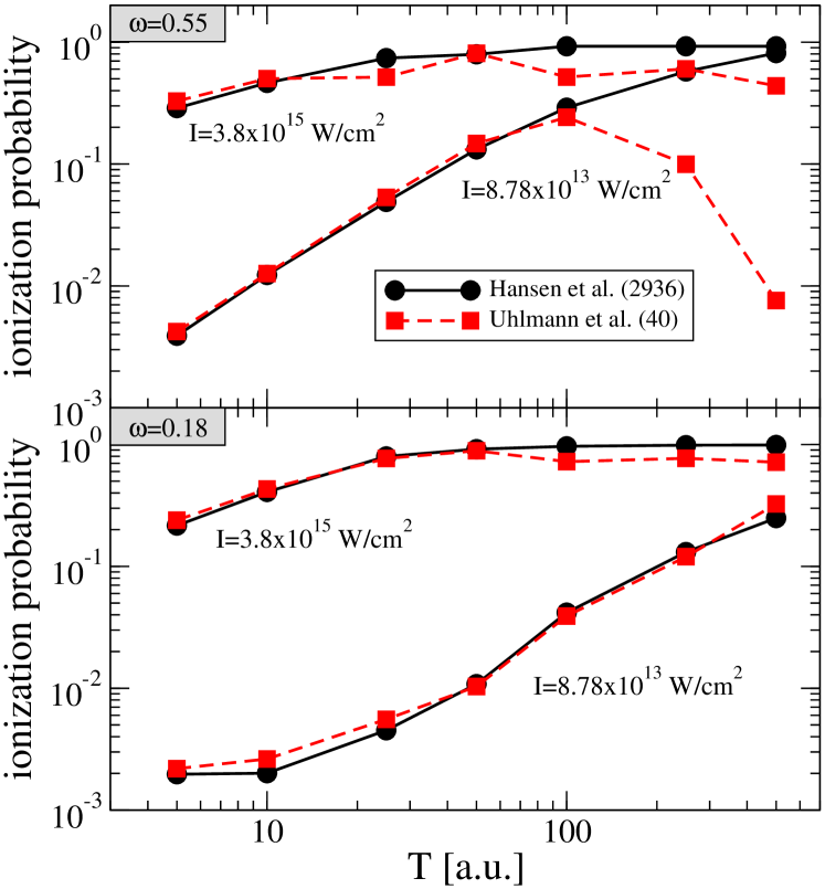
with absorber

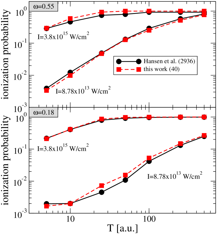
Figure 1: (Color online) The ionization probability of H(1s) as function of the laser pulse duration calculated without (left) and with (right) absorber potential. Two frequencies ($\omega=0.55$ a.u. (top) and $\omega=0.18$ a.u. (bottom)) and two laser intensities ($8.78\times 10^{13}\frac{\text{W}}{\text{cm}^{2}}$ (lower curves) and $3.8\times 10^{15}\frac{\text{W}}{\text{cm}^{2}}$ (upper curves)) have been used. Our results without absorber (Uhlmann et al. Uhlmann et al. (2005a)) and with absorber (this work) are compared to the high precision data of Hansen et al. Hansen et al. (2001). The numbers in brackets in the legends denote the size of the basis sets.

In figure 1, the ionization probabilities of H(1s) as a function of the laser pulse duration are shown. The results on the left/right side of figure 1 have been obtained in calculations without/with absorber potential. Two intensities and two wavelengths are considered. The high precision data of Hansen et al. Hansen et al. (2001) are included. As mentioned already, good agreement between our calculations without absorber and those of Hansen et al. Hansen et al. (2001) is found only if the laser pulse is relatively short or weak, i.e. if the ionization probability is small (left graphs of figure 1). The agreement for longer or more intense laser pulses is dramatically improved if the absorber is included (right graphs of figure 1).

Thus, it is possible to use a small basis set together with absorbing boundary conditions instead of an accurate treatment of the continuum. This is of special importance for molecular many-electron calculations. For these systems it is essential to use small basis sets and, thus, to introduce absorbing boundary conditions.

III.2 The molecular benchmark system: The aligned hydrogen molecular ion H${}_{2}^{+}$

Next, the absorber is tested on the molecular benchmark system, pre-aligned H${}_{2}^{+}$, i.e. the molecular axis is oriented parallel to the electric field of the laser and, thus, the nuclear motion is restricted to this axis. For this system, full quantum mechanical calculations have been performed by Chelkowski et al. Chelkowski et al. (1995) which can serve as reference calculations.

In contrast to our previous studies with a minimal Kunert and Schmidt (2003) and extended Uhlmann et al. (2003) LCAO (linear combination of atomic orbitals) basis we use here an elaborate basis set consisting of uncontracted Gaussians only (details are described in appendix B.1). It delivers an excellent description of the ground state surface with an equilibrium distance of $R_{\text{eq}}=1.9975$ a.u. and a minimum at $E_{\text{min}}=-0.60246$ a.u. (see fig. 2). The ground state energy $E_{0}=E_{\text{min}}+\frac{\omega}{2}$ and the vibrational levels $E_{n}$ ($n=1,2,\dots$) are also shown in fig. 2. They are calculated according to the Bohr-Sommerfeld formula

$$\oint p(R,E)\text{d}R=(n+n_{0})\times h$$ (42)

with $n_{0}=1/2$ for the harmonic oscillator, $n$ the vibrational quantum number, $h$ the Plancks constant and $p(R,E)$ the classical momentum as function of the energy $E$ and the distance $R$. This yields a binding energy of $E_{0}=-0.59724$ a.u., which is of quantum-chemical accuracy (cf. e.g. Yan et al. (2003)).

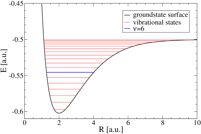
Figure 2: (Color online) Groundstate curve of H${}_{2}^{+}$ (black) and vibrational levels (thin red lines, thick blue line for $\nu=6$)

The H${}_{2}^{+}$ is now exposed to the quasi-cw laser with the parameters according to that of Chelkowski et al. Chelkowski et al. (1995). So, the laser has a short turn-on of 1 fs. The shape is kept constant afterwards. The frequency is $\omega=0.21$ a.u $=5.71$ eV and the intensity is $3.5\times 10^{13}$ W/cm². To obtain probabilities, 1000 trajectories were calculated and the results were averaged. The initial conditions of the trajectories were chosen according to the classical distance distribution in the 6th vibrationally excited state. Probabilities are defined as an average over the respective quantity for a single trajectory, i.e.

$$P_{<\text{quantity}>}=\frac{1}{n}\sum_{i=1}^{n}P_{<\text{quantity}>}^{i}\,\text{.}$$ (43)

The ionization probability for one trajectory $i$ is defined as the missing part of the norm, i.e.

$$P_{\text{ion}}^{i}(t)=1-N_{i}(t)\,\text{.}$$ (44)

The fragmentation probability is defined as

$$P_{\text{frag}}^{i}(t)=\left\{\begin{array}[]{ccc}0&\hskip 14.22636pt\text{for}&R(t)<R_{\text{D}}\\ 1&&\text{otherwise}\end{array}\right.$$ (45)

with $R_{\text{D}}=9.5$ a.u. taken from Chelkowski et al. (1995). In accordance with Chelkowski et al. a dissociation probability, i.e. fragmentation without ionization, is defined as

$$P_{\text{diss}}^{i}(t)=(1-P_{\text{ion}}^{i}(t))\,P_{\text{frag}}^{i}(t)\,\text{.}$$ (46)

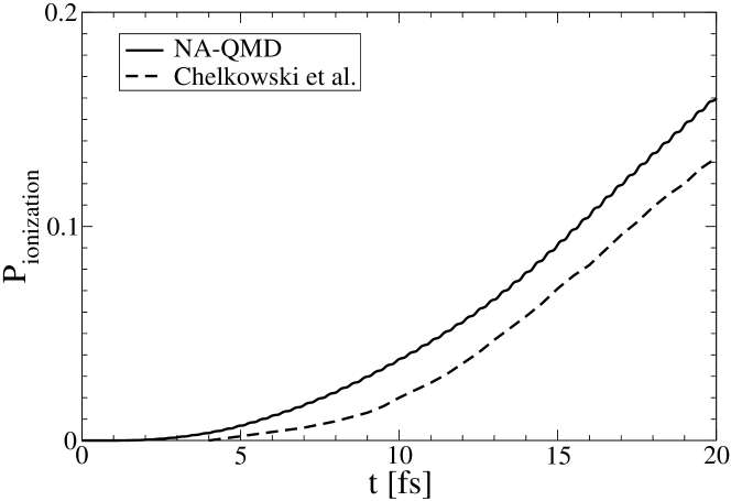
Figure 3: Ionization (top) and dissociation (bottom) probabilities of H${}_{2}^{+}$ as function of time obtained with the present NA-QMD method and by Chelkowski et al. Chelkowski et al. (1995). (see text for details)

The resulting ionization probability is shown in comparison to the full quantum mechanical results of Chelkowski et al. Chelkowski et al. (1995) in the upper part of figure 3. The present calculations result in an ionization probability that is slightly higher than the full-quantum mechanical results. This is due to the different definitions of the ionization probabilities. Whereas in grid calculations electronic density can be counted as ionized only at large distances from the center of the system (e.g. outside a cylinder with $R<32$ a.u. in Chelkowski et al. (1995)), our absorber (30) acts also in the vicinity of the nuclei. Therefore, the onset of ionization is somewhat earlier in the present calculation as compared to the results of Chelkowski et al. Chelkowski et al. (1995). After 12 fs both ionization probabilities have a nearly linear slope. Regarding the uncertainties resulting from the different definitions of absorbing boundary conditions, all in all, very good agreement between the present and the full quantum mechanical calculation is found.

In the lower part of figure 3, the associated dissociation probabilities are shown. As seen, the onset of fragmentation is slightly delayed in the NA-QMD calculations as compared to the full quantum mechanical result. This is clearly due to the classical description of the nuclei. Afterwards, the same behavior is observed, i.e. first a steep rise and after 18 fs the dissociation probability seems to run into a plateau. In spite of this qualitative agreement, the present calculation overestimates the dissociation probability by 0.08.

III.3 Non-aligned H${}_{2}^{+}$ and H₂ molecules

In this section, ionization probabilities and rates for H${}_{2}^{+}$ and H₂ are considered as function of the angle $\Theta$ between the molecular axis and the laser polarization axis as well as as function of the internuclear distance $R$ between the nuclei. Due to the lack of unaligned studies, comparison with previous work can be done only for aligned molecules, i.e. $\Theta=0$ Yu et al. (1996); Saenz (2000, 2002); Harumiya et al. (2000, 2002); Lein et al. (2002c).

All calculations have been performed with fixed nuclei. The H₂ molecule is considered in the TDHF approximation (see Kunert et al. (2005) for details). To account the orientation dependence the local basis functions centered at the nuclei are extended with functions located at hexagonal grid points (see appendix B.2 for details). With this basis the ground state surfaces exhibit equilibrium internuclear distances and energies of $R_{\text{eq}}^{H_{2}^{+}}=1.99744$ a.u., $E_{\text{min}}^{H_{2}^{+}}=-0.602455$ a.u. and $R_{\text{eq}}^{H_{2}}=1.39384$ a.u., $E_{\text{min}}^{H_{2}}=-1.13608$ a.u.

Ionization probabilities

In the following, the ionization probabilities of H${}_{2}^{+}$ and H₂ as function of $\Theta$ will be discussed. They are calculated at the equlibrium internuclear distance with a 50 fs, 266 nm and $5\times 10^{14}$ W/cm² laser pulse. For H${}_{2}^{+}$, the ionization probability $P_{\text{ion}}$ is again defined as the missing part of the norm, eq. (41). For H₂, we abbreviate the missing part of the norm of the single-particle functions with

$$P_{\text{s,}1/2}=1-N_{1/2}$$ (47)

where $N_{1/2}$ are the norms of the single-particle wave functions of the two electrons. Because both electrons differ only by their spin degrees of freedom one has of course $N_{1}=N_{2}$ and $P_{\text{s,}1}=P_{\text{s,}2}=P_{\text{s}}$. The single and double ionization probability are obtained via the single-particle approximation Lappas and van Leuwen (1998); Petersilka and Gross (1999)

$$P_{\text{single}} = (1-N_{1})N_{2}+N_{1}(1-N_{2})\,\text{,}$$ (48)

$$P_{\text{double}} = (1-N_{1})(1-N_{2})\,\text{.}$$ (49)

Note, that with the definition (48) the maximum of $P_{\text{single}}$ is $0.5$ if $N_{1}=N_{2}$.

$P_{\text{ion}}$, P${}_{\text{s}}$, $P_{\text{single}}$ and $P_{\text{double}}$ are plotted as function of the angle $\Theta$ in fig. 4. All calculated probabilities have been fitted according to

$$\Pi(\Theta)=\left(P_{\parallel}\,\cos^{2}\Theta+P_{\perp}\,\sin^{2}\Theta\right)\,\text{.}$$ (50)

This parameterization has been used by Litvinyuk et al. Litvinyuk et al. (2003) to fit their experimental data on N₂ Litvinyuk et al. (2003). The parameterization (50) fails to fit the experimental data on O₂ Alnaser et al. (2004). As can be seen from fig. 4, the parameterization (50) works very well for all probabilities in H${}_{2}^{+}$ and H₂ where experimental data do not exist to date.

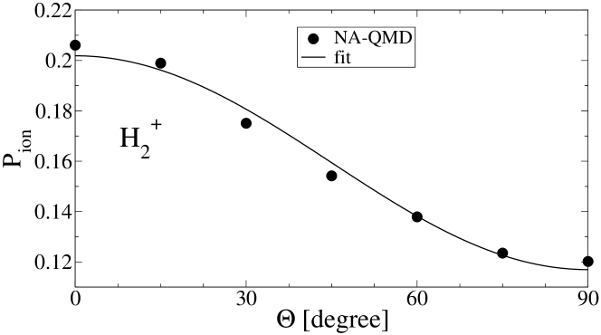
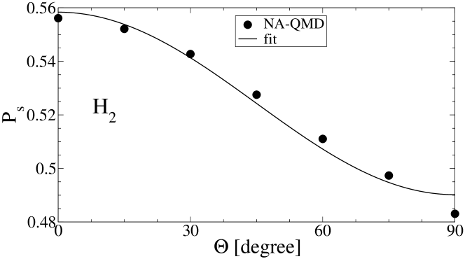
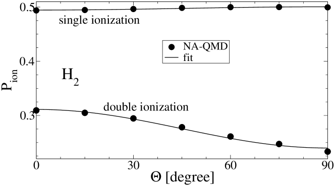
Figure 4: Ionization probabilities $P_{\text{ion}}$ for H${}_{2}^{+}$ and H₂ (top and bottom). Also, the missing part of the norm of the single-particle wave functions $P_{\text{s,}1}=P_{\text{s,}2}=P_{\text{s}}$ in H₂ is shown (middle). The symbols denote the results of the NA-QMD calculation, the full lines the $P_{\parallel}\,\cos^{2}\Theta+P_{\perp}\,\sin^{2}\Theta$ fit (see text).

From fig. 4 it becomes apparent that the probabilities $P_{\text{ion}}$ and $P_{\text{s}}$ are largest at parallel orientation $\Theta=0$ degree and decrease with increasing $\Theta$ exhibiting the minimum at perpendicular orientation $\Theta=90$ degree, for both molecules, as expected. However, the orientations dependence of the response is much more pronounced for H${}_{2}^{+}$ as compared to H₂ (note the different absolute values of the probabilities in the upper and middle part of fig. 4). In addition, the single ionization probability in H₂ is practically orientation independent, at least for the chosen laser parameters where the double ionization probability is not small (lower part of fig. 4).

Striking differences between H${}_{2}^{+}$ and H₂ have been found also in the alignment behavior of both molecules Uhlmann et al. (2005b). In a relatively large range of laser intensities, fragments originating from H${}_{2}^{+}$ are much more aligned as compared to those from H₂ Uhlmann et al. (2005b). This is in accord with the present findings of the much larger anisotropic response of H${}_{2}^{+}$ in comparison to H₂.

Ionization rates

Finally, the ionization rates $\Gamma(s^{-1})$ as function of the internuclear distance for parallel and perpendicular orientations will be considered for both molecules. They are calculated from the logarithmic decrease of the norm $N(t)$, i.e.

$$\text{ln}N(t)=-\Gamma\,t\,.$$ (51)

In the case of H₂ one has $\Gamma=\Gamma_{1}+\Gamma_{2}$ in the spirit of the independent particle model (i.e. $N(t)=N_{1}(t)\,N_{2}(t)$). The cw-laser used has a short turn-on of three optical cycles and a constant shape afterwards. The wavelength is 266 nm and different intensities have been used. For the intensity of $8\times 10^{13}$ W/cm² the resulting ionization rates as function of the internuclear distance $R$ are shown in fig. 5 for parallel and perpendicular orientation and both molecules.

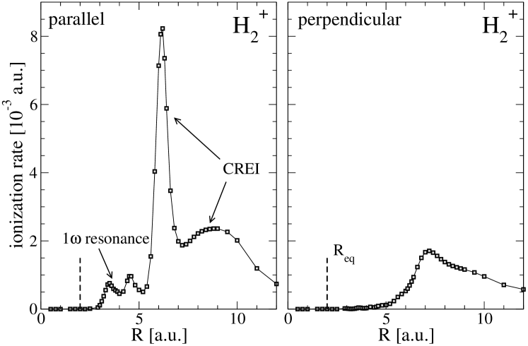
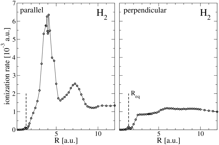
Figure 5: Ionization rates as function of the internuclear distance for H${}_{2}^{+}$ (top) and H₂ (bottom) at a laser wavelength of 266 nm and an intensity of $8\times 10^{13}$ W/cm². The vertical broken line indicates the equilibrium internuclear distance.

For H${}_{2}^{+}$ and parallel orientation (left upper part of fig. 5), the well-known features are recovered with our new formalism, i.e., enhanced ionization is observed for internuclear distances between 6 and 10 a.u. This is the well-known charge-resonance enhanced ionization (CREI) Zuo and Bandrauk (1995); Seideman et al. (1995) which is accompanied by an electron localization Seideman et al. (1995); Posthumus et al. (1995, 1996). The CREI features are observed here although the system is in the multi photon regime, i.e. the Keldysh parameter (see e.g. Dundas and Rost (2005)) is $\gamma\gg 1$. This emphasizes the generality of the CREI mechanism. At $R\approx 3.5$ a.u the one-photon resonance between the electronic groundstate and the first excited state manifests itself as a peak in the ionization rates in parallel orientation. An additional peak is found at $R\approx 4.5$ a.u. This peak is suppressed for higher intensities, for which the results are not included in figure 5.

For H₂ and parallel orientation (left lower part of fig. 5), the ionization rate exhibits two peaks which look similar to the CREI peaks of H${}_{2}^{+}$ in parallel orientation. These peaks are located at smaller internuclear distances than for H${}_{2}^{+}$. In addition, one of the peaks is split which might originate from resonances as the system is in the multiphoton regime.

The occurrence of enhanced ionization in H₂ has been also subject to a number of previous studies. First, the distance dependent ionization of H₂ was investigated using a 1D model Yu et al. (1996). Depending on laser intensity and frequency either one or two peaks were found. E.g., at $\lambda=532$ nm and $I=1\times 10^{14}$ W/cm² enhanced ionization (EI) was found at $R\approx 4$ a.u. and $R\approx 6$ a.u. which is very similar to the findings in our fully 3D calculations. The behavior of parallel aligned H₂ in static electric fields was studied with high precision quantum chemistry methods Saenz (2000, 2002), too. An avoided crossing of the H₂ groundstate and an excited state, that corresponds to the ionic fragments H⁺ and H^- in the static electric field, was found. In a fully 3D study of parallel aligned H₂ Harumiya et al. (2000, 2002) it was found as well that the enhanced ionization is linked to the formation of ionic components H⁺ and H^- as a typical signature of CREI in the H₂ molecule.

We note also, that the direct experimental observation of CREI in H${}_{2}^{+}$ has been published recently Pavičić et al. (2005). For H₂ this is not the case. Moreover, it has been shown recently in a 1D study Lein et al. (2002c) that ionization of H₂ usually takes place near the equilibrium internuclear distance. Thus, the role of the CREI mechanism in aligned H₂ remains still an open problem for future investigations.

The most surprising result of the present studies concerns the ionization probabilities in perpendicular orientation (right part of fig. 5). Clearly seen, the calculations predict enhanced ionization for both molecules. In H${}_{2}^{+}$, the ionization rate exhibits a distinct maximum at $R\approx 7$ a.u., whereas in H₂, this quantity clearly increases around $R\approx 2.5$ a.u. (Note also, that tiny peaks are found in H₂ near the equilibrium distance $R_{\text{eq}}$ for both orientations, and cf. discussion above). One can definitely exclude the CREI mechanism to be responsible for the enhanced ionization in perpendicular orientation, because electron localization cannot take place in this geometry. In H${}_{2}^{+}$, this feature probably originates from a resonance that occurs around $R\approx 7$ a.u. However, this as well as the nearly structureless enhancement of the ionization rate in H₂ remain as subjects for systematic future studies.

IV Conclusions

It was the main aim of this work to present, for the first time, a method to introduce absorbing boundary conditions in calculations of many electron systems with basis expansion. The basic idea is rather general (section II.1) and based on an imaginary potential constructed as a projection operator with time-dependent adiabatic states. In this paper it has been used to extend the NA-QMD formalism in order to describe realistically ionization processes in many electron systems.

The method was tested on the benchmark systems, the hydrogen atom and the aligned H${}_{2}^{+}$ molecule in intense laser fields. Very good agreement between the calculated ionization probabilities and that of (numerically very extensive) reference calculations has been found.

The extended NA-QMD formalism allowed us, also for the first time, to study the ionization process in unaligned H${}_{2}^{+}$ and H₂ molecules. A completely different orientation dependence of the ionization probabilities in both molecules was found, with a distinct anisotropic response in H${}_{2}^{+}$ and a nearly isotropic behavior in H₂. In addition, enhanced ionization for perpendicular orientation in both molecules is predicted, which to the best of our knowledge, has not been reported before.

The present method can be applied to larger systems, like N₂ Litvinyuk et al. (2003), O₂ Alnaser et al. (2004) or organic molecules where the experimental findings still require a consistent interpretation. Finally, we note also that the present method can also be used to study ionization processes in atomic collisions with many electrons Lüdde (2003).

Appendix A Basis transformations

In order to solve the time-dependent eigenvalue problem (29)

$$\hat{H}_{\text{eff}}^{\sigma}(t)|\chi_{a}^{\sigma}\rangle(t)=\epsilon_{a}^{\sigma}(t)|\chi_{a}^{\sigma}\rangle(t)$$ (52)

the effective single-particle “field-following” adiabatic states are expanded in the basis $\{|\phi_{\alpha}\rangle\}$ (15)

$$|\chi_{a}^{\sigma}\rangle=\sum_{\beta=1}^{N_{\text{b}}}U_{a\beta}^{\sigma}|\phi_{\beta}\rangle\,.$$ (53)

Multiplying $|\phi_{\alpha}\rangle$ with $\sum_{a}|\chi_{a}^{\sigma}\rangle\langle\chi_{a}^{\sigma}|$ the expansion of $|\phi_{\alpha}\rangle$ in the basis $\{|\chi_{a}^{\sigma}\rangle\}$ results

$$|\phi_{\alpha}\rangle=\sum_{a\beta}^{N_{\text{b}}}S_{\alpha\beta}U_{\beta a}^{\sigma+}|\chi_{a}^{\sigma}\rangle\,.$$ (54)

Note, that $\sum_{a}|\chi_{a}^{\sigma}\rangle\langle\chi_{a}^{\sigma}|$ can be used like an identity because the basis sets $\{|\phi_{\alpha}\rangle\}$ and $\{|\chi_{a}\rangle\}$ span exactly the same part of the Hilbert space. Furthermore, the property

$$\sum_{a=1}^{N_{\text{b}}}U_{\beta a}^{\sigma+}U_{a\gamma}^{\sigma}=\left(S^{-1}\right)_{{\beta\gamma}}$$ (55)

is obtained by using (53) and (54). Therefore, the transformation $\hat{U}^{\sigma}$ is unitary only if both basis sets are orthogonal, i.e. if also $\left(S^{-1}\right)_{{\beta\gamma}}=\delta_{\beta\gamma}$.

Inserting (53) into (52) and multiplying with $\langle\phi_{\alpha}|$ results in the generalized eigenvalue problem

$$\sum_{\beta=1}^{N_{\text{b}}}\left(\langle\phi_{\alpha}|\hat{H}_{\text{eff}}^{\sigma}|\phi_{\beta}\rangle-\epsilon_{a}^{\sigma}\langle\phi_{\alpha}|\phi_{\beta}\rangle\right)U_{a\beta}^{\sigma}=0\,.$$ (56)

The effective single-particle energies $\epsilon_{a}^{\sigma}$ and the transformation $\hat{U}^{\sigma}$ are obtained by solving (56).

The effective single-particle wave function $|\Psi^{j\sigma}\rangle$ (15) can either be expanded in the basis $\{|\phi_{\alpha}\rangle\}$ or in the basis $\{|\chi_{a}\rangle\}$

$$|\Psi^{j\sigma}\rangle(t)=\sum_{\alpha=1}^{N_{\text{b}}}a^{j\sigma}_{\alpha}(t)|\phi_{\alpha}\rangle(t))=\sum_{a=1}^{N_{\text{b}}}a^{j\sigma}_{a}(t)|\chi_{a}\rangle(t))\hskip 28.45274pt\text{with}\hskip 14.22636ptj=1\dots N_{\text{e}}^{\sigma},\,\sigma=\uparrow,\downarrow\,.$$ (57)

Using equations (53) and (57) the transformations for the coefficients $a_{\alpha}^{j\sigma}$ and $a_{a}^{j\sigma}$

$$a_{a}^{j\sigma} = \langle\chi_{a}^{\sigma}|\Psi^{j\sigma}\rangle=\sum_{\alpha\beta}^{N_{\text{b}}}U_{\alpha a}^{\sigma+}a_{\beta}^{j\sigma}S_{\alpha\beta}\,,$$ (58)

$$a_{\alpha}^{j\sigma} = \sum_{a=1}^{N_{\text{b}}}U_{a\alpha}^{\sigma}a_{a}^{j\sigma}$$ (59)

and a general matrix $O_{\alpha\beta}^{\sigma}$ and $O_{ab}^{\sigma}$

$$O_{ab}^{\sigma} = \langle\chi_{a}|\hat{O}|\chi_{b}\rangle=\sum_{\alpha\beta}^{N_{\text{b}}}U_{\alpha a}^{\sigma+}O_{\alpha\beta}^{\sigma}U_{b\beta}^{\sigma}\,,$$ (60)

$$O_{\alpha\beta}^{\sigma} = \langle\phi_{\alpha}|\hat{O}|\phi_{\beta}\rangle=\sum_{ab\gamma\delta}^{N_{\text{b}}}S_{\alpha\gamma}U_{a\gamma}^{\sigma}O_{ab}^{\sigma}U_{\delta b}^{\sigma+}S_{\delta\beta}$$ (61)

are obtained. The last transformation is used to calculate the matrix elements $V_{\text{abs, }{\alpha\beta}}^{\sigma}$ which are used in practical calculations.

Appendix B Basis sets

In this appendix all details of the basis sets used in the H${}_{2}^{+}$ and H₂ calculations are given to make the calculations comprehensible. The basis set used in the H calculations (section III.1) consists of the hydrogen 1s, 2s and 2p${}_{\text{z}}$ basis functions extended with chains of s-type Gaussians and is described in detail in Uhlmann et al. (2005a).

B.1 Aligned H${}_{2}^{+}$

The basis set that is used in the calculations to aligned H${}_{2}^{+}$ (section III.2) is a combination of a local basis centered at each of the two nuclei and a chain of additional s-type Gaussians located along the laser polarization axis. Gaussians

$$\phi_{Ailm}(\vec{r}\,^{\prime})=N\,Y_{lm}(\theta^{\prime},\phi^{\prime})\,\text{e}^{-\frac{r_{\text{A}}^{2}}{\sigma_{i}^{2}}}$$ (62)

are used also as basis functions at the nuclei. In (62) $Y_{lm}$ are the spherical harmonics, $N$ is a norm constant, $\sigma_{i}$, $l$ and $m$ are parameters of the basis functions and $\vec{r}_{\text{A}}=\vec{r}-\vec{R}_{A}$ where $\vec{R}_{A}$ is the center of the basis function (see e.g. Kunert (2003)). At each of the two nuclei a basis set that consists of such Gaussians is located. The $\sigma_{i}$ are determined with

$$\sigma_{i}=\sigma_{1}\,f^{i-1}\hskip 56.9055pt(1\leq i\leq N)\,$$ (63)

where $\sigma_{1}$, $f$, $N$ are parameters given in table 1. With this basis set the atomic as well as the molecular groundstate are described extremely well. Furthermore, a good description of the excited states of H${}_{2}^{+}$ is achieved with this basis set. Please note, that the $\sigma_{1}$ for $l=1$ and $l=2$ have been chosen in such a way that $\sigma_{\text{max}}^{l=2}=1.7^{1/3}\,\sigma_{\text{max}}^{l=1}=1.7^{2/3}\,\sigma_{\text{max}}^{l=0}$.

l	f	$\sigma_{1}$ [a.u.]	$\sigma_{\text{max}}$ [a.u.]	N
0	1.7	0.05	3.487	9
1	1.7	0.8473	4.162	4
2	1.7	1.7191	4.968	3

Table 1: Gaussian basis centered at each of the protons of H${}_{2}^{+}$. The parameters given are those of equation (63).

The parameters of the additional chain of s-type Gaussians (see e.g. Uhlmann et al. (2005a); Uhlmann et al. (2003)) that is laid out symmetrically to the origin along the $z$-axis are given in table 2. These additional functions have nearly no influence on the already excellent description of the groundstate and the lowest excited states. They do, however, improve the description of highly excited and ionized electronic states and a dense level structure around $E=0$ results. The parameters given in table  2 were determined using the formalism described in Uhlmann et al. (2005a).

$\sigma$ [a.u.]	$d$ [a.u.]	$n$
5.54	3.7	21

Table 2: Parameters of the chain (width $\sigma$, spacing $d$ between neighboring functions and number $n$ of functions) of s-type Gaussians laid out symmetrically to the origin along the $z$ axis.

B.2 Unaligned H${}_{2}^{+}$ and H₂

The same basis as before (see table 1) is located at each of the hydrogen atoms in the calculations to unaligned H${}_{2}^{+}$ and H₂ (section III.3). However, a hexagonal grid of additional basis functions in the $y$-$z$ plane

$$\left(\begin{array}[]{c}x_{ij}\\ y_{ij}\\ z_{ij}\end{array}\right)=\left(\begin{array}[]{c}0\\ \left(i-\frac{N_{1}}{2}\right)\frac{d}{2}\\ \left(j-\frac{N_{2}}{2}\right)\sqrt{3}d+\left|\left(i-\frac{N_{1}}{2}\right)\text{mod}2\right|\frac{\sqrt{3}}{2}d\end{array}\right)$$ (64)

with

$$0\leq i<N_{1}$$ and

$$0\leq j<N_{2}-1 \hskip 5.69046pt\text{if }N_{1}+i\text{ even}$$ or

$$0\leq j<N_{2} \hskip 5.69046pt\text{if }N_{1}+i\text{ odd}$$

is used to extend the basis sets at the nuclei instead of the chain of Gaussians described in appendix B.1. It is thus possible to calculate the response of unaligned molecules to the laser field. The parameters of the two hexagonal grids and the one chain are given in table 3 and were also determined using the formalism described in Uhlmann et al. (2005a). The last set of Gaussians positioned at different places in space has such a large width and therefore also a large spacing that it is not necessary to build a hexagonal grid for these Gaussians. Instead these basis functions are again laid out chain-like along the $z$ axis Uhlmann et al. (2003).

$\sigma$ [a.u.]	d [a.u.]	$N_{1}$	$N_{2}$
5.74	5.2	9	7
7.81	10.38	5	3
16.62	18.68	-	3

Table 3: Parameters of the hexagonal grids (first two lines) and chain (bottom line) of s-type Gaussians laid out in the $y$-$z$ plane.

It is reasonable to use a basis set for the density in the H₂ calculations. The “exact” density, i.e. the sum over the absolute square of the single-particle functions, is expanded in this density basis to accelerate the calculation of Coulomb and xc matrix elements. Please note, that the norm of the density basis functions is different from the usual L₂(R³) norm (see Kunert (2003)). The parameters of the density basis used in the H₂ calculations are given in table 4. $\sigma_{1}=0.05/\sqrt{2}$ has been chosen because the multiplication of two Gaussians with the width $0.05$ at the same place results in a Gaussian with a width $0.05/\sqrt{2}$. This density basis had not been transformed, i.e. the uncontracted Gaussians were used.

l	f	$\sigma_{1}$ [a.u.]	$\sigma_{\text{max}}$ [a.u.]	N
0	1.7	$\frac{0.05}{\sqrt{2}}=0.035355339$	2.46	9

Table 4: Gaussian basis used as the H density basis. The parameters given are those of equation (63).

Density basis functions are also located at the additional centers specified in table 3. The $\sigma_{\text{dens}}$ of the density basis functions are set to $\sigma/\sqrt{2}$.

References

- McPherson et al. (1987) A. McPherson, G. Gibson, H. Jara, U. Johann, T. S. Luk, I. McIntyre, K. Boyer, and C. K. Rhodes, J. Opt. Soc. Am. B 4, 595 (1987).
- Ferray et al. (1988) M. Ferray, A. L’Huillier, X. F. Li, L. A. Lompré, G. Mainfray, and C. Manus, J. Phys. B 21, L31 (1988).
- Li et al. (1989) X. F. Li, A. L’Huillier, M. Ferray, L. A. Lompré, and G. Mainfray, Phys. Rev. A 39, 5751 (1989).
- Agostini et al. (1979) P. Agostini, F. Fabre, G. Mainfray, G. Petite, and N. K. Rahman, Phys. Rev. Lett. 42, 1127 (1979).
- Kruit et al. (1983) P. Kruit, J. Kimman, H. G. Muller, and M. J. van der Wiel, Phys. Rev. A 28, 248 (1983).
- Fedorov (1997) M. V. Fedorov, Atomic And Free Electrons In A Strong Light Field (World Scientific, Singapore, 1997).
- Pont and Gavrila (1990) M. Pont and M. Gavrila, Phys. Rev. Lett. 65, 2362 (1990).
- de Boer et al. (1993) M. P. de Boer, J. H. Hoogenraad, R. B. Vrijen, L. D. Noordam, and H. G. Muller, Phys. Rev. Lett. 71, 3263 (1993).
- de Boer et al. (1994) M. P. de Boer, J. H. Hoogenraad, R. B. Vrijen, R. C. Constantinescu, L. D. Noordam, and H. G. Muller, Phys. Rev. A 50, 4085 (1994).
- Yuan and George (1978) M. Yuan and T. S. George, J. Chem. Phys. 68, 3040 (1978).
- Bandrauk and Sink (1981) A. D. Bandrauk and M. L. Sink, J. Chem. Phys. 74, 1110 (1981).
- Posthumus et al. (2000) J. H. Posthumus, J. Plumridge, L. J. Frasinski, K. Codling, E. J. Divall, A. J. Langley, and P. F. Taday, J. Phys. B 33, L563 (2000).
- Yao and Chu (1993) G. Yao and S.-I. Chu, Phys. Rev. A 48, 485 (1993).
- Charron et al. (1993) E. Charron, A. Giusti-Suzor, and F. H. Mies, Phys. Rev. Lett. 71, 692 (1993).
- Giusti-Suzor et al. (1995) A. Giusti-Suzor, F. H. Mies, L. F. DiMauro, E. Charron, and B. Yang, J. Phys. B 28, 309 (1995).
- Sändig et al. (2000) K. Sändig, H. Figger, and T. W. Hänsch, Phys. Rev. Lett. 85, 4876 (2000).
- Williams et al. (2000) I. D. Williams, P. McKenna, B. Srigengan, I. M. G. Johnson, W. A. Bryan, J. H. Sanderson, A. El-Zein, T. R. J. Goodworth, W. R. Newell, P. F. Taday, et al., J. Phys. B 33, 2743 (2000).
- Giusti-Suzor et al. (1990) A. Giusti-Suzor, X. He, O. Atabek, and F. H. Mies, Phys. Rev. Lett. 64, 515 (1990).
- Bucksbaum et al. (1990) P. H. Bucksbaum, A. Zavriyev, H. G. Muller, and D. W. Schumacher, Phys. Rev. Lett. 64, 1883 (1990).
- Codling and Frasinski (1993) K. Codling and L. J. Frasinski, J. Phys. B 26, 783 (1993).
- Zuo and Bandrauk (1995) T. Zuo and A. D. Bandrauk, Phys. Rev. A 52, R2511 (1995).
- Seideman et al. (1995) T. Seideman, M. Y. Ivanov, and P. B. Corkum, Phys. Rev. Lett. 75, 2819 (1995).
- Yu and Bandrauk (1995) H. Yu and A. D. Bandrauk, J. Chem. Phys. 102, 1257 (1995).
- Kopold et al. (1998) R. Kopold, W. Becker, and M. Kleber, Phys. Rev. A 58, 4022 (1998).
- Lappas and Marangos (2000) D. G. Lappas and J. P. Marangos, J. Phys. B 33, 4679 (2000).
- Lein et al. (2002a) M. Lein, N. Hay, R. Velotta, J. P. Marangos, and P. L. Knight, Phys. Rev. Lett. 88, 183903 (2002a).
- Lein et al. (2002b) M. Lein, N. Hay, R. Velotta, J. P. Marangos, and P. L. Knight, Phys. Rev. A 66, 023805 (2002b).
- Lein et al. (2003) M. Lein, P. P. Corso, J. P. Marangos, and P. L. Knight, Phys. Rev. A 67, 023819 (2003).
- Kamta and Bandrauk (2004) G. L. Kamta and A. D. Bandrauk, Phys. Rev. A 70, 011404(R) (2004).
- Zimmermann et al. (2005) B. Zimmermann, M. Lein, and J. M. Rost, Phys. Rev. A 71, 033401 (2005).
- Chirilă and Lein (2005) C. C. Chirilă and M. Lein, J. Mod. Opt. (2005), accepted, http://www.mpi-hd.mpg.de/keitel/mlein/papers/Chirila_Lein.pdf.
- Litvinyuk et al. (2003) I. V. Litvinyuk, K. F. Lee, P. W. Dooley, D. M. Rayner, D. M. Villeneuve, and P. B. Corkum, Phys. Rev. Lett. 90, 233003 (2003).
- Alnaser et al. (2004) A. S. Alnaser, S. Voss, X.-M. Tong, C. M. Maharjan, P. Ranitovic, B. Ulrich, T. Osipov, B. Shan, Z. Chang, and C. L. Cocke, Phys. Rev. Lett. 93, 113003 (2004).
- Zhao et al. (2003) Z. X. Zhao, X. M. Tong, and C. D. Lin, Phys. Rev. A 67, 043404 (2003).
- Talebpour et al. (1998) A. Talebpour, S. Larochelle, and S. L. Chin, J. Phys. B 31, 2769 (1998).
- Wells et al. (2002) E. Wells, M. J. DeWitt, and R. R. Jones, Phys. Rev. A 66, 013409 (2002).
- Talebpour et al. (1996) A. Talebpour, C. Y. Chien, and S. L. Chin, J. Phys. B 29, L677 (1996).
- Guo et al. (1998) C. Guo, M. Li, J. P. Nibarger, and G. N. Gibson, Phys. Rev. A 58, R4271 (1998).
- DeWitt et al. (2001) M. J. DeWitt, E. Wells, and R. R. Jones, Phys. Rev. Lett. 87, 153001 (2001).
- Faisal et al. (1999) F. H. M. Faisal, A. Becker, and J. Muth-Böhm, Laser Physics 9, 115 (1999).
- Muth-Böhm et al. (2000) J. Muth-Böhm, A. Becker, and F. H. M. Faisal, Phys. Rev. Lett. 85, 2280 (2000).
- Kjeldsen and Madsen (2004) T. K. Kjeldsen and L. B. Madsen, J. Phys. B 37, 2033 (2004).
- Dundas and Rost (2005) D. Dundas and J. M. Rost, Phys. Rev. A 71, 013421 (2005).
- Geltman (2000) S. Geltman, J. Phys. B 33, 1967 (2000).
- Hansen et al. (2001) J. P. Hansen, J. Lu, L. B. Madsen, and H. M. Nilsen, Phys. Rev. A 64, 033418 (2001).
- Dundas et al. (1999) D. Dundas, K. T. Taylor, J. S. Parker, and E. S. Smyth, J. Phys. B 32, L231 (1999).
- Parker et al. (2000) J. S. Parker, L. R. Moore, D. Dundas, and K. T. Taylor, J. Phys. B 33, L691 (2000).
- Chelkowski et al. (1995) S. Chelkowski, T. Zuo, O. Atabek, and A. D. Bandrauk, Phys. Rev. A 52, 2977 (1995).
- Harumiya et al. (2000) K. Harumiya, I. Kawata, H. Kono, and Y. Fujimura, J. Chem. Phys. 113, 8953 (2000).
- Harumiya et al. (2002) K. Harumiya, H. Kono, Y. Fujimura, I. Kawata, and A. D. Bandrauk, Phys. Rev. A 66, 043403 (2002).
- Runge and Gross (1984) E. Runge and E. K. U. Gross, Phys. Rev. Lett. 52, 997 (1984).
- Saalmann and Schmidt (1996) U. Saalmann and R. Schmidt, Z. Phys. D 38, 153 (1996).
- Kunert and Schmidt (2003) T. Kunert and R. Schmidt, Eur. Phys. J. D 25, 15 (2003).
- Uhlmann et al. (2003) M. Uhlmann, T. Kunert, F. Grossmann, and R. Schmidt, Phys. Rev. A 67, 013413 (2003).
- Calvayrac et al. (1998) F. Calvayrac, P. G. Reinhard, and E. Suraud, J. Phys. B 31, 5023 (1998).
- Suraud and Reinhard (2000) E. Suraud and P. G. Reinhard, Phys. Rev. Lett. 85, 2296 (2000).
- Calvayrac et al. (2000) F. Calvayrac, P. G. Reinhard, E. Suraud, and C. Ullrich, Phys. Rep. 337, 493 (2000).
- Dundas (2004) D. Dundas, J. Phys. B. 37, 2883 (2004).
- Castro et al. (2004) A. Castro, M. A. L. Marques, J. A. Alonso, G. F. Bertsch, and A. Rubio, Eur. Phys. J. D 28, 211 (2004).
- Saalmann and Schmidt (1998) U. Saalmann and R. Schmidt, Phys. Rev. Lett. 80, 3213 (1998).
- Kunert and Schmidt (2001) T. Kunert and R. Schmidt, Phys. Rev. Lett. 86, 5258 (2001), and refs therein.
- Kunert et al. (2005) T. Kunert, F. Grossmann, and R. Schmidt, Phys. Rev. A 72, 023422 (2005).
- Uhlmann et al. (2005a) M. Uhlmann, T. Kunert, and R. Schmidt, Phys. Rev. E 72 (2005a), in print.
- Kono et al. (2003) H. Kono, Y. Sato, Y. Fujimura, and I. Kawata, Las. Phys. 13, 883 (2003).
- Kono et al. (2004) H. Kono, Y. Sato, N. Tanaka, T. Kato, K. Nakai, S. Koseki, and Y. Fujimura, Chem. Phys. 304, 203 (2004).
- Neuhasuer and Baer (1989) D. Neuhasuer and M. Baer, J. Chem. Phys. 90, 4351 (1989).
- Dundas et al. (2000) D. Dundas, J. F. McCann, J. S. Parker, and K. T. Taylor, J. Phys. B 33, 3261 (2000).
- (68) D. Dundas, private communication.
- Yan et al. (2003) Z.-C. Yan, J.-Y. Zhang, and Y. Li, Phys. Rev. A 67, 062504 (2003).
- Yu et al. (1996) H. Yu, T. Zuo, and A. D. Bandrauk, Phys. Rev. A 54, 3290 (1996).
- Saenz (2000) A. Saenz, Phys. Rev. A 61, 051402(R) (2000).
- Saenz (2002) A. Saenz, Phys. Rev. A 66, 063407 (2002).
- Lein et al. (2002c) M. Lein, T. Kreibich, E. K. U. Gross, and V. Engel, Phys. Rev. A 65, 033403 (2002c).
- Lappas and van Leuwen (1998) D. Lappas and R. van Leuwen, J. Phys. B 31, L249 (1998).
- Petersilka and Gross (1999) M. Petersilka and E. K. U. Gross, Laser Physics 9, 105 (1999).
- Uhlmann et al. (2005b) M. Uhlmann, T. Kunert, and R. Schmidt, Phys. Rev. A (2005b), accepted.
- Posthumus et al. (1995) J. H. Posthumus, L. J. Frasinski, A. J. Giles, and K. Codling, J. Phys. B 28, L349 (1995).
- Posthumus et al. (1996) J. H. Posthumus, A. J. Giles, M. R. Thompson, and K. Codling, J. Phys. B 29, 5811 (1996).
- Pavičić et al. (2005) D. Pavičić, A. Kiess, T. W. Hänsch, and H. Figger, Phys. Rev. Lett. 94, 163002 (2005).
- Lüdde (2003) H. J. Lüdde, Time-Dependent Density Functional Theory in Atomic Collisions in: Many-Particle Quantum Dynamics in Atomic and Molecular Fragmentation (Springer, 2003), chap. 12.
- Kunert (2003) T. Kunert, Ph.D. thesis, Technische Universität Dresden (2003).