Coherent Backscattering of Light with Nonlinear Atomic Scatterers

Abstract

We study coherent backscattering of a monochromatic laser by a dilute gas of cold two-level atoms in the weakly nonlinear regime. The nonlinear response of the atoms results in a modification of both the average field propagation (nonlinear refractive index) and the scattering events. Using a perturbative approach, the nonlinear effects arise from inelastic two-photon scattering processes. We present a detailed diagrammatic derivation of the elastic and inelastic components of the backscattering signal both for scalar and vectorial photons. Especially, we show that the coherent backscattering phenomenon originates in some cases from the interference between three different scattering amplitudes. This is in marked contrast with the linear regime where it is due to the interference between two different scattering amplitudes. In particular we show that, if elastically scattered photons are filtered out from the photo-detection signal, the nonlinear backscattering enhancement factor exceeds the linear barrier two, consistently with a three-amplitude interference effect.

I Introduction

Propagation of light waves in disordered media is an active research area since hundred years ago now. The original scientific motivation came from astrophysical questions about properties of light radiated by interstellar atmospheres schuster ; mihalas . Then, within the first decades of the twentieth century, the foundations of light transport in this regime were laid, leading to the radiative transfer equations chandra ; hulst ; holstein ; molisch . The basic physical ingredient of these equations is a detailed analysis of energy transfers (scattering, absorption, sources, etc). Sufficiently far from any boundaries, the long-time and large spatial scale limits of these equations give rise, in the simplest cases, to a physically appealing diffusion equation.

One important feature of this theory is to consider that any possible interference effects are washed out under disorder average. This is a random-phase assumption. For a long time, it was believed that this was still the case on average for monochromatic light elastically scattered off an optically thick sample even if, for a given disorder realization, one observes a speckle pattern dainty indicating that phase coherence is preserved by the scattering process. Theoretical and experimental works in electronic transport anderson ; langer ; bergmann made soon clear that this random-phase assumption was wrong in the elastic regime. Depending on the disorder strength, partial (weak localization regime) or complete (strong localization regime) suppression of diffusive behavior has been predicted, provided phase coherence is preserved over a sufficient large number of scattering events houches ; akkermon . In turn, these discoveries have cross-fertilized the field of light transport in the elastic regime photon ; ucf ; locaforte ; dws . In this field, one of the hallmark of interference effects in elastic transport is the coherent backscattering (CBS) phenomenon cbs ; cbsdiffusion : the average intensity multiply scattered off an optically thick sample is larger than the average background in a small angular range around the direction opposite to the ingoing light. This interference enhancement of the diffuse reflection off the sample is a manifestation of a two-wave interference. As such, it probes the coherence properties of the outgoing light and it has been extensively studied both experimentally and theoretically. It can be shown on general arguments, that the CBS enhancement factor (defined as the ratio of the backscattering CBS peak to diffuse background) never exceeds the value 2 and is obtained in the helicity-preserving polarization channel for scatterers with spherical symmetry bvtmaynard .

Whereas these interference modifications of transport are by now widely understood in the case of linear media, recent experimental developments have required an extension of multiple scattering theory to the nonlinear case. Even if few studies already exists, they only cover the simpler case of classical linear scatterers embedded in a nonlinear medium cbsnl1 ; cbsnl2 , whereas in our microscopic approach, the nonlinear behavior of randomly distributed scatterers will affect both the scattering processes and the average propagation. In particular, with the advent of laser cooling, on the one hand, it has become possible to study interference effects in multiple scattering of light by cold atoms labeyrie99 ; jonckheere00 ; cord1 ; cord2 ; havey1 . In the regime where the saturation of the atomic transition sets in, atoms scatter light nonlinearly, i.e. the scattered light is no longer proportional to the incident one. One should note that important nonlinear effects are easily achieved with atoms even at moderate laser intensities. Considering a given driven optical dipole atomic transition, the order of magnitude of the required light intensity to induce nonlinear effects is given by the so-called saturation intensity $I_{s}$ and is generally low. As typical examples, it is 1.6 mW/cm² for Rubidium atoms and 42 mW/cm² for Strontium atoms, for their usual laser cooling transitions. On the other hand, random lasers - mirrorless lasers where feedback is provided by multiple scattering lethokov - have been realized experimentally lawandy94 ; cao99 . Here, nonlinear effects occur in the regime close to or above the laser threshold. Since, at least in the regime of coherent feedback cao , interference is believed to play a decisive role in the physics of the random laser, a better understanding of the influence of nonlinearity (and amplification) on the properties of coherent wave transport becomes necessary.

II Motivation and outline

In a recent contribution wellens2 , we have shown that nonlinear scattering may fundamentally affect interference in multiple scattering. Indeed, in the perturbative regime of at most one scattering event with $\chi^{(3)}$ nonlinearity, there are now three (and no longer two) CBS interfering amplitudes. Depending on the sign of the nonlinearity, i.e. depending whether nonlinear effects enhance or decrease the scattering cross section, the effect of this three-wave interference effect leads to a significant increase or decrease of the nonlinear CBS enhancement factor.

The purpose of the present paper is, on the one hand, to provide a detailed derivation of the equations for the nonlinear coherent backscattering signal used in wellens2 , and, on the other one, to extend the treatment of wellens2 to the case of atomic scatterers. Here, in contrast to the classical case, light is scattered inelastically, i.e. the scattered photons may change their frequencies. This leads to dephasing between interfering amplitudes and, consequently, to a reduction of the CBS enhancement factor in addition to the nonlinear modifications mentioned above. Theoretical studies of this inelastic decoherence mechanism have been so far restricted to the case of two atoms wellens ; slava ; langevin . Since the total (linear and nonlinear) elastic signal can be filtered out by means of a suitable frequency-selective detection, a clear experimental study of inelastic, nonlinear CBS becomes possible. Please note that this would be otherwise very difficult to achieve since for weak intensities - the regime where our theory is valid - the linear signal generally largely dominates over the nonlinear one. In this paper, we will show that the enhancement factor for inelastically scattered light significantly exceeds the linear barrier two in certain frequency windows. In contrast, the total enhancement factor - including also elastically scattered light - is diminished by nonlinear scattering. This is due to the negative sign of the total nonlinear component, since the total (elastic plus inelastic) scattering cross section is decreased by saturation.

The paper is organized as follows. In Sec. III, we present the perturbative theory for nonlinear CBS of light scattered off a sample of cold two-level atoms. ‘Perturbative’ here means that we restrict ourselves to the regime of scalar - i.e., we forget the polarization of the photon - two-photon scattering with at most one nonlinear scattering event. This assumption is valid at sufficiently low probe intensities and not too large optical thicknesses. After shortly sketching the main results of the linear case, Sec. III.1, we derive equations for the nonlinear backscattering signal in Sec. III.2. The latter contains an inelastic and an elastic component. The latter again splits into a nonlinear and a linear part. In Sec. III.3, supplemented by appendix A, we show how to generalize our scalar theory to the vectorial case by explicitly taking into account the light polarization degrees of freedom. It is shown that nonlinear polarization effects lead to decoherence between interfering paths. In contrast to the linear case, this decoherence mechanism cannot be avoided by a suitable choice of the polarization detection channel. In order to emphasize the generality of our approach, we shortly discuss in Sec. III.4 a model of classical, nonlinear scatterers, which reproduces the elastic backscattering signal of the atomic model. In Sec. IV, we apply our theory to the case of a disordered atomic medium with slab geometry. We look at the dependence of the backscattering signal as a function of the optical thickness and of the detuning of the laser from the atomic resonance. In particular, we show that the enhancement factor for the inelastic component significantly exceeds the linear barrier two in certain frequency windows. Finally, Sec. V concludes the paper.

III Theory

In this section, we present the perturbative theory for nonlinear coherent backscattering of light from a gas of cold two-level atoms. We first treat the linear component of the backscattering signal, which results from scattering of independent photons. Thereby we introduce the reader, in Sec. III.1, to standard methods used in linear multiple scattering theory multiple , which we will then generalize to the non-linear case in Sec. III.2.

III.1 Scalar linear regime

III.1.1 One-photon scattering amplitude

By definition, the linear component of the photo-detection signal is proportional to the incoming intensity, in particular to the number of photons in the initial laser mode. Since this implies that the photons are independent from each other, it is sufficient to know how a single photon propagates in the atomic medium, see Fig. 1. This is equivalent to using the usual Maxwell’s equations for a disordered medium multiple .

In the weak scattering regime, which we will consider throughout this paper, transport is depicted as a succession of propagation in an average medium interrupted by scattering events. The important building block to properly describe scattering and average propagation is the one-photon scattering amplitude by a single atom. For near-resonant scattering, and for atoms with no ground-state internal Zeeman degeneracies, it reads :

$$S_{\omega}=\frac{-4\pi i}{k(1-2i\delta/\Gamma)}.$$ (1)

It can be derived from the elastically-bound electron model in the limit of small light detuning $\delta=\omega-\omega_{\rm at}\ll\omega,\omega_{\rm at}$ multiple . The atomic angular transition frequency is $\omega_{\rm at}$ whereas the atomic transition width $\Gamma$ describes radiative decay. The photon wave number is $k$ and the photon angular frequency is $\omega=ck$ ($c$ being the vacuum speed of light).

For simplicity, we work here with scalar photons, i.e. we discard the vectorial nature of the light field. Scattering is then fully isotropic and the differential scattering cross-section simply reads

$$\frac{\mathrm{d}\sigma}{\mathrm{d}\Omega}=\left|\frac{S_{\omega}}{4\pi}\right|^{2}=\frac{\sigma}{4\pi}$$ (2)

leading to

$$\sigma=\frac{\sigma_{0}}{1+(2\delta/\Gamma)^{2}}\qquad;\qquad\sigma_{0}=\frac{4\pi}{k^{2}}$$ (3)

where $\sigma_{0}$ is the on-resonance scattering cross-section.

The scalar assumption is not a crucial one: as will be shown in Sec. III.3, the following treatment can be generalized to the vectorial case. Please note however that the inclusion of internal degeneracies is not immediately simple and requires a separate treatment on its own. This is so because then the internal dynamics is no longer simple (optical pumping sets in). In this respect the results presented throughout this paper only apply to non-degenerate ground-state atoms. Please note also that internal degeneracies are already known to strongly reduce the CBS effect in the linear regime cord1 ; cord2 .

III.1.2 Linear refraction index

Between two successive scattering events occurring at ${\bf r}$ and ${\bf r^{\prime}}$, the photon experiences an effective atomic medium with refractive index $n_{\omega}$. Formally, the resulting propagation is described by the average Green’s function:

$$G_{\omega}({\bf r},{\bf r^{\prime}})=-\frac{e^{in_{\omega}k|{\bf r}-{\bf r^{\prime}}|}}{4\pi\,|{\bf r}-{\bf r^{\prime}}|},$$ (4)

where the refractive index is given by index :

$$n_{\omega}=1-\frac{\delta}{\Gamma k\ell}+\frac{i}{2k\ell}.$$ (5)

The imaginary part of $n_{\omega}$ describes depletion by scattering. This depletion gives rise to the exponential attenuation of the direct transmission through the sample (Beer-Lambert law) and defines, via the optical theorem, the linear mean-free path at frequency $\omega$ as

$$\ell=\frac{1}{{\mathcal{N}}\sigma}$$ (6)

where $\mathcal{N}$ denotes the density number of atoms in the sample. The weak scattering condition, where all the previous (and following) results are valid, then simply reads $k\ell\gg 1$.

III.1.3 Linear radiative transfer equation

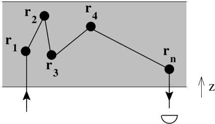
Figure 1: Scattering path of a single photon entering the medium and leaving it in the backscattering direction to reach the detector. Straight lines depict average propagation in the effective medium while full circles depict scattering events labeled by the $\textbf{r}_{n}$.

We have now at hand all the necessary ingredients to write down the amplitude of a multiple scattering process as the one sketched in Fig. 1. We consider a scattering volume $V$ exposed to an initial monochromatic field with amplitude $E_{0}$ propagating along axis $z$. The transverse area of the scattering volume is $\Sigma$. Since $k\ell\gg 1$, a semi-classical picture using well-defined scattering paths is appropriate. For a given scattering path $\mathrm{C}_{n}\equiv({\bf r_{1}}\to\dots\to{\bf r_{n}})$ labeled by the collection of scattering events, the corresponding far-field amplitude radiated at position R of the detector placed in the backscattering direction is:

$$\mathcal{E}(\mathrm{C}_{n})=-\frac{e^{ikR}}{4\pi kR}\,\mathcal{A}(\mathrm{C}_{n})\,E_{0}.$$ (7)

The complex amplitude $\mathcal{A}(\mathrm{C}_{n})$ is simply a product of one-photon scattering amplitudes (1) and of Green’s functions (4):

$$\mathcal{A}(\mathrm{C}_{n})=kS_{\omega}\,e^{ikn_{\omega}(z_{1}+z_{n})}\left(\prod_{i=1}^{n-1}S_{\omega}G_{\omega}({\bf r_{i}},{\bf r_{i+1}})\right)$$ (8)

where $z_{i}$ is the distance at which scattering event $i$ occurs from the boundary of the medium. The superposition principle then gives the total electric field amplitude $\mathcal{E}$ as a sum over all possible scattering paths $\mathrm{C}_{n}$:

$$\mathcal{E}=-\frac{e^{ikR}}{4\pi kR}\,E_{0}\,\mathcal{A}\qquad;\qquad\mathcal{A}=\sum_{\mathrm{C}_{n}}\mathcal{A}(\mathrm{C}_{n})$$ (9)

The total average intensity is obtained by squaring (9) and averaging over all possible scattering events. We define the total dimensionless bistatic coefficient as:

$$\gamma_{\rm el}^{(1)}=\frac{4\pi R^{2}}{\Sigma E_{0}^{2}}\,\langle|\mathcal{E}|^{2}\rangle_{\mathrm{dis.av.}}=\frac{1}{4\pi k^{2}\Sigma}\,\langle|\mathcal{A}|^{2}\rangle_{\mathrm{dis.av.}}$$ (10)

We now assume complete cancellation of interference effects between different scattering paths (random-phase or Boltzmann approximation). We then obtain the background (or ‘ladder’) component of the backscattering signal:

$$\gamma_{\rm el}^{(1)}\approx L_{\rm el}^{(1)}=\sum_{n=1}^{\infty}\frac{{\mathcal{N}}^{n}}{4\pi k^{2}\Sigma}\int_{V}d{\bf r}_{1}\dots d{\bf r}_{n}\,|\mathcal{A}(\mathrm{C}_{n})|^{2}$$ (11)

This formula has a well-defined limit when $\Sigma\to\infty$ and thus can be applied to slab geometries. Please note that, in writing (11), we have also discarded recurrent scattering paths, i.e. paths visiting a given scatterer more than once. Both approximations are justified in the case of a dilute medium, $k\ell\gg 1$ recurr .

We rewrite (11) as

$$L_{\rm el}^{(1)}=\int\frac{d{\bf r}}{\Sigma\ell}\,I_{\omega}({\bf r})e^{-z/\ell},$$ (12)

with

$$I_{\omega}({\bf r})=e^{-z/\ell}+\sum_{n=1}^{\infty}{\mathcal{N}}^{n}\int_{V}d{\bf r_{1}}\dots d{\bf r_{n}}\\ e^{-z_{1}/\ell}\prod_{i=1}^{n}\left|S_{\omega}G_{\omega}({\bf r_{i}},{\bf r_{i+1}})\right|^{2},$$ (13)

where ${\bf r_{n+1}}={\bf r}$. This dimensionless function describes the average light intensity at ${\bf r}$, in units of the incident intensity $I_{0}=\epsilon_{0}cE_{0}^{2}/2$ (in $W/m^{2}$) with $\epsilon_{0}$ the vacuum permittivity. The first term in Eq. (13) represents the exponential attenuation of the incident light mode, i.e. light which has penetrated to position ${\bf r}$ without being scattered (Beer-Lambert law). The remaining term describes the diffuse intensity, i.e. light which has been scattered at least once before reaching ${\bf r}$. From Eq. (13), one can easily show that $I_{\omega}({\bf r})$ fulfills the radiative transfer integral equation chandra :

$$I_{\omega}({\bf r})=e^{-z/\ell}+\frac{4\pi}{\ell}\int_{V}d{\bf r^{\prime}}|G_{\omega}({\bf r},{\bf r^{\prime}})|^{2}I_{\omega}({\bf r^{\prime}})$$ (14)

The required solution of Eq. (14) can be obtained numerically by iteration starting from $I_{\omega}({\bf r})=0$.

III.1.4 Linear CBS cone

In fact, the preceding Boltzmann approximation $\gamma_{\rm el}^{(1)}\approx L_{\rm el}^{(1)}$ is wrong around the backscattering direction. Indeed, on top of the background ladder component, one observes a narrow cone of height $C_{\rm el}^{(1)}$ and angular width $\Delta\theta\propto(k\ell)^{-1}$ cbsdiffusion . In the regime $k\ell\gg 1$, this so-called CBS cone arises from the interference between amplitudes associated to reversed scattering paths $\mathrm{C}_{n}\equiv({\bf r_{1}}\to\dots\to{\bf r_{n}})$ and $\widetilde{\mathrm{C}_{n}}\equiv({\bf r_{n}}\to\dots\to{\bf r_{1}})$. Of course single scattering paths where $n=1$ do not participate to this two-wave interference (since they are exactly identical to their reversed counterparts) and must be excluded from $C_{\rm el}^{(1)}$. Thereby, we obtain the interference (or ‘crossed’) contribution as:

$$C_{\rm el}^{(1)}=\sum_{n=2}^{\infty}\frac{{\mathcal{N}}^{n}}{4\pi k^{2}\Sigma}\int_{V}d{\bf r}_{1}\dots d{\bf r}_{n}\,\mathcal{A}(\mathrm{C}_{n})\,\mathcal{A}^{*}(\widetilde{\mathrm{C}_{n}})$$ (15)

Thus, the bistatic coefficient in the backscattering direction reads $\gamma_{\rm el}^{(1)}=L_{\rm el}^{(1)}+C_{\rm el}^{(1)}$. From Eq. (8), we verify that the reciprocity symmetry $\mathcal{A}(\mathrm{C}_{n})=\mathcal{A}(\widetilde{\mathrm{C}_{n}})$ is fulfilled for scatterers without any internal ground-state degeneracies. This allows us to rewrite (15) as

$$C_{\rm el}^{(1)} =\int\frac{d{\bf r}}{\Sigma\ell}\left(I_{\omega}({\bf r})-e^{-z/\ell}\right)e^{-z/\ell}$$ (16)

$$=L_{\rm el}^{(1)}-S_{\rm el}^{(1)}$$

where $S_{\rm el}^{(1)}$ is the single scattering contribution. Hence, the linear CBS enhancement factor, defined as

$$\eta^{(1)}=1+C_{\rm el}^{(1)}/L_{\rm el}^{(1)}=2-S_{\rm el}^{(1)}/L_{\rm el}^{(1)},$$ (17)

is always smaller than two. It equals two if single scattering can be filtered out, see Sec. III.3.

III.2 Scalar nonlinear regime

At higher incident intensities, the successive photon scattering events become correlated. Indeed absorption of one single photon brings the atom in its excited state where it rests for a quite long time $\Gamma^{-1}$ without being able to scatter other incident photons. This means that saturation of the optical atomic transition sets in, inducing nonlinear effects and inelastic scattering. In a perturbative expansion of the photo-detection signal in powers of the incident intensity, the leading nonlinear term arises from scattering of two photons. In order to generalize the above linear treatment to the two-photon case, we first need to remind some relevant facts about scattering of two photons by a single atom wellens .

III.2.1 One-atom two-photon inelastic spectrum

The two-photon scattering matrix $S$ contains an elastic and an inelastic part. The elastic part corresponds to two single photons scattered independently from each other, whereas the inelastic part describes a ‘true’ two-photon scattering process, where the photons become correlated and exchange energy with each other. To obtain the intensity of the photo-detection signal, the electric field operator $E$ (evaluated at the position of the detector) is applied on the final two-photon state $|f\rangle=S|i\rangle$, with $|i\rangle$ the initial state. Since $E$ annihilates one photon, this yields a single-photon state $|\psi\rangle=E|f\rangle$, which describes the final state of the undetected photon. Like the scattering matrix $S$, it consists of an elastic and an inelastic component:

$$|\psi\rangle=|\psi_{\rm el}\rangle+|\psi_{\rm in}\rangle.$$ (18)

The inelastic part $|\psi_{\rm in}\rangle$ is a spherical wave emitted by the atom, whereas the elastic part $|\psi_{\rm el}\rangle$ is a superposition of scattered and unscattered light, thereby taking into account forward scattering of the undetected photon. (Forward scattering of the detected photon does not need to be taken into account, since the detector is placed in the backscattering direction.) Finally, the norm $I=\langle\psi|\psi\rangle$ of $|\psi\rangle$ defines the intensity of the photo-detection signal. According to Eq. (18), $I$ is the sum of the following three terms:

$$I_{\rm el}^{(1)} = \langle\psi_{\rm el}|\psi_{\rm el}\rangle,$$ (19)

$$I_{\rm el}^{(2)} = 2{\rm Re}\{\langle\psi_{\rm el}|\psi_{\rm in}\rangle\},$$ (20)

$$I_{\rm in}^{(2)} = \langle\psi_{\rm in}|\psi_{\rm in}\rangle.$$ (21)

So far, everything is valid for any two-photon scattering process with an elastic and an inelastic component. In the specific case of a single atom, the following result is obtained:

$$I_{\rm el}^{(1)} = \frac{\sigma}{4\pi R^{2}}\,I_{0}$$ (22)

$$I_{\rm el}^{(2)} = -2I_{\rm el}^{(1)}s,$$ (23)

$$I_{\rm in}^{(2)} = I_{\rm el}^{(1)}s,$$ (24)

with the incident intensity $I_{0}$, and the saturation parameter $s$ defined by cct :

$$s=\frac{s_{0}}{1+(2\delta/\Gamma)^{2}},\quad s_{0}=\frac{I_{0}}{I_{s}},\quad I_{s}=\epsilon_{0}c\left(\frac{\hbar\Gamma}{2d}\right)^{2}$$ (25)

where $d$ is the atomic dipole strength and $I_{s}$ the saturation intensity of the atomic transition.

The first term, Eqs. (19,22), which arises from two photons scattered independently from each other, reproduces the linear single-photon cross section $4\pi\sigma=|S_{\omega}|^{2}$, see Eq. (1). The following two terms correspond to nonlinear elastic and inelastic scattering, respectively. For the case of a single atom, the perturbative two-photon treatment is valid for $s\ll 1$, i.e. if the nonlinear terms are small compared to the linear one.

The frequency spectrum of the elastically scattered light is simply $F_{\rm el}(\omega^{\prime})=(I_{\rm el}^{(1)}+I_{\rm el}^{(2)})\,\delta(\omega^{\prime}-\omega)$ whereas the frequency spectrum of the inelastically scattered light is $F_{\rm in}(\omega^{\prime})=I_{\rm in}^{(2)}\,P(\omega^{\prime})$. The continuous spectrum $P(\omega^{\prime})$ is normalized to unity according to $\int d\omega^{\prime}P(\omega^{\prime})=1$. It is obtained as follows wellens :

$$P(\omega^{\prime})=\frac{\Gamma}{4\pi}\left|\frac{1}{\delta^{\prime}+i\Gamma/2}+\frac{1}{2\delta-\delta^{\prime}+i\Gamma/2}\right|^{2},$$ (26)

where $\delta^{\prime}=\omega^{\prime}-\omega_{\rm at}$ denotes the final detuning. This inelastic spectrum consists of two peaks with width $\Gamma$, one located at the atomic resonance ($\omega^{\prime}=\omega_{\rm at}$), and the other one twice as far detuned as the incident laser ($\omega^{\prime}=\omega_{\rm at}+2\delta$). For $\delta<\Gamma/2$, the two peaks merge to a single one centered at $\omega^{\prime}=\omega$. Please note that, by going beyond the two-photons scattering approximation, one would then get three peaks as predicted by the nonperturbative calculation of the inelastic spectrum, also known as the Mollow triplet cct .

III.2.2 Nonlinear scattering in a dilute medium of atoms

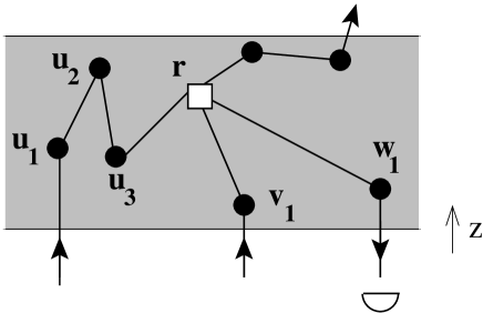
Figure 2: In the perturbative approach, we assume a single nonlinear two-photon scattering event ($\Box$), but arbitrarily many linear scattering events ($\bullet$). One of the two photons is finally annihilated by the detector, thereby defining the photo-detection signal, whereas the other one is scattered into an arbitrary direction.

Now, we generalize the above single-atom treatment to a multiple scattering process in a dilute medium of atoms. First, we note that the above perturbative treatment - in particular Eqs. (19-21) - remains valid for any form of the scattering sample, be it a single atom, two atoms, or arbitrarily many of them. An important difference from the single-atom case, however, is that the total weight of nonlinear processes may be drastically enhanced if the sample has a large optical thickness $b=L/\ell$, where $L$ is the typical medium size. This implies that the condition $s\ll 1$ is not sufficient to guarantee the validity of the perturbative approach. Instead, as we will argue in Sec. IV, the perturbative condition reads $sb^{2}\ll 1$.

A typical two-photon scattering path is sketched in Fig. 2. Here, the incoming photons propagate at first independently from each other to position ${\bf r}$ inside the disordered atomic medium, where they undergo a nonlinear scattering event. One of the two outgoing photons then propagates back to the detector. The possibility that the two photons meet again at another atom can be neglected in the case of a dilute medium, similar to recurrent scattering in the linear case recurr . We can hence restrict our analysis to processes like the one shown in Fig. 2, with arbitrary numbers of linear scattering events before and after the nonlinear one. Thus one of the two incoming photons undergoes $n\geq 0$ elastic scattering events (labeled by ${\bf u_{i}}$), while the other undergoes $m\geq 0$ elastic scattering events (labeled by ${\bf v_{j}}$), before merging at ${\bf r}$ where they undergo the inelastic scattering event. One of the outgoing inelastic photons reaches back the detector after having undergone $l\geq 0$ elastic scattering events (labeled by positions ${\bf w_{k}}$). For the other undetected inelastic photon, we may assume, without any loss of generality, that it does not interact anymore with the atomic medium. This interaction would be anyway described by a unitary operator (as a consequence of energy conservation), which does not change the norm of the state $|\psi\rangle$ of the undetected photon defining the detection signal.

In general, the state of the inelastic undetected photon corresponding to a scattering path $\mathrm{C}$ defined by the position ${\bf r}$ of the two-photon scattering event and by the collection of positions of all one-photon scattering events $\mathrm{C}\equiv\{{\bf u},{\bf v},{\bf r},{\bf w}\}$ is given as follows:

$$|\psi_{\rm in}(\mathrm{C})\rangle=e^{ikn_{\omega}(z_{u_{1}}+z_{v_{1}})}\\ \times\prod_{i=1}^{n}S_{\omega}G_{\omega}({\bf u_{i}},{\bf u_{i+1}})\prod_{j=1}^{m}S_{\omega}G_{\omega}({\bf v_{j}},{\bf v_{j+1}})\\ \times\int d\omega^{\prime}\,\Pi_{\omega^{\prime}}|\psi_{\rm in}\rangle\prod_{k=1}^{l}S_{\omega^{\prime}}G_{\omega^{\prime}}({\bf w_{k}},{\bf w_{k+1}})\\ e^{ikn_{\omega^{\prime}}z_{w_{1}}}\times\begin{cases}1&n=m=0,\\ 2&n>0\text{ or }m>0\end{cases}$$ (27)

with ${\bf u_{n+1}}={\bf v_{m+1}}={\bf w_{l+1}}={\bf r}$, $\Pi_{\omega^{\prime}}$ the projector on photons states at frequency $\omega^{\prime}$ and $|\psi_{\rm in}\rangle$ the inelastic final state of the one-atom case, Eq. (18). Since the inelastic two-photon scattering event takes place at position ${\bf r}$, this state describes an outgoing spherical wave emitted at ${\bf r}$. Furthermore, note that if the two incoming photons do not originate both from the incident mode, i.e. if $n>0$ or $m>0$, a factor $2$ arises due to the fact that the incoming photons can be distributed in two different ways among the paths $\{u\}$ and $\{v\}$.

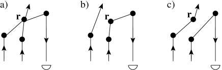
Figure 3: The elastic component $|\psi({\bf r},\{{\bf u},{\bf v},{\bf w}\})_{\rm el}\rangle$ of the undetected photon’s state arises from a superposition of the following three processes: (a) elastic scattering of both photons at ${\bf r}$, (b) only the detected photon scattered at ${\bf r}$, and (c) only the undetected photon scattered at ${\bf r}$. The last two diagrams are necessary to take into account the nonlinear average propagation of the undetected (b) or detected (c) photon.

The elastic component $|\psi_{\rm el}(\mathrm{C})\rangle$ is obtained in a similar way. However, as in the single-atom case, we must take into account forward scattering of the undetected photon, at the position ${\bf r}$ of the nonlinear event. This is done by considering the superposition of two diagrams where the undetected photon is scattered or not scattered at ${\bf r}$, see Fig. 3(a,b). Since this approach exactly parallels the one known from the single-atom case wellens , it is unnecessary to present the complete calculation of the elastic component in detail - all relevant ingredients to perform the generalization to the multi-atom case will be contained in the calculation of the inelastic component. In contrast to the single-atom case, however, the elastic component will enter in the calculation of the nonlinear average propagation, i.e. the nonlinear modification of the refractive index (Kerr effect), and will be discussed later. At first, we concentrate on the processes of nonlinear scattering, i.e. processes changing the direction of propagation of the detected photon.

As for the linear case, we still assume the same dilute medium approximations to hold for the ‘ladder’ and ‘crossed’ contributions. Thus, in order to calculate the average photo-detection signal, we just keep scattering diagrams obtained by reversing the path of the detected photon. Furthermore, we also neglect interference between diagrams where the nonlinear scattering event occurs at different atoms. This is justified in the dilute case since the overlap between two spherical waves emitted at ${\bf r}$ and ${\bf r^{\prime}}$ vanishes if $k|{\bf r}-{\bf r^{\prime}}|\gg 1$.

III.2.3 Nonlinear ladder contribution

To obtain the inelastic component of the average backscattering signal, we first get the total final state of the undetected photon by summing Eq. (27) over all possible different scattering paths $\mathrm{C}$. Then we insert this result into Eq. (21) and we finally average over the random positions of the scatterers. As argued above, only identical or reversed scattering paths are retained in the average, giving rise to the background (‘ladder’) and interference (‘crossed’) component. Thus, the inelastic background component reads as follows:

$$L_{\rm in}^{(2)}=\int_{V}d{\bf r}\sum_{(n,m,l)=0}^{\infty}\frac{{\mathcal{N}}^{n+m+l+1}}{4\pi k^{2}\Sigma}\int_{V}\prod_{i=1}^{n}d{\bf u_{i}}\prod_{j=1}^{m}d{\bf v_{j}}\prod_{k=1}^{l}d{\bf w_{k}}\\ \langle\psi_{\rm in}(\mathrm{C})|\psi_{\rm in}(\mathrm{C})\rangle\times\begin{cases}1&\text{ if }n=m=0\\ 1/2&\text{ otherwise}\end{cases}$$ (28)

Note that some care must be taken not to sum twice over the same scattering path. In particular, any exchange of the two incoming parts $\{u\}$ and $\{v\}$ leaves the total scattering path unchanged since the two incoming photons are identical. For this reason, a factor $1/2$ must be inserted at the end of Eq. (28). Again, as in Eq. (27), the case $n=m=0$ is exceptional, since then there is no elastic scattering events before the nonlinear one: the two incident photons remain in the same mode.

If we insert now Eq. (27) into Eq. (28), we simply obtain the inelastic nonlinear ladder contribution as:

$$L_{\rm in}^{(2)}=s\int\frac{d{\bf r}}{\Sigma\ell}\left(2I^{2}_{\omega}({\bf r})-e^{-2z/\ell}\right)\int d\omega^{\prime}P(\omega^{\prime})I_{\omega^{\prime}}({\bf r}),$$ (29)

with $I_{\omega}({\bf r})$ the linear average intensity, see Eq. (14). In order to interpret this result, we first note that the inelastic intensity radiated by the atom at position ${\bf r}$ is proportional to the mean squared intensity at ${\bf r}$. An alternative, physically transparent derivation of the latter can be performed as follows: we write the local field amplitude $\mathcal{A}=\exp(-z/2\ell)+\mathcal{A}_{D}$ as a sum of coherent and diffuse light amplitudes. The latter term exhibits a Gaussian speckle statistics goodman , i.e. $\langle\mathrm{Re}\mathcal{A}_{D}\rangle=\langle\mathrm{Im}\mathcal{A}_{D}\rangle=0$, $2\langle(\mathrm{Re}\mathcal{A}_{D})^{2}\rangle=2\langle(\mathrm{Im}\mathcal{A}_{D})^{2}\rangle=\langle|\mathcal{A}_{D})|^{2}\rangle$ and $\left<|\mathcal{A}_{D}|^{4}\right>=2\left<|\mathcal{A}_{D}|^{2}\right>^{2}$. Thereby, we obtain for the mean squared intensity:

$$\left<|\mathcal{A}|^{4}\right> = e^{-2z/\ell}+\left<|\mathcal{A}_{D}|^{4}\right>+4e^{-z/\ell}\left<|\mathcal{A}_{D}|^{2}\right>$$ (30)

$$= 2\left<|\mathcal{A}|^{2}\right>^{2}-e^{-2z/\ell}.$$ (31)

Inserting the average intensity, $I_{\omega}=\left<|\mathcal{A}|^{2}\right>$, we immediately recognize the first integrand in Eq. (29). Then, the atom emits a photon with frequency distribution $P(\omega^{\prime})$. Finally, due to time reversal symmetry, the propagation of this photon from ${\bf r}$ to the detector is described by the same function $I_{\omega^{\prime}}({\bf r})$ which represents propagation of incoming photons to ${\bf r}$.

Concerning the elastic component, the diagrammatic calculation via Eq. (20), see also Fig. 3(a,b), shows that the above argument can be repeated in the same way - except for the fact that the detected photon does not change its frequency. Furthermore, a factor $-2$ is taken over from the single-atom expression, cf. Eqs. (23,24). Thereby, we obtain:

$$L_{\rm el}^{(2,{\rm scatt})}=-2s\int\frac{d{\bf r}}{\Sigma\ell}\left(2I^{2}_{\omega}({\bf r})-e^{-2z/\ell}\right)I_{\omega}({\bf r}).$$ (32)

The index ‘scatt’ reminds us that we have treated only nonlinear scattering so far. Below (Sec. III.2.5), we will add nonlinear average propagation, which contributes to the elastic nonlinear component, too.

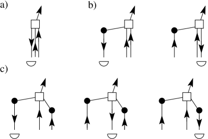
Figure 4: In the presence of nonlinear scattering ($\Box$), there may be either (b) two, or (c) three interfering amplitudes contributing to enhanced backscattering, apart from single scattering (a), which only contributes to the background. In general, the case (c), which corresponds to maximum enhancement factor three, is realized if either both incoming photons, or one incoming and the outgoing detected photon exhibit at least one linear scattering event ($\bullet$) besides the nonlinear one.

III.2.4 Nonlinear crossed contribution

It remains to calculate the ‘crossed’ contribution, i.e. interference between reversed paths. In contrast to the linear case, where there are always two interfering amplitudes (apart from single scattering), the nonlinear case admits more possibilities to reverse the path of the detected photon. This is due to the photon exchange symmetry at the nonlinear scattering event, which does not allow to distinguish which one of the two incoming photons finally corresponds to the detected or undetected one. As evident from Fig. 4(c), each multiple scattering path where both incoming photons, or one incoming and the outgoing detected photon, exhibit at least one linear scattering event besides the nonlinear one, has two different reversed counterparts, leading in total to three interfering amplitudes.

If we look at the scattering process shown in Fig. 2, the two reversed counterparts are obtained by exchanging the outgoing detected photon $\{w\}$ with either one of the incoming photons $\{u\}$ or $\{v\}$. Since both cases are identical in the ensemble average, we may restrict ourselves to one of them, let us say $\{v\}$. We thus note $\widetilde{\mathrm{C}}\equiv\{{\bf u},{\bf w},{\bf r},{\bf v}\}$ the reverse path corresponding to $\mathrm{C}\equiv\{{\bf u},{\bf v},{\bf r},{\bf w}\}$ when $\{v\}$ and $\{w\}$ are exchanged. In total, we obtain for the inelastic interference component:

$$C_{\rm in}^{(2)}=\int_{V}d{\bf r}\sum_{(n,m,l)=0}^{\infty}\frac{{\mathcal{N}}^{n+m+l+1}}{4\pi k^{2}\Sigma}\times\\ \int_{V}\prod_{i=1}^{n}d{\bf u_{i}}\prod_{j=1}^{m}d{\bf v_{j}}\prod_{k=1}^{l}d{\bf w_{k}}\langle\psi_{\rm in}(\mathrm{C})|\psi_{\rm in}(\widetilde{\mathrm{C}})\rangle\\ \times\begin{cases}0&\text{ if }m=l=0\\ 1&\text{ otherwise}\end{cases}$$ (33)

Here, the case $m=l=0$ identifies processes where the two reversed paths $\mathrm{C}$ and $\widetilde{\mathrm{C}}$ are indistinguishable. Setting their contribution equal to zero accounts in particular for the single scattering case depicted in Fig. 4(a), i.e. $n=m=l=0$, which does not contribute to the interference cone. The case Fig. 4(b) remains with two contributions ($n=m=0$, $l>0$, and $n=l=0$, $m>0$, respectively) in Eq. (33), corresponding to the fact that two amplitudes interfere. Finally, the case (c) of three interfering amplitudes is reflected in Eq. (33) by the absence of the exchange factor $1/2$, as compared to the background, Eq. (28). Thereby, the interference contribution can, in principle, become up to two times larger than the background.

If we insert the state of the undetected photon, Eq. (27), into Eq. (33), we encounter the following expression

$$g_{\omega,\omega^{\prime}}({\bf r})=e^{ik(n_{\omega}-n_{\omega^{\prime}}^{*})z}+\sum_{n=1}^{\infty}{\mathcal{N}}^{n}\int_{V}d{\bf r_{1}}\dots d{\bf r_{n}}\\ e^{ik(n_{\omega}-n_{\omega^{\prime}}^{*})z_{1}}\prod_{i=1}^{n}S_{\omega}G_{\omega}({\bf r_{i}},{\bf r_{i+1}})S_{\omega^{\prime}}^{*}G_{\omega^{\prime}}^{*}({\bf r_{i}},{\bf r_{i+1}}),$$ (34)

which generalizes the local intensity, Eq. (13), to the case where two different frequencies occur in the interfering paths. Numerically, it can be obtained as the iterative solution of:

$$g_{\omega,\omega^{\prime}}({\bf r})=e^{ik(n_{\omega}-n_{\omega^{\prime}}^{*})z}+{\mathcal{N}}S_{\omega}S_{\omega^{\prime}}^{*}\\ \times\int_{V}d{\bf r^{\prime}}G_{\omega}({\bf r},{\bf r^{\prime}})G_{\omega^{\prime}}^{*}({\bf r},{\bf r^{\prime}})g_{\omega,\omega^{\prime}}({\bf r^{\prime}}).$$ (35)

This function describes the ensemble-averaged product of two probability amplitudes, one representing an incoming photon with frequency $\omega$ propagating to position ${\bf r}$, and the other one the complex conjugate of a photon with frequency $\omega^{\prime}$ propagating from ${\bf r}$ to the detector. If $\omega\neq\omega^{\prime}$, then these amplitudes display a nonvanishing phase difference both due to scattering and to average propagation in the medium. This leads on average to a decoherence mechanism and consequently to a loss of interference contrast. Indeed, both the complex scattering amplitude, Eq. (1), and the refractive index, Eq. (5), depend on frequency. In contrast, the phase difference due to free propagation (i.e. in the vacuum) can be neglected if $\Gamma\ell\ll c$, which is fulfilled for typical experimental parameters thierry ; havey2 . In the case $\omega=\omega^{\prime}$ of identical frequencies, $g_{\omega,\omega}({\bf r})=I_{\omega}({\bf r})$ reduces to the average intensity, see Eq. (14).

In terms of the iterative solution of Eq. (34), the inelastic interference term, Eq. (33), is rewritten as follows:

$$C_{\rm in}^{(2)}= 4s\int d\omega^{\prime}P(\omega^{\prime})\int_{V}\frac{d{\bf r}}{\Sigma\ell}\Bigl{[}I_{\omega}({\bf r})|g_{\omega,\omega^{\prime}}({\bf r})|^{2}\Bigr{.}$$ (36)

$$-e^{-z/\ell}{\rm Re}\left\{e^{i(n_{\omega}-n_{\omega^{\prime}}^{*})kz}g_{\omega,\omega^{\prime}}^{*}({\bf r})\right\}$$

$$\Bigl{.}-\left(I_{\omega}({\bf r})-e^{-z/\ell}\right)e^{-z/\ell-z/\ell^{\prime}}\Bigr{]},$$

with $\ell^{\prime}$ the linear mean free path at frequency $\omega^{\prime}$. In the elastic case, where $\omega^{\prime}=\omega$, dephasing between reversed scattering paths does not occur, and the expression (36) simplifies to:

$$C_{\rm el}^{(2,{\rm scatt})}=-8s\int_{V}\frac{d{\bf r}}{\Sigma\ell}\left(I_{\omega}({\bf r})^{3}-2I_{\omega}({\bf r})e^{-2z/\ell}+e^{-3z/\ell}\right).$$ (37)

Since, in the elastic case, there is no loss of coherence due to change of frequency, the elastic interference component, Eq. (37), is completely determined by the relative weights of the one-, two-, and three-amplitudes cases exemplified in Fig. 4. This can be checked by rewriting the background and interference components, Eqs. (32,37), in terms of diffuse and coherent light, respectively, i.e. by writing $I=I_{D}+\exp(-z/\ell)$. One obtains:

$$L_{\rm el}^{(2,{\rm scatt})} \propto\bigl{<}e^{-3z/\ell}+5I_{D}e^{-2z/\ell}+~{}6I_{D}^{2}e^{-z/\ell}+2I_{D}^{3}\bigr{>},$$ (38)

$$C_{\rm el}^{(2,{\rm scatt})} \propto\bigl{<}\underbrace{\phantom{e^{-3z/\ell}+\!}}_{\displaystyle(a)}~{}\underbrace{4I_{D}e^{-2z/\ell}}_{\displaystyle(b)}+\underbrace{12I_{D}^{2}e^{-z/\ell}+4I_{D}^{3}}_{\displaystyle(c)}\bigr{>},$$

where the brackets denote the integral over the volume $V$ of the medium, and (a,b,c) correspond to the three cases shown in Fig. 4, identified by different powers of diffuse or coherent light. As expected, the three-amplitudes case (c) implies an interference term twice as large as the background. In the two-amplitudes case (b), a small complication arises, since one of the two interfering amplitudes is twice as large as the other one (i.e. the one where both incoming photons originate from the coherent mode), cf. the discussion after Eq. (27). In this case, the interference contribution, $2\times 1+1\times 2=4$, is smaller than the background, $2\times 2+1\times 1=5$. Finally, as it should be, the single scattering term (a) is absent in the interference term $C_{\rm el}^{(2,{\rm scatt})}$.

III.2.5 Nonlinear average propagation

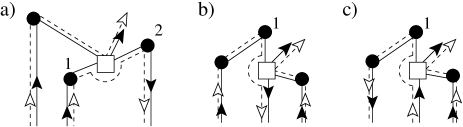
Figure 5: Diagrammatic description of nonlinear propagation. A two-photon process (solid lines) interferes with two independent single photons (dashed lines). Only one of the latter (the undetected photon) is scattered at $\Box$, thereby modifying the propagation of the detected photon (a) between two scattering events at positions 1 and 2, (b) on the way to the detector after the last scattering event at position 1, or (c) in the coherent mode before the first scattering event at position 1.

So far, we have only considered processes of nonlinear scattering where the direction of propagation of the detected photon is changed. It remains to take into account nonlinear average propagation. This is described by those processes where, in one of the two interfering amplitudes, the detected photon is not scattered at the position ${\bf r}$ of the nonlinear event . The corresponding diagrams are depicted in Fig. 5, where the two interfering amplitudes are represented by the solid and dashed lines, respectively. Here, the solid lines correspond to an inelastic two-photon scattering process (like the one shown in Fig. 2), whereas the dashed lines represent an elastic process, where the two photons are independent from each other, see Fig. 3(c). Hence, their interference contributes to the nonlinear elastic component of the photo-detection signal, cf. Eq. (20).

The three diagrams shown in Fig. 5 differ only by the fact that the nonlinear propagation event takes place either between two scattering events at position 1 and 2 (a), on the way to the detector, i.e. after the last scattering event at position 1 (b), or in the coherent mode, i.e. before the first scattering event at position 1 (c). At first, let us examine the case (a). We imagine that each of the three dots $\bullet$ may represent an arbitrary number of scattering events. [Only note that the number of events corresponding to the dots and 1 and 2 must be larger than zero - otherwise, the diagram Fig. 5(a) would be identical to Fig. 5(b) or (c).] According to the theory of linear radiative transfer outlined in Sec. III.1, the ladder diagrams corresponding to the two incoming photons arriving at 1 (position ${\bf r_{1}}$) and at the nonlinear event $\Box$ (position ${\bf r_{3}}$) yield the linear local intensities $I_{\omega}({\bf r_{1}})$ and $I_{\omega}({\bf r_{3}})$, respectively. Likewise (due to reciprocity symmetry), the propagation of the outgoing detected photon from 2 (position ${\bf r_{2}}$) to the detector - with arbitrary number of scattering events in between - is given by $I_{\omega}({\bf r_{2}})$. Hence, the only ingredient which we have to calculate is the nonlinear propagation between 1 and 2. Note that, when taking the average over the position ${\bf r_{3}}$ of the nonlinear event, non-negligible contributions arise only if ${\bf r_{3}}$ is situated on the straight line between ${\bf r_{1}}$ and ${\bf r_{2}}$, since this is the only way to fulfill a stationary phase (or phase matching) condition. Thereby, the ‘pump intensity’ entering in the nonlinear propagation is given by the average value of the local intensity on this line, which we denote by $\langle I_{\omega}\rangle_{{\bf r_{1}}\to{\bf r_{2}}}$. We do not want to present the complete calculation here (this requires to calculate at first the case of a single atom, which can be done with the techniques described in wellens ), but just give the final result:

$$\left|G_{\omega}^{(\rm nl,a)}({\bf r_{1}},{\bf r_{2}})\right|^{2}=\left|G_{\omega}({\bf r_{1}},{\bf r_{2}})\right|^{2}\frac{2sr_{12}}{\ell}\langle I_{\omega}\rangle_{{\bf r_{1}}\to{\bf r_{2}}}.$$ (39)

From this, we deduce the following value for the nonlinear mean free path:

$$\frac{1}{\ell^{(\rm nl)}({\bf r})}=\frac{1}{\ell}\left(1-2sI_{\omega}({\bf r})\right),$$ (40)

which is consistent with Eq. (39), if we expand the resulting propagator (where the mean free path appears in the exponent) up to first order in $s$. The same result is also obtained in the case of diagram Fig. 5(b), i.e. for the propagation after the last scattering event. Hence, the corresponding propagator (first order in $s$) reads:

$$\left|G_{\omega}^{(\rm nl,b)}({\bf r_{1}})\right|^{2}=e^{-z_{1}/\ell}\frac{2sz_{1}}{\ell}\langle I_{\omega}\rangle_{{\bf r_{1}}\to{\bf r_{0}}},$$ (41)

where ${\bf r_{0}}={\bf r_{1}}-z_{1}{\bf e_{z}}$, with ${\bf e_{z}}$ the unit vector pointing in the direction of the incident laser, denotes the point where the photon leaves the medium. In the case (c), a small complication arises since the photons arriving at the nonlinear event $\Box$ may originate both from the coherent mode, which reduces the two-photon scattering amplitude by a factor $1/2$, cf. the discussion after Eq. (27). Hence, the nonlinear mean free path for photons from the coherent mode reads:

$$\frac{1}{\ell_{c}^{(\rm nl)}({\bf r})}=\frac{1}{\ell}\left(1-2sI_{\omega}({\bf r})+se^{-z/\ell}\right),$$ (42)

with the corresponding propagator

$$\left|G_{\omega}^{(\rm nl,c)}({\bf r_{1}})\right|^{2}=e^{-z_{1}/\ell}\frac{sz_{1}}{\ell}\left<2I_{\omega}({\bf r})-e^{-z/\ell}\right>_{{\bf r_{0}}\to{\bf r_{1}}},$$ (43)

The difference between the mean free paths, Eqs. (40,42), can also be understood as a consequence of the different properties of intensity fluctuations for diffuse and coherent light, see Eq. (30), which determine the nonlinear atomic response.

In total, we obtain for the background component:

$$L_{\rm el}^{(2,{\rm prop})}=\frac{\mathcal{N}}{\Sigma\ell}\int_{V}d{\bf r_{1}}d{\bf r_{2}}I_{\omega}({\bf r_{1}})I_{\omega}({\bf r_{2}})\left|S_{\omega}G_{\omega}^{(\rm nl,a)}({\bf r_{1}},{\bf r_{2}})\right|^{2}\\ +\int_{V}\frac{d{\bf r_{1}}}{\Sigma\ell}I_{\omega}({\bf r_{1}})\left(\left|G_{\omega}^{(\rm nl,b)}({\bf r_{1}})\right|^{2}+\left|G_{\omega}^{(\rm nl,c)}({\bf r_{1}})\right|^{2}\right).$$ (44)

In the case of a slab of length $L$, Eq. (44) can be simplified to:

$$L_{\rm el}^{(2,{\rm prop})}=s\int_{0}^{L}\frac{dz}{\ell}I_{\omega}(z)\left(2I_{\omega}(z)^{2}-2I_{\omega}^{2}(L)\right.\\ \bigl{.}+e^{-2z/\ell}-e^{-z/\ell}\bigr{)}.$$ (45)

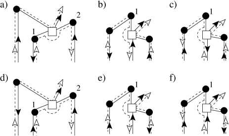
Figure 6: Interference contributions from nonlinear propagation. The diagrams (a-f) are obtained from the ladder diagrams, see Fig. 5, by reversing the paths of the respective photons. Just as in the case of nonlinear scattering, there are twice as many diagrams contributing to the interference cone than to the background.

Concerning the interference component, we find the same phenomenon which we have already observed in the case of nonlinear scattering: if we exchange outgoing and incoming propagators, we find twice as many ‘crossed’ as ‘ladder’ diagrams, see Fig. 6. In particular, the diagrams (d,e,f), which could be seen as a modification of the linear refractive index by the local crossed intensity - thus affecting the (ladder) average propagation - are not considered in previously published papers, concerning either classical linear scatterers in a non-linear medium cbsnl1 ; cbsnl2 or nonlinear scatterers in the vacuum wellens2 ; erratum . Even if, at first sight, these diagrams look unusual, our numerical calculations (see section III.4) suggest that they play an important role, at least in our situation where nonlinear scattering and nonlinear propagation originate from the same microscopic process.

Due to the reciprocity symmetry (remember that nonlinear propagation contributes to the elastic component, i.e. no decoherence due to change of frequency ), each of the diagrams in Fig. 6 gives the same contribution as the corresponding ladder diagram in Fig. 5. Hence, to first approximation, the interference contribution from nonlinear propagation equals twice the background, Eq. (44). Some care must be taken, however, if photons arriving at (or departing from) the nonlinear event (or position 1) originate from the coherent mode. In such cases, it may happen that some of the diagrams depicted in Figs. 5 and 6 coincide, and we should not count them twice. [This is analogous to the distinction between the cases (a,b,c) in Fig. 4, or to the suppression of single scattering in the linear case.]

Taking this into account [for details, we refer to the discussion after Eq. (71) in appendix A], we find:

$$C_{\rm el}^{(2,{\rm prop})}=2L_{\rm el}^{(2,{\rm prop})}-3\int_{V}\frac{d{\bf r_{1}}}{\Sigma\ell}\left[e^{-z_{1}/\ell}\left|G_{\omega}^{(\rm nl,c)}({\bf r_{1}})\right|^{2}\right.\\ \left.+I({\bf r_{1}})e^{-z_{1}/\ell}s\left(1-e^{-z_{1}/\ell}\right)\right].$$ (46)

In the case of a slab, we obtain:

$$C_{\rm el}^{\rm(2,prop)}=2L_{\rm el}^{(2,{\rm prop})}-3s\int_{0}^{L}\frac{dz}{\ell}I(z)\left[e^{-z/\ell}-e^{-2b}\right]\\ +s\left(\frac{1}{2}-\frac{3}{2}e^{-2b}+e^{-3b}\right),$$ (47)

where $b=L/\ell$ denotes the (linear) optical thickness of the slab.

Thereby, we have completed the perturbative calculation of the backscattering signal for the scalar case. The total signal is obtained as the sum of the various components discussed above:

$$L = L_{\rm el}^{(1)}+L_{\rm el}^{(2,{\rm scatt})}+L_{\rm el}^{(2,{\rm prop})}+L_{\rm in}^{(2)},$$ (48)

$$C = C_{\rm el}^{(1)}+C_{\rm el}^{(2,{\rm scatt})}+C_{\rm el}^{(2,{\rm prop})}+C_{\rm in}^{(2)}.$$ (49)

Before we present the numerical results in Sec. IV, we will generalize the above results to the vectorial case. This is important since polarization does not only lead to slight modifications for low scattering orders, as in the linear case. Apart from that, we will see that it also induces decoherence between reversed paths, thereby reducing the nonlinear interference components.

III.3 Incorporation of polarization : vectorial case

First, including the polarization modifies the scalar expressions, Eqs. (1,6), for the linear mean free path and the atom-photon scattering amplitude by a factor $2/3$:

$$\hat{\ell} = \left(1+\frac{4\delta^{2}}{\Gamma^{2}}\right)\frac{k^{2}}{6\pi{\mathcal{N}}},$$ (50)

$$\tilde{S}_{\omega} = \frac{-6\pi i}{k(1-2i\delta/\Gamma)}$$ (51)

The Green’s function, Eq. (4), remains unchanged, except for the fact that the modified expression for the mean free path, Eq. (50), must be inserted in the refractive index. However, the angular anisotropic character of the atom-photon scattering is not yet contained in Eq. (51). This is treated by projection of the polarization vector as follows: if the photon, with incoming polarization $\epsilon_{1}$, is scattered at ${\bf r_{1}}$, and the next scattering event takes place at ${\bf r_{2}}$, the new incoming polarization reads:

$$\epsilon_{2}=\Delta_{{\bf r_{1}},{\bf r_{2}}}\epsilon_{1},$$ (52)

where $\Delta_{{\bf r_{1}},{\bf r_{2}}}$ denotes the projection onto the plane perpendicular to ${\bf r_{1}}-{\bf r_{2}}$. Finally, the detection signal after $n$ scattering events is obtained as $\epsilon_{D}^{*}\cdot\epsilon_{n}$, with the detector polarization $\epsilon_{D}$.

Thus, the linear background (‘ladder’) contribution reads, cf. Eqs. (8,11):

$$\hat{L}^{(1,\rm el)}=\sum_{n=1}^{\infty}\int\frac{d{\bf r_{1}}}{A\hat{\ell}}{\mathcal{N}}^{n-1}\int_{V}d{\bf r}_{2}\dots d{\bf r}_{n}~{}e^{-z_{1}/\hat{\ell}}\\ \times\left(\prod_{i=1}^{n-1}|\hat{S}_{\omega}\hat{G}_{\omega}({\bf r_{i}},{\bf r_{i+1}})|^{2}\right)e^{-z_{n}/\hat{\ell}}\\ \times\frac{3}{2}\left|\epsilon_{D}^{*}\Delta_{{\bf r_{n-1}},{\bf r_{n}}}\dots\Delta_{{\bf r_{1}},{\bf r_{2}}}\epsilon_{L}\right|^{2},$$ (53)

where $\epsilon_{L}$ denotes the initial laser polarization. By choosing a given circular polarization, for example $\epsilon_{L}=(1,i,0)/\sqrt{2}$, and by detecting the signal in the helicity-preserving $h\parallel h$ polarization channel ($\epsilon_{D}=\epsilon_{L}^{*}$), then the single scattering contribution in Eq. (53) ($n=1$ term) is filtered out. We thus recover the enhancement factor $2$, meaning $C_{\rm el}^{(1)}=L_{\rm el}^{(1)}$. Apart from that, however, polarization does not play a very important role: the distribution of higher scattering orders $n>1$ is only slightly modified, and the reciprocity symmetry remains valid, provided that $\epsilon_{D}=\epsilon_{L}^{*}$.

Figure 7: Polarization vectors associated to the two-photon scattering matrix for two reversed scattering amplitudes (a) and (b). Note that the corresponding reversed scattering amplitudes, Eqs. (54,56) are different - even in the helicity preserving polarization channel, i.e. if $\tilde{\epsilon}_{2,3}=\epsilon_{2,3}^{*}$. This leads to a reduction of the CBS interference cone by a factor 3/4, on average.

The situation changes in the nonlinear regime of two-photon scattering. With the initial and final polarizations $\epsilon_{1,2}$ and $\epsilon_{3,4}$, respectively, see Fig. 7(a), the polarization dependent term of the two-photon scattering matrix reads:

$$S_{p}=\frac{1}{2}\left[(\epsilon_{1}\cdot\epsilon_{4}^{*})(\epsilon_{2}\cdot\epsilon_{3}^{*})+(\epsilon_{1}\cdot\epsilon_{3}^{*})(\epsilon_{2}\cdot\epsilon_{4}^{*})\right].$$ (54)

The prefactor $1/2$ is chosen such that $S_{p}$ represents correctly the polarized scattering amplitude in units of the corresponding scalar one. From Eq. (54), the photon exchange symmetry becomes evident: the outgoing photon 3, e.g., can equally well be associated with the incoming photon 1 or 2. If we trace over the undetected photon, which we may label as photon 4, for example, we obtain for the ladder component:

$$\Pi^{(L)}(\epsilon_{1},\epsilon_{2};\epsilon_{3})=\sum_{\epsilon_{4}}|S_{p}|^{2}=\frac{1}{4}\Bigl{[}|\epsilon_{2}\cdot\epsilon_{3}^{*}|^{2}+|\epsilon_{1}\cdot\epsilon_{3}^{*}|^{2}\Bigr{.}\\ \left.+2{\rm Re}\Bigl{\{}(\epsilon_{1}\cdot\epsilon_{2}^{*})(\epsilon_{2}\cdot\epsilon_{3}^{*})(\epsilon_{3}\cdot\epsilon_{1}^{*})\Bigr{\}}\right].$$ (55)

If we assume a random uniform distribution for the polarization vectors, we obtain $\langle\Pi^{(L)}\rangle=2/9$, which is smaller than the linear counterpart $\langle|\epsilon_{n}\cdot\epsilon_{D}^{*}|^{2}\rangle=1/3$. Hence, in the vectorial case, the relative weight of the nonlinear contribution is approximately one third smaller than in the scalar case - at least far inside the medium, where the polarization is sufficiently randomized.

Concerning the interference (‘crossed’) contribution, we exchange the direction of the outgoing detected photon 3 and of one of the incoming photons, for example photon 2. Note that we obtain in general different polarizations $\tilde{\epsilon}_{2,3}$ for the reversed counterparts of $\epsilon_{2,3}$, see Fig. 7(b). Indeed, the reversed photons have the same polarizations, $\tilde{\epsilon}_{2,3}=\epsilon_{2,3}$, only if the laser and detector polarizations are identical ($\epsilon_{D}=\epsilon_{L}$). Consequently, the scattering amplitude for the complex conjugate photon pair reads:

$$\tilde{S}_{p}=\frac{1}{2}\left[(\epsilon_{1}\cdot\epsilon_{4}^{*})(\tilde{\epsilon}_{3}\cdot\tilde{\epsilon}_{2}^{*})+(\epsilon_{1}\cdot\tilde{\epsilon}_{2}^{*})(\tilde{\epsilon}_{3}\cdot\epsilon_{4}^{*})\right].$$ (56)

Note that even in the helicity-preserving polarization channel, i.e. $\tilde{\epsilon}_{2,3}=\epsilon_{2,3}^{*}$, the reversed scattering amplitudes, Eqs. (54,56), are in general not equal. Only the first term, where photon 2 is associated with photon 3, remains unchanged if those two photons are reversed. As a consequence, the polarization induces a loss of coherence, i.e. a reduction of the crossed term as compared to the scalar case. The sum over the polarization of photon 4 yields:

$$\Pi^{(C)}(\epsilon_{1},\epsilon_{2},\tilde{\epsilon}_{3},\epsilon_{3},\tilde{\epsilon}_{2})=\sum_{\epsilon_{4}}S_{p}\tilde{S}_{p}^{*}=\\ =\frac{1}{4}\left[(\epsilon_{2}\cdot\epsilon_{3}^{*})(\tilde{\epsilon}_{2}\cdot\tilde{\epsilon}_{3}^{*})+(\epsilon_{2}\cdot\epsilon_{3}^{*})(\epsilon_{1}\cdot\tilde{\epsilon}_{3}^{*})(\tilde{\epsilon_{2}}\cdot\epsilon_{1}^{*})\right.\\ \left.+(\epsilon_{1}\cdot\epsilon_{3}^{*})(\epsilon_{2}\cdot\tilde{\epsilon}_{3}^{*})(\tilde{\epsilon_{2}}\cdot\epsilon_{1}^{*})+(\epsilon_{1}\cdot\epsilon_{3}^{*})(\epsilon_{2}\cdot\epsilon_{1}^{*})(\tilde{\epsilon_{2}}\cdot\tilde{\epsilon_{3}}^{*})\right].$$ (57)

If we assume $\tilde{\epsilon}_{2,3}=\epsilon^{*}_{2,3}$, i.e. the $h\parallel h$ channel, we obtain $\langle\Pi^{(C)}\rangle=3/18$ on average. Hence, in this channel, the polarization-induced loss of contrast is approximately $\langle\Pi^{(C)}\rangle/\langle\Pi^{(L)}\rangle=3/4$.

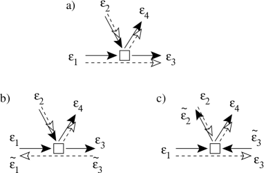
Figure 8: Polarization dependence of nonlinear propagation for (a) ladder and (b,c) crossed diagrams.

Finally, to obtain the polarization dependence of nonlinear propagation, we label the photons as shown in Fig. 8. Let us first examine the ladder term, Fig. 8(a). The solid lines are described by the two-photon amplitude, Eq. (54), whereas the dashed lines give the complex conjugate of $(\epsilon_{2}\cdot\epsilon_{4}^{*})(\epsilon_{1}\cdot\epsilon_{3}^{*})$. After integration over photon 4, the result is

$$\Pi^{(L,\text{prop})}(\epsilon_{1},\epsilon_{2},\epsilon_{3})= \frac{1}{2}\left[(\epsilon_{1}\cdot\epsilon_{2}^{*})(\epsilon_{2}\cdot\epsilon_{3}^{*})(\epsilon_{3}\cdot\epsilon_{1}^{*})\right.$$ (58)

$$+\left.(\epsilon_{1}\cdot\epsilon_{3}^{*})(\epsilon_{2}\cdot\epsilon_{2}^{*})(\epsilon_{3}\cdot\epsilon_{1}^{*})\right].$$

Concerning the crossed diagrams, we distinguish between the two cases shown in Fig. 8(b) and (c). [In Fig. 6, this corresponds to (a,b,c), on the one hand, and (d,e,f), on the other hand.] As for the case (b), nothing changes since the reversed photon does not participate in the nonlinear event. In case (c), we obtain:

$$\Pi^{(C,\text{prop})}(\epsilon_{1},\epsilon_{2},\epsilon_{3},\tilde{\epsilon}_{2},\tilde{\epsilon}_{3})=\frac{1}{2}\left[(\epsilon_{1}\cdot\epsilon_{2}^{*})(\tilde{\epsilon_{3}}\cdot\tilde{\epsilon_{2}}^{*})(\epsilon_{3}\cdot\epsilon_{1}^{*})\right.\\ +\left.(\epsilon_{1}\cdot\tilde{\epsilon_{2}}^{*})(\tilde{\epsilon_{3}}\cdot\epsilon_{2}^{*})(\epsilon_{3}\cdot\epsilon_{1}^{*})\right].$$ (59)

When determining the average values of the nonlinear propagation terms, it must be taken into account that $\epsilon_{1}$ and $\epsilon_{3}$ are not independent from each other, since they propagate in the same (or opposite) direction. Thus, we find $\langle\Pi^{(L,\text{prop})}\rangle=1/3$ and $\langle\Pi^{(C,\text{prop})}\rangle=1/6$. Hence, the loss of contrast equals $1/2$ in case (c), whereas reciprocity remains conserved (i.e. no loss of contrast) in case (b). Averaging over (b) and (c), this yields the same contrast $3/4$ as for nonlinear scattering.

What remains to be done to obtain the vectorial backscattering signal is to incorporate the above expressions into the corresponding scalar equations. The resulting equations can be found in appendix A, together with a description of the Monte-Carlo method which we use for their numerical solution.

III.4 Classical model

We want to stress that our perturbative theory of nonlinear coherent backscattering is not only valid for an atomic medium, but can be adapted to other kinds of nonlinear scatterers. In particular, the effect of interference between three amplitudes is always present in the perturbative regime of a small $\chi^{(3)}$ nonlinearity. Specifically, we have also examined the following model: a collection of classical isotropic scatterers, situated at positions ${\bf r_{i}}$, $i=1,\dots,N$. In analogy to the atomic model, we assume that the field scattered elastically by an individual scatterer at position ${\bf r_{i}}$ is proportional to $E_{i}/(1+s|E_{i}|^{2})$, where $E_{i}$ is the local field at ${\bf r_{i}}$, and $s$ measures the strength of the nonlinearity. Writing $E_{i}$ as a sum of the incident field, and the field radiated by all other scatterers, we obtain the following set of nonlinear equations:

$$E_{i}=e^{i{\bf k_{L}}\cdot{\bf r_{i}}}+i\sum_{j\neq i}\frac{e^{ikr_{ij}}}{kr_{ij}}\frac{E_{j}}{1+s|E_{j}|^{2}}.$$ (60)

Employing diagrammatic theory similar to the one outlined above, we have checked that, in the ensemble average over the positions ${\bf r_{i}}$, this model indeed reproduces the elastic components of the backscattering signal of the atomic model. We have checked that the results obtained from direct numerical solutions of the field equations (60) - averaged over a sufficiently large sample of single realizations - agree with our theoretical predictions, in the perturbative regime of small nonlinearity $s$. In particular, the diagrams (d,e,f) of Fig. 6, describing the interference contributions from the nonlinear propagation, are essential to give the correct results. A more detailed analysis will be presented elsewhere.

Furthermore, it remains to be clarified whether the diagrams (d,e,f) are also relevant for the description of propagation in homogeneous nonlinear media, into which linear scatterers are embedded at random positions. First studies of the resulting CBS cone have been presented in cbsnl1 ; cbsnl2 , without taking into account interference between three amplitudes, however. Experimentally, this question can be resolved by measuring the value of the backscattering enhancement factor $\eta$: whereas $\eta$ is basically unaffected by the nonlinearity according to cbsnl1 ; cbsnl2 (i.e. $\eta=2$ apart from single scattering), our equations (44,46), with $s$ proportional to the incoming intensity and to the $\chi^{(3)}$ coefficient of the nonlinear Kerr medium, predict a significant change of $\eta$ when varying the incoming intensity.

IV Results

We return to the atomic model, concentrating on the case of a slab geometry in the following. Using the equations derived in Sec.  III.1-III.3, we are able to calculate the backscattered intensity up to first order in the saturation parameter $s$. In this section, we will examine its dependence on the optical thickness $b$ and detuning $\delta$, for the scalar and vectorial case. The main quantity of interest is the backscattering enhancement factor $\eta$. It is defined as the ratio between the total detection signal in exact backscattering direction divided by the background component. If we perform an expansion up to first order in $s$, we obtain

$$\eta=\frac{L+C}{L}\simeq\eta^{(1)}+(\eta^{(1)}-1)(\gamma_{C}-\gamma_{L})s.$$ (61)

Here, $\eta^{(1)}=1+C_{\rm el}^{(1)}/L_{\rm el}^{(1)}$ is the enhancement factor in the linear case (i.e. the limit of vanishing saturation). If single scattering is excluded (e.g. in the $h\parallel h$ channel), we have $\eta^{(1)}=2$. Increasing saturation changes the enhancement factor, and the present approach allows us to calculate the slope $d\eta/ds$ of this change at $s=0$. It is given by the difference between the nonlinear crossed and ladder contribution, normalized as follows:

$$\gamma_{L} = \frac{L-L^{(1)}}{sL^{(1)}},$$ (62)

$$\gamma_{C} = \frac{C-C^{(1)}}{sC^{(1)}}.$$ (63)

Obviously, an important question is the domain of validity of the linear expansion, Eq. (61). Strictly speaking, this question can only be answered if we know higher orders of $s$. However, a rough quantitative estimation can be given as follows: if $p_{1}$ (resp. $p_{2+}$) denotes the probability for a backscattered photon to undergo one (resp. more than one) nonlinear scattering event, the perturbative condition reads $p_{2+}\ll p_{1}$. If we assume that all scattering events have the same probability (proportional to $s$) to be nonlinear (thereby neglecting the inhomogeneity of the local intensity), we obtain $p_{1}\simeq\langle N\rangle s$, and $p_{2+}\simeq\langle N^{2}\rangle s^{2}$, where $N$ denotes the total number of scattering events, and $\langle\dots\rangle$ the statistical average over all backscattering paths. Evidently, $N$ and $N^{2}$ are expected to increase when increasing the optical thickness $b$. For a slab geometry, we have found numerically that $\langle N\rangle\propto b$ and $\langle N^{2}\rangle\propto b^{3}$ (in the limit of large $b$), concluding that the perturbative treatment is valid if $sb^{2}\ll 1$. Let us note that a similar condition also ensures the stability of speckle fluctuations in a nonlinear medium skipetrov .

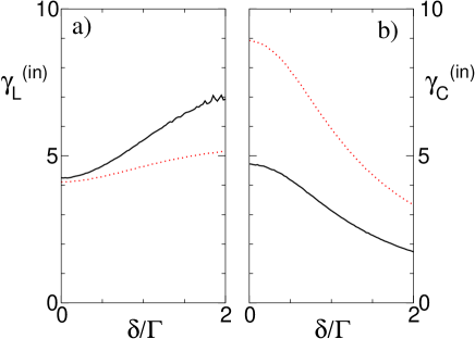
Figure 9: (color online). Normalized inelastic ladder and crossed contributions $\gamma_{L,C}^{(\rm in)}$, cf. Eqs. (62,63), for optical thickness $b=0.5$, as a function of the laser detuning $\delta$. Solid lines: polarized case ($h||h$ channel). Dotted lines: scalar case. For comparison, the corresponding elastic contributions (independent of $\delta$) are $\gamma_{L}^{(\rm el)}=-7.04$ ($h\parallel h$), $-6.53$ (scalar), and $\gamma_{C}^{(\rm el)}=-9.56$ ($h\parallel h$), $-18.8$ (scalar).

In Fig. 9, we show the inelastic ladder and crossed contributions $\gamma_{L}^{(\rm in)}$ and $\gamma_{C}^{(\rm in)}$ for a slab of optical thickness $b=0.5$ as a function of the detuning, $\delta=\omega-\omega_{\rm at}$, for the polarized ($h\parallel h$) and scalar case. Since the optical thickness is kept constant, the elastic quantities are independent of the detuning, and only the inelastic components are affected by $\delta$, via the shape of the power spectrum $P(\omega^{\prime})$ of the inelastically scattered light, see Eq. (26). The latter exhibits two peaks of width $\Gamma$, one of which is centered around the atomic resonance. The increase of the ladder term as a function of $\delta$, which is observed in Fig. 9(a) is due to initially detuned photons, i.e. $\omega=\omega_{\rm at}+\delta$, which are set to resonance ($\omega^{\prime}\simeq\omega_{\rm at}$) by the nonlinear scattering process. For these photons, the scattering cross section increases, which increases the contribution to the backscattering signal in the sum over all scattering orders - especially in the $h\parallel h$ case where single scattering is filtered out. The same effect also applies for the crossed term, Fig. 9(b), but here the dephasing between the reversed paths due to the frequency change - which is more effective for higher values of the detuning - is dominant, leading in total to a decrease of $\gamma_{C}^{(\rm in)}$ as a function of $\delta$. The small ripples in Fig. 9(a), for the polarized case (solid line) at large $\delta$, are due to numerical noise in the Monte-Carlo integration.

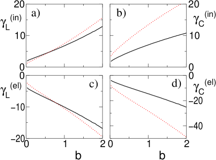
Figure 10: (color online). Normalized inelastic and elastic ladder and crossed $\gamma_{L,C}^{(\rm el,in)}$, cf. Eqs. (62,63), for vanishing detuning $\delta=0$, as a function of the optical thickness $b=0.5$. Solid lines: polarized case ($h||h$ channel). Dotted lines: scalar case.

Fig. 10 shows the elastic and inelastic ladder and crossed contributions, as a function of the optical thickness, at detuning $\delta=0$. The main purpose of this figure is to show the increase of the nonlinear contributions as a function of $b$, which is important to understand the domain of validity of the present approach. The origin of this increase is simple to understand: for larger values of the optical thickness, the average number of scattering events increases, and so does also the probability that at least one of them is a nonlinear one. Thus, for an optically thick medium, even a very small initial saturation may lead to a large inelastic component of the backscattered light. Note, however, that the elastic and inelastic ladder contributions, Fig. 10(a,c), tend to cancel each other, such that their sum depends less strongly on $b$. Physically, this fact is related to energy conservation. The latter ensures that the total nonlinear scattered intensity - integrated over all final directions - vanishes even exactly, since the total outgoing intensity must equal the incident intensity (meaning a purely linear relationship between outgoing and incident intensity).

Furthermore, we note that both the elastic and inelastic ladder components increase significantly slower in the polarized than in the scalar case (solid vs. dashed line). This is due to the fact that, as discussed in Sec. III.3, polarization effects diminish the weight of nonlinear scattering by approximately 2/3. Concerning the crossed components, Fig. 10(b,d), the difference is even stronger, due to the additional polarization-induced loss of contrast by a factor $3/4$, in average. Please note that the vertical scale for the elastic crossed case, Fig. 10(d), is two times larger than in the other three cases: this reflects the effect of interference between three amplitudes, which renders the crossed component up to two times larger than the ladder. Concerning the inelastic component, Fig. 10(b), this effect is diminished by decoherence due to the frequency change at inelastic scattering. Here, crossed and ladder component are of similar magnitude.

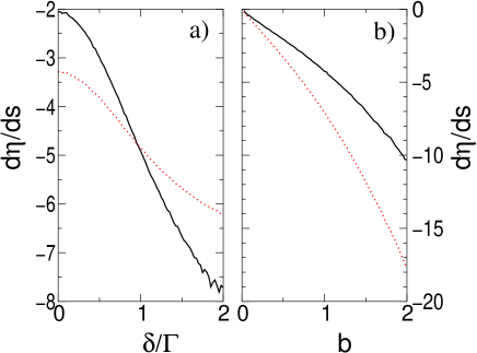
Figure 11: (color online). Slope of backscattering enhancement factor, for the parameters of Fig. 9 ($b=0.5$, left half) and Fig. 10 ($\delta=0$, right half). Solid lines: polarized case ($h||h$ channel). Dotted lines: scalar case.

In Fig. 11, we show the slope of the backscattering enhancement factor, which follows via Eq. (61) from the data shown in Figs. 9 and 10. Fig. 11(b) again points out the importance of even small saturation in the case of an optically thick medium. For example, in the scalar case at $b=2$, increasing the saturation from $s=0$ to $s=0.01$ decreases the enhancement factor from $1.73$ ($<2$ due to single scattering) to $1.55$. For very large $b$, we find a linear decrease of the slope. At the same time, however, the allowed domain of $s\ll 1/b^{2}$ shrinks to zero quadratically. This allows the enhancement factor to remain a continuous function of $s$, even in the limit $b\to\infty$, where its slope at $s=0$ diverges. In order to make more precise statements about the behavior in the limit $b\to\infty$, however, it is necessary to generalize our theory to the case of more than one nonlinear scattering event.

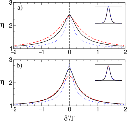
Figure 12: (color online). Spectral dependence of the enhancement factor, for detuning $\delta=0$ and optical thickness $b=0.5$ (dashed line), $1$ (solid), and $2$ (dotted), in the $h\parallel h$ channel (a) and the scalar case (b). The vertical dashed line displays the position of the elastic $\delta$ peak, which must be filtered out in order to observe an enhancement factor larger than two. The inset shows the power spectrum of the backscattered light (background component), which is almost identical with the single-atom spectrum.

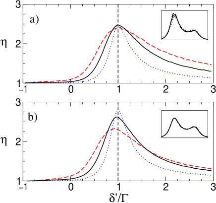
Figure 13: (color online). Spectral dependence of the enhancement factor, for detuning $\delta=\Gamma$ and optical thickness $b=0.5$ (dashed line), $1$ (solid), and $2$ (dotted), in the $h\parallel h$ channel (a) and the scalar case (b). The vertical dashed line displays the position of the elastic $\delta$ peak, which must be filtered out in order to observe an enhancement factor larger than two. The inset shows the power spectrum of the backscattered light (background component), revealing the amplification of the on-resonance peak with respect to the symmetric single-atom spectrum.

On the left hand side, Fig. 11(a) depicts the dependence of the enhancement factor on detuning, for $b=0.5$. As already discussed above, the decrease of $\eta$ with increasing $\delta$ originates from the form of the inelastic power spectrum, which results in a stronger dephasing between reversed paths for larger detuning. Thus, the modification of the enhancement factor with the detuning, keeping fixed the linear optical thickness, is a signature of the nonlinear atomic response and has been experimentally observed in ref. thierry . Let us stress, however, that in the cases shown in Figs. 9 and 11(a) and small detuning, the inelastic component gives a positive contribution to the backscattering enhancement factor. Hence, the observed negative slope of $\eta$ originates from the elastic component, where the nonlinear crossed term is up to two times larger than the ladder, but with negative sign, see Fig. 10(c,d).

In order to observe an enhancement factor larger than two - and thereby demonstrate clearly the effect of interference between three amplitudes - it is therefore necessary to filter out the elastic component. In principle, this can be achieved by means of a spectral filter, i.e. by detecting only photons with a certain frequency $\omega^{\prime}$, different from the laser frequency $\omega$. Thereby, it is possible to measure the spectral dependence of the backscattering enhancement factor, see Fig. 12. Here, the upper (a) and lower (b) half depict the polarized ($h\parallel h$) and scalar case, respectively, for vanishing laser detuning, $\delta=0$. Evidently, the largest values of the enhancement factor are obtained if the final frequency approaches the initial one, since then the dephasing due to different frequencies vanishes. In the scalar case, the value of the enhancement factor in the limit $\delta^{\prime}\to 0$ is completely determined by the relative weights between the one-, two- and three-amplitudes cases shown in Fig. 4, cf. Eq. (38). As evident from the dashed line in Fig. 12(b), already at the rather moderate value $b=0.5$ of the optical thickness, the three-amplitudes case is sufficiently strong in order to increase the maximum enhancement factor above the linear barrier $\eta=2$. With increasing optical thickness (and, if necessary, decreasing saturation parameter, in order to stay in the domain of validity of the perturbative approach, see above), the number of linear scattering events increases, which implies that the three-amplitudes case increasingly dominates, see Fig. 4. In this limit, the enhancement factor approaches the maximum value three. At the same time, however, a larger number of scattering events also leads to stronger dephasing due to different frequencies, $\omega^{\prime}\neq\omega$. This results in a narrower shape of $\eta$ as a function of $\omega^{\prime}$ for larger optical thickness. Nevertheless, as evident from Fig. 12(b), the enhancement factor remains larger than two in a significant range of frequencies $\omega^{\prime}$. The same is true for the polarized case, Fig. 12(a). However, here the enhancement factor cannot exceed the value $2.5$, due to the polarization-induced loss of contrast. At the same time, the optical thickness has less influence on the maximum enhancement factor at $\delta^{\prime}=0$, since single scattering, Fig. 4(a) - and partly also the two-amplitudes case, Fig. 4(b) - are filtered out, so that interference of three amplitudes already prevails at rather small values of the optical thickness.

In Fig. 13, the influence of an initial detuning (here: $\delta=\Gamma$) is displayed. Basically, the above conclusions remain almost equally valid for the detuned case. A small difference is seen in the scalar case, Fig. 13(b), where the maximum of $\eta(\delta^{\prime})$ is found slightly below $\delta$. This is due to the fact that the weight of single scattering increases with increasing $\delta^{\prime}$. Furthermore, the inset reveals that the power spectrum of the backscattered light differs from the single-atom spectrum, Eq. (26), where the two peaks at $\delta^{\prime}=0$ and $\delta^{\prime}=2\delta$ are equally strong. In the multiple scattering case, the on-resonance peak at $\delta^{\prime}=0$ is amplified, since the scattering cross-section is larger for photons on resonance. As already mentioned above, see the discussion of Fig. 9, this increases the total contribution to the detection signal (in the sum over all scattering paths) - especially in the polarized case, where single scattering is filtered out.

V Conclusion

In summary, we have presented a detailed diagrammatic calculation of coherent backscattering of light from a dilute medium composed of weakly saturated two-level atoms. Our theory applies in the perturbative two-photon scattering regime ($s\ll 1$ and $sb^{2}\ll 1$), where at most one nonlinear scattering event occurs. The value of the backscattering enhancement factor is determined by the following three effects: firstly, due to the nonlinearity of the atom-photon interaction, there may be either two or three different amplitudes which interfere in backscattering direction. This implies a maximal enhancement factor between two and three for the nonlinear component, where the value three is approached for large optical thickness. However, since the contribution from nonlinear scattering has a negative sign, the total enhancement factor (linear plus nonlinear elastic and inelastic components) is reduced by the effect of three-amplitudes interference. Only if the elastic component is filtered out, a value larger than two can be observed.

Secondly, a loss of coherence is implied by the change of frequency due to inelastic scattering - like in the case of two atoms wellens . The random frequency change leads to different scattering phases - and hence on average decoherence - between reversed paths. Finally, a further loss of contrast is induced by nonlinear polarization effects - even in the $h\parallel h$ channel, which exhibits ideal contrast in the linear case. Nevertheless, the enhancement factor remains larger than two in certain frequency windows of the inelastic backscattering signal. Thus, it is experimentally possible to clearly identify the effect of interference between three amplitudes - provided a sufficiently narrow spectral filter is at hand.

A natural way to extend this work is to give up the perturbative assumption, and admit more than one nonlinear scattering event. This is necessary in order to describe media with large optical thickness, even at small saturation. Since the number of interfering amplitudes increases if more than two photons are connected by nonlinear scattering events, we expect the occurrence of even larger enhancement factors in the nonperturbative regime - especially in the case of scatterers with positive nonlinearity, i.e. for scatterers whose cross section increases with increasing intensity.

Furthermore, the relation between coherent backscattering and weak localization in the presence of nonlinear scattering remains to be explored. Does a large enhancement of coherent backscattering also imply a strong reduction of nonlinear diffusive transport? If the answer is yes - as it is the case in the linear regime - this implies that wave localization can be facilitated by introducing appropriate nonlinearities.

Appendix A Monte-Carlo simulation

As discussed in Sec. III.3, the incorporation of polarization effects requires to take into account the projection of polarization vectors in the corresponding scalar equations. For the inelastic ladder component, insertion of the polarization term, Eq. (55), into the scalar expression, Eq. (28), yields:

$$\hat{L}_{\rm in}^{(2)}=s\int\frac{d{\bf r}}{A\hat{\ell}}\int d\omega^{\prime}P(\omega^{\prime})\sum_{n,m,l=0}^{\infty}\mathcal{N}^{n+m+l}\times\\ \int_{V}d{\bf u_{1}}\dots d{\bf u_{n}}\quad e^{-u_{1,z}/\hat{\ell}}\left(\prod_{i=1}^{n}\left|\hat{S}_{\omega}\hat{G}_{\omega}({\bf u_{i}},{\bf u_{i+1}})\right|^{2}\right)\\ \int_{V}d{\bf v_{1}}\dots d{\bf v_{m}}\quad e^{-v_{1,z}/\hat{\ell}}\left(\prod_{j=1}^{m}\left|\hat{S}_{\omega}\hat{G}_{\omega}({\bf v_{j}},{\bf v_{j+1}})\right|^{2}\right)\\ \int_{V}d{\bf w_{1}}\dots d{\bf w_{l}}\quad e^{-w_{1,z}/\hat{\ell}^{\prime}}\left(\prod_{k=1}^{l}\left|\hat{S}_{\omega^{\prime}}\hat{G}_{\omega^{\prime}}({\bf w_{k}},{\bf w_{k+1}})\right|^{2}\right)\\ \frac{3}{2}\Pi^{(L)}(\epsilon_{u},\epsilon_{v};\epsilon_{w})\times\begin{cases}1&\text{ if }n=m=0,\\ 2&\text{ if }n>0\text{ or }m>0,\end{cases}$$ (64)

with ${\bf u_{n+1}}={\bf v_{m+1}}={\bf w_{l+1}}={\bf r}$. Furthermore, the polarization vectors are given by:

$$\epsilon_{u} =\Delta_{{\bf u_{n}},{\bf u_{n+1}}}\dots\Delta_{{\bf u_{1}},{\bf u_{2}}}\epsilon_{L},$$ (65)

$$\epsilon_{v} =\Delta_{{\bf v_{m}},{\bf v_{m+1}}}\dots\Delta_{{\bf v_{1}},{\bf v_{2}}}\epsilon_{L},$$

$$\epsilon_{w} =\Delta_{{\bf w_{l}},{\bf w_{l+1}}}\dots\Delta_{{\bf w_{1}},{\bf w_{2}}}\epsilon_{D}.$$

The analogous procedure for the interference component, inserting Eq. (57) into Eq. (33), yields:

$$\hat{C}^{\rm(2,in)}=s\int\frac{d{\bf r}}{A\hat{\ell}}\int d\omega^{\prime}P(\omega^{\prime})\sum_{n,m,l=0}^{\infty}{\mathcal{N}}^{n+m+l}\\ \int_{V}d{\bf u_{1}}\dots d{\bf w_{l}}\quad e^{-u_{1,z}/\hat{\ell}}\left(\prod_{i=1}^{n}\left|\hat{S}_{\omega}\hat{G}_{\omega}({\bf u_{i}},{\bf u_{i+1}})\right|^{2}\right)\\ e^{ikv_{1,z}(n_{\omega}+n^{*}_{\omega^{\prime}})}\left(\prod_{j=1}^{m}\hat{S}_{\omega}\hat{S}^{*}_{\omega^{\prime}}\hat{G}_{\omega}({\bf v_{j}},{\bf v_{j+1}})\hat{G}^{*}_{\omega^{\prime}}({\bf v_{j}},{\bf v_{j+1}})\right)\\ e^{ikw_{1,z}(n^{*}_{\omega}+n_{\omega^{\prime}})}\left(\prod_{k=1}^{l}\hat{S}^{*}_{\omega}\hat{S}_{\omega^{\prime}}\hat{G}^{*}_{\omega}({\bf w_{k}},{\bf w_{k+1}})\hat{G}_{\omega^{\prime}}({\bf w_{k}},{\bf w_{k+1}})\right)\\ \frac{3}{2}\Pi^{(C)}(\epsilon_{u},\epsilon_{v},\tilde{\epsilon}_{w},\epsilon_{w},\tilde{\epsilon}_{v})\times\begin{cases}0,&\text{if }m=l=0,\\ 2,&\text{if }n=m=0,\quad l>0\\ 2,&\text{if }n=l=0,\quad m>0,\\ 4,&\text{otherwise}\end{cases}$$ (66)

with the polarization vectors of the ‘reversed’ photons:

$$\tilde{\epsilon_{v}} =\Delta_{{\bf v_{m}},{\bf v_{m+1}}}\dots\Delta_{{\bf v_{1}},{\bf v_{2}}}\epsilon_{D},$$ (67)

$$\tilde{\epsilon}_{w} =\Delta_{{\bf w_{l}},{\bf w_{l+1}}}\dots\Delta_{{\bf w_{1}},{\bf w_{2}}}\epsilon_{L}.$$

The elastic nonlinear scattering components follow simply by inserting $-2\delta(\omega^{\prime}-\omega)$ instead of the inelastic power spectrum $P(\omega^{\prime})$ in the above Eqs. (64,66).

The nonlinear propagation term is obtained by inserting Eq. (58) into Eq. (44):

$$\hat{L}_{\rm el}^{\rm(2,prop)}=s\sum_{n=1}^{\infty}{\mathcal{N}}^{n}\int_{V}d{\bf u_{1}}\dots d{\bf u_{n}}\quad e^{-(u_{1,z}+u_{n,z})/\hat{\ell}}\\ \left(\prod_{i=1}^{n}\left|\hat{S}_{\omega}\hat{G}_{\omega}({\bf u_{i}},{\bf u_{i+1}})\right|^{2}\right)\sum_{m=1}^{\infty}{\mathcal{N}}^{m-1}\int_{V}d{\bf v}_{1}\dots d{\bf v}_{m-1}\\ \sum_{l=0}^{n}\int_{\bf u_{l}}^{\bf u_{l+1}}\frac{d{\bf v_{m}}}{\hat{\ell}}\quad e^{-v_{1,z}/\hat{\ell}}\left(\prod_{i=1}^{m-1}\left|\hat{S}_{\omega}\hat{G}_{\omega}({\bf v_{i}},{\bf v_{i+1}})\right|^{2}\right)\\ \Pi^{(L,\text{prop})}(\epsilon_{1},\epsilon_{v},\epsilon_{3})\times\begin{cases}1&\text{if }m=l=0,\\ 2&\text{otherwise},\end{cases}$$ (68)

Here, the nonlinear event takes place between $\bf u_{l}$ and $\bf u_{l+1}$. Correspondingly, $\int_{\bf u_{l}}^{\bf u_{l+1}}$ denotes the one-dimensional integral on a straight line between these points, and ${\bf u_{0}}={\bf u_{1}}-u_{1,z}{\bf e_{z}}$ and ${\bf u_{n+1}}={\bf u_{n}}-u_{n,z}{\bf e_{z}}$ are defined as the points where the photon enters or leaves the medium, respectively. The three cases Fig. 5(a,b,c) correspond to $0<l<n$, $l=n$, and $l=0$, respectively. The polarization vectors $\epsilon_{1}$ and $\epsilon_{3}$ participating in the nonlinear event, cf. Fig. 8, are obtained as:

$$\epsilon_{1} =\Delta_{{\bf u_{l+1}},{\bf u_{l}}}\dots\Delta_{{\bf u_{2}},{\bf u_{1}}}\epsilon_{L},$$ (69)

$$\epsilon_{3} =\Delta_{{\bf u_{l}},{\bf u_{l+1}}}\dots\Delta_{{\bf u_{n-1}},{\bf u_{n}}}\epsilon_{D}.$$

Finally, to obtain the interference component $\hat{C}^{\rm(2,prop)}_{\rm el}$, the last term in Eq. (68) must be replaced by:

$$\Pi^{(L,\text{prop})}(\epsilon_{1},\epsilon_{v},\epsilon_{3})\times\begin{cases}2&\text{if }n>1,(m,l)\neq(0,0),\\ 1&\text{if }n>1,m=l=0,\\ 0&\text{otherwise}\end{cases}+\\ \Pi^{(C,\text{prop})}(\epsilon_{1},\epsilon_{v},\epsilon_{3},\tilde{\epsilon}_{v},\tilde{\epsilon}_{3})\times\begin{cases}4&\text{if }l=0,n>1,m>0,\\ 2&\text{if }l=0,n=1,m>0,\\ 2&\text{if }0<l<n,\\ 0&\text{otherwise},\end{cases}$$ (70)

with

$$\tilde{\epsilon}_{3}=\Delta_{{\bf u_{l}},{\bf u_{l+1}}}\dots\Delta_{{\bf u_{n-1}},{\bf u_{n}}}\epsilon_{L}.$$ (71)

The first term, $\Pi^{(L,{\rm prop})}$, equals the ladder component minus single scattering ($n=1$), whereas the second one, $\Pi^{(C,{\rm prop})}$, describes the additional crossed diagrams shown in Fig. 6(d-f). Here, the case $0<l<n$ corresponds to Fig. 6(d), where the nonlinearity occurs between two scattering events. The remaining diagrams, Fig. 6(e,f), correspond to $l=0$. Here, the case $m=0$ (‘pump photon from the coherent mode’) does not contribute, since then the diagrams Fig. 6(e,f) are identical to Fig. 6(b,c). Furthermore, if $n=1$ (‘probe photon singly scattered’), the two diagrams Fig. 6(e) and (f) become identical. In this case, we obtain a factor $2$, whereas the sum of diagram (e) plus diagram (f) yields $2+2=4$ in the case $n>1$.

Numerically, we solve the above integrals by a Monte-Carlo method. Here, we proceed as follows: for Eqs. (64,66), at first position ${\bf r}$ and frequency $\omega_{D}$ of the inelastic scattering event are chosen randomly. Starting from ${\bf r}$, three photons are launched, two with frequency $\omega_{L}$ and one with frequency $\omega_{D}$. After each scattering event, the length $r$ of the next propagation step is determined randomly according to the distribution $P(r)=\exp(-r/\ell)/\ell$, whereas the direction is chosen uniformly. After all photons have left the medium, the triple sum over $n$, $m$, and $l$ is performed, taking into account the projection of the polarization vectors. For the nonlinear propagation term, Eq. (68), at first the probe photon (path: $\bf u_{1},\dots,{\bf u_{n}}$) is propagated, starting in the laser mode ${\bf k_{L}},\epsilon_{L}$. Then, the pump photon is launched from a randomly chosen position ${\bf v_{m}}$ on the path of the probe photon. Finally, the projection of polarization vectors is performed separately for each given path.

References

- (1) A. Schuster, Astrophys. J. 21, 1 (1905).
- (2) D. Mihalas, Stellar Atmospheres, 2nd Ed, Freeman, San Francisco (1978).
- (3) S. Chandrasekhar, Radiative Transfer, Dover, New York (1960).
- (4) H.C. van de Hulst, Multiple Light Scattering, vols. I and II, Academic Press, New York (1980).
- (5) T. Holstein, Phys. Rev. 72, 1212 (1947) ; T. Holstein, Phys. Rev. 83, 1159 (1951).
- (6) A.F. Molisch and B.P. Oehry, Radiation trapping in atomic vapors, Oxford Science Publications, Oxford University Press, New York (1998).
- (7) Laser Speckle and Related Phenomena, Ed. C. Dainty, Topics in Applied Physics 9, Springer Verlag, Berlin (1984).
- (8) P.W. Anderson, Phys. Rev. 109, 1492 (1958).
- (9) J.S. Langer and T. Neal, Phys. Rev. Lett. 16, 984 (1966).
- (10) G. Bergmann, Phys. Rep. 107, 1 (1984).
- (11) Mesoscopic quantum physics, Proceedings of the Les Houches Summer School, Session LXI, E. Akkermans and G. Montambaux and J. L. Pichard and J. Zinn-Justin eds, North Holland, Elsevier Science B. V., Amsterdam (1995).
- (12) Physique mésoscopique des électrons et des photons, E. Akkermans and G. Montambaux, EDP Sciences, CNRS Editions (2004). An english translation is in preparation.
- (13) A. Akkermans et G. Montambaux, J. Opt. Soc. Am. B 21, 101 (2004) and references therein.
- (14) F. Scheffold and G. Maret, Phys. Rev. Lett. 81, 5800 (1998).
- (15) D.S. Wiersma, P. Bartolini, A. Lagendijk and R. Righini, Nature 390, 671 (1997).
- (16) G. Maret, Current Opinion in Colloid and Interface Science 2, 251 (1997).
- (17) M. P. van Albada and A. Lagendijk, Phys. Rev. Lett. 55, 2692 (1985); P. E. Wolf and G. Maret, Phys. Rev. Lett. 55, 2696 (1985).
- (18) E. Akkermans, P.E. Wolf, R. Maynard and G. Maret, J. Phys. (Paris) 49, 77 (1988).
- (19) B. van Tiggelen and R. Maynard, in Waves in Random and other complex media, L. Burridge, G. Papanicolaou and L. Pastur eds., Springer, vol. 96, p247 (1997).
- (20) V.M. Agranovich and V.E. Kravtsov, Phys. Rev. B 43, 13691 (1991)
- (21) A. Heiderich, R. Maynard and B.A. van Tiggelen, Opt. Comm. 115, 392 (1995).
- (22) G. Labeyrie, F. de Tomasi, J.-C. Bernard, C. A. Müller, C. Miniatura, and R. Kaiser, Phys. Rev. Lett. 83, 5266 (1999).
- (23) T. Jonckheere, C. A. Müller, R. Kaiser, C. Miniatura and D. Delande, Phys. Rev. Lett. 85, 4269 (2000).
- (24) C. A. Müller, T. Jonckheere, C. Miniatura, and D. Delande, Phys. Rev. A 64, 053804 (2001).
- (25) C. A. Müller and C. Miniatura, J. Phys. A 35, 10163 (2002).
- (26) D.V. Kupriyanov, I.M. Sokolov and M.D. Havey, Optics Comm. 243, 165 (2004).
- (27) V.S. Lethokov, Sov. Phys. JETP 26, 835 (1968).
- (28) N. M. Lawandy, R. M. Balachandran, A. S. L. Gomes, and E. Sauvain, Nature 368, 436 (1994).
- (29) H. Cao, Y. G. Zhao, S. T. Ho, E. W. Seelig, Q. H. Wang, and R. P. H. Chang, Phys. Rev. Lett.82, 2278 (1999).
- (30) H. Cao, Waves Random Media 13, R1 (2003) and references therein.
- (31) T. Wellens, B. Grémaud, D. Delande, and C. Miniatura, Phys. Rev. E 71, 055603(R) (2005).
- (32) T. Wellens, B. Grémaud, D. Delande, and C. Miniatura, Phys. Rev. A 70, 023817 (2004).
- (33) V. Shatokhin, C.A. Müller, and A. Buchleitner, Phys. Rev. Lett. 94, 043603 (2005).
- (34) B. Grémaud, T. Wellens, D. Delande and Ch. Miniatura, submitted to Phys. Rev. A (2005).
- (35) A. Lagendijk and B.A. van Tiggelen, Phys. Rep. 270, 143 (1996).
- (36) G. Labeyrie, Ch. Miniatura and R. Kaiser, Phys. Rev. A 64, 033402 (2001).
- (37) D. Wiersma, M. P. van Albada, B. A. van Tiggelen, and A. Lagendijk, Phys. Rev. Lett 74, 4193 (1995).
- (38) C. Cohen-Tannoudji, J. Dupont-Roc, and G. Grynberg, Atom-Photon Interactions (Wiley, New York, 1992).
- (39) J. W. Goodman, in Laser speckle and related phenomena, ed. by J. C. Dainty (Springer, Berlin, 1984).
- (40) T. Chanelière, D. Wilkowski, Y. Bidel, R. Kaiser, and C. Miniatura, Phys. Rev. E 70, 036602 (2004).
- (41) S. Balik, P. Kulatunga, C.I. Sukenik, M.D. Havey, D.V. Kupriyanov and I.M. Sokolov, submitted to Journal of Modern Optics (Proceedings of PQE2005).
- (42) In our article wellens2 , the statement in the paragraph following Eq.(11) is thus wrong and so are the numerical results depicted in Fig. 3. The corrected figure can be obtained by sending an email to Thomas.Wellens@spectro.jussieu.fr
- (43) S. E. Skipetrov and R. Maynard, Phys. Rev. Lett 85, 736 (2000).