Born expansion of the Casimir-Polder interaction of a ground-state atom with dielectric bodies

Abstract

Within leading-order perturbation theory, the Casimir-Polder potential of a ground-state atom placed within an arbitrary arrangement of dispersing and absorbing linear bodies can be expressed in terms of the polarizability of the atom and the scattering Green tensor of the body-assisted electromagnetic field. Based on a Born series of the Green tensor, a systematic expansion of the Casimir-Polder potential in powers of the electric susceptibilities of the bodies is presented. The Born expansion is used to show how and under which conditions the Casimir-Polder force can be related to microscopic many-atom van der Waals forces, for which general expressions are presented. As an application, the Casimir-Polder potentials of an atom near a dielectric ring and an inhomogeneous dielectric half space are studied and explicit expressions are presented that are valid up to second order in the susceptibility.

PACS 12.20.-m Quantum electrodynamics – 34.50.Dy Interactions of atoms and molecules with surfaces; photon and electron emission; neutralization of ions – 34.20.-b Interatomic and intermolecular potentials and forces, potential energy surfaces for collisions – 42.50.Nn Quantum optical phenomena in absorbing, dispersive and conducting media

1 Introduction

The forces of electromagnetic origin that arise between electrically neutral, unpolarized but polarizable objects are commonly known as dispersion forces Dzyaloshinskii61 ; Langbein74 ; Mahanty76 ; Hinds91 ; Milonni94 . They were first addressed within the context of quantum electrodynamics (QED) by Casimir and Polder Casimir48 ; Casimir48b , who showed that they may be attributed to the vacuum fluctuations of the electromagnetic field. In accordance with the different nature of the interacting objects, one may distinguish between three types of dispersion forces, namely the forces between atoms—in the following referred to as van der Waals (vdW) forces, the forces between atoms and macroscopic bodies—in the following referred to as Casimir-Polder (CP) forces, and the forces between macroscopic bodies—in the following referred to as Casimir forces.

Dispersion forces play a major role in the understanding of many phenomena, and they can be a useful or disturbing factor in modern applications. Apart from being crucial for the understanding of many structures and processes in biochemistry Nelson02 , they are responsible for the remarkable climbing skills of some gecko Autumn02 and spider species Kesel04 ; the construction of atomic-force microscopes is essentially based on dispersion forces Binnig86 , while they are also responsible for the problem of sticking in nanotechnology Henkel04 . In particular, CP forces between atoms and macroscopic bodies are needed for an understanding of the adsorption of atoms and molecules to surfaces Bruch83 ; they can be used in atom optics to construct atomic mirrors Shimizu02 , while they have also been found to severely limit the lifetime of atoms stored on atom chips Lin04 .

The study of CP forces which were first predicted for the idealized situation of a ground-state atom interacting with a perfectly conducting plate Casimir48 has since been greatly extended. Various planar geometries like the semi-infinite half space McLachlan63 ; McLachlan63b ; Tiko93 ; Enderlein99 , plates of finite thickness Zhou95 , two-layered plates Wylie84 or planar cavities Zhou95 ; Jhe91 have been treated, the most general planar geometry being the planar multilayer system with an arbitrary number of layers Buhmann05 ; Buhmann05b . Systems with spherical Marvin82 ; Girard89 or cylindrical symmetries Marvin82 ; Boustimi02 have also been considered. It should be mentioned that some theoretical approaches (in particular, those based on normal-mode quantization, e.g., Refs. Casimir48 ; Tiko93 ; Enderlein99 ; Zhou95 ; Jhe91 ; Marvin82 ) require a separate treatment for each specific geometry, whereas others (in particular, the methods based on linear response theory, e.g., Refs. McLachlan63 ; McLachlan63b ; Wylie84 ; Girard89 ; Boustimi02 ) lead to general expressions that are geometry-independent.

Recently, the problem has been studied within the frame of macroscopic QED in dispersing and absorbing media and an exact derivation of a general expression for the CP force has been given Buhmann05 ; Buhmann04 ; Buhmann04b . Although the problem of calculating CP forces (or equivalently, the respective CP potentials) is thus formally solved, explicit evaluation requires knowledge of the (classical) Green tensor for the body-assisted electromagnetic field, which is (analytically) available only for a very limited class of geometries. In particular, inhomogeneous bodies or bodies of exotic shapes have not yet been treated. Nevertheless, it shall be demonstrated in this paper that the general solution—in combination with a Born expansion of the Green tensor—may serve as a starting point for the systematic study of a wide class of geometries.

Furthermore, the Born expansion helps making general statements about two fundamental issues regarding CP forces. First, it may answer the question of whether and to what extent CP forces are additive. Second, it can be used to clarify the microscopic origin of CP forces. It is known that up to linear order in the electric susceptibility the force between an atom and a macroscopic body that may be regarded composed of atom-like constituents can be obtained by summation of two-atom (microscopic) vdW forces Milonni94 ; Lifshitz56 ; an analogous relation between the Casimir force and CP forces can be established Lifshitz56 ; Parsegian74 ; Schwinger78 ; Mil92 ; Kup92 ; Barton01 ; Raa05 . It is also known that pairwise summation fails at higher order in the susceptibility Renne67 ; Milonni92b , where many-atom interactions begin to play a role Axilrod43 ; Aub60 ; Power85 ; Power94 ; Cirone96 ; in fact, it has been shown that an infinite series of many-atom interactions must be included in order to derive the CP force between an atom and a semi-infinite dielectric half space microscopically Renne67 .

The article is organized as follows. In Sec. 2 the Born expansion of the CP potential of an atom placed within an arbitrary arrangement of locally, linearly, and causally responding isotropic dielectric bodies is given. The results are then used to elucidate the relation to microscopic descriptions (Sec. 3), and to study some specific geometries (Sec. 4). Finally, a summary is given in Sec. 5.

2 Born expansion

Consider a neutral, non-polar, ground-state atomic system $A$ such as an atom or a molecule (briefly referred to as atom in the following) at position $\vec{r}_{A}$ which is placed in a free-space region within an arbitrary arrangement of linear dielectric bodies. The system of bodies is characterized by the (relative) permittivity $\varepsilon(\vec{r},\omega)$, which is a spatially varying, complex-valued function of frequency, with the Kramers-Kronig relations being satisfied. Within leading-order perturbation theory, the CP force on the atom due to the presence of the bodies can be derived from the CP potential (see, e.g., Ref. Buhmann04 )

$$U_{A}(\vec{r}_{A})=\frac{\hbar\mu_{0}}{2\pi}\int_{0}^{\infty}\mathrm{d}u\,u^{2}\alpha_{A}(iu)\,\mathrm{Tr}\,\mathsf{G}^{(1)}(\vec{r}_{A},\vec{r}_{A},iu)$$ (1)

according to

$$\vec{F}_{A}(\vec{r}_{A})=-\bm{\nabla}_{\!\!A}U_{A}(\vec{r}_{A})$$ (2)

($\bm{\nabla}_{\!\!A}$ $\!\equiv$ $\!\bm{\nabla}_{\!\vec{r}_{A}}$). In Eq. (1),

$$\alpha_{A}(\omega)=\lim_{\epsilon\to 0}\frac{2}{3\hbar}\sum_{n}\frac{\omega_{n0}^{A}|\vec{d}^{A}_{0n}|^{2}}{(\omega_{n0}^{A})^{2}-\omega^{2}-i\omega\epsilon}$$ (3)

is the ground-state polarizability of the atom in lowest order of perturbation theory [$\omega_{n0}^{A}$ $\!\equiv$ $\!(E_{n}^{A}$ $\!-$ $\!E_{0}^{A})/\hbar$, (bare) atomic transition frequencies; $\vec{d}^{A}_{0n}$ $\!\equiv$ $\!\langle 0_{A}|\hat{\vec{d}}_{A}|n_{A}\rangle$, electric-dipole transition matrix elements of the atom], and $\mathsf{G}^{(1)}(\vec{r},\vec{r}^{\prime},iu)$ is the scattering part of the classical Green tensor of the body-assisted electromagnetic field,

$$\mathsf{G}(\vec{r},\vec{r}^{\prime},\omega)=\mathsf{G}^{(0)}(\vec{r},\vec{r}^{\prime},\omega)+\mathsf{G}^{(1)}(\vec{r},\vec{r}^{\prime},\omega)$$ (4)

[$\mathsf{G}^{(0)}(\vec{r},\vec{r}^{\prime},\omega)$, vacuum part], which is the solution to the equation

$$\biggl{[}\bm{\nabla}\times\bm{\nabla}\times-\frac{\omega^{2}}{c^{2}}\,\varepsilon(\vec{r},\omega)\biggr{]}\mathsf{G}(\vec{r},\vec{r}^{\prime},\omega)=\delta(\vec{r}-\vec{r}^{\prime})\mathsf{I}$$ (5)

($\mathsf{I}$, unit tensor) together with the boundary condition

$$\mathsf{G}(\vec{r},\vec{r}^{\prime},\omega)\to 0\quad\mbox{for}\quad|\vec{r}-\vec{r}^{\prime}|\to\infty.$$ (6)

Suppose now that

$$\varepsilon(\vec{r},\omega)=\overline{\varepsilon}(\vec{r},\omega)+\chi(\vec{r},\omega),$$ (7)

with the Green tensor $\overline{\mathsf{G}}(\vec{r},\vec{r}^{\prime},\omega)$, which is the solution to

$$\biggl{[}\bm{\nabla}\times\bm{\nabla}\times-\frac{\omega^{2}}{c^{2}}\,\overline{\varepsilon}(\vec{r},\omega)\biggr{]}\overline{\mathsf{G}}(\vec{r},\vec{r}^{\prime},\omega)=\delta(\vec{r}-\vec{r}^{\prime})\mathsf{I},$$ (8)

being known. A (formal) solution to Eq. (5) can then be given by the Born series

$$\mathsf{G}(\vec{r},\vec{r}^{\prime},\omega)=\overline{\mathsf{G}}(\vec{r},\vec{r}^{\prime},\omega)$$

$$\hskip 4.30554pt+\sum_{k=1}^{\infty}\Bigl{(}\frac{\omega}{c}\Bigr{)}^{2k}\Biggl{[}\prod_{j=1}^{k}\int\mathrm{d}^{3}s_{j}\,\chi(\vec{s}_{j},\omega)\Biggr{]}$$

$$\quad\times\overline{\mathsf{G}}(\vec{r},\vec{s}_{1},\omega)\cdot\overline{\mathsf{G}}(\vec{s}_{1},\vec{s}_{2},\omega)\cdots\overline{\mathsf{G}}(\vec{s}_{k},\vec{r}^{\prime},\omega),$$ (9)

as can be easily verified using Eq. (8) together with

$$\biggl{[}\bm{\nabla}\!\times\!\bm{\nabla}\!\times\!-\frac{\omega^{2}}{c^{2}}\,\overline{\varepsilon}(\vec{r},\omega)\biggr{]}\sum_{k=1}^{\infty}\Bigl{(}\frac{\omega}{c}\Bigr{)}^{2k}\Biggl{[}\prod_{j=1}^{k}\int\mathrm{d}^{3}s_{j}\,\chi(\vec{s}_{j},\omega)\Biggr{]}$$

$$\quad\times\overline{\mathsf{G}}(\vec{r},\vec{s}_{1},\omega)\cdot\overline{\mathsf{G}}(\vec{s}_{1},\vec{s}_{2},\omega)\cdots\overline{\mathsf{G}}(\vec{s}_{k},\vec{r}^{\prime},\omega)$$

$$\qquad=\Bigl{(}\frac{\omega}{c}\Bigr{)}^{2}\chi(\vec{r},\omega)\mathsf{G}(\vec{r},\vec{r}^{\prime},\omega).$$ (10)

Combining Eqs. (1), (4), and (2), we find that the CP potential can be expanded as

$$U_{A}(\vec{r}_{A})=\overline{U}_{A}(\vec{r}_{A})+\sum_{k=1}^{\infty}\Delta_{k}U_{A}(\vec{r}_{A}),$$ (11)

where

$$\overline{U}_{A}(\vec{r}_{A})=\frac{\hbar\mu_{0}}{2\pi}\int_{0}^{\infty}\mathrm{d}u\,u^{2}\alpha_{A}(iu)\,\mathrm{Tr}\,\overline{\mathsf{G}}^{(1)}(\vec{r}_{A},\vec{r}_{A},iu)$$ (12)

is the CP potential due to $\overline{\varepsilon}(\vec{r},\omega)$, and

$$\Delta_{k}U_{A}(\vec{r}_{A})=\frac{(-1)^{k}\hbar\mu_{0}}{2\pi c^{2k}}$$

$$\hskip 4.30554pt\times\int_{0}^{\infty}\mathrm{d}u\,u^{2k+2}\alpha_{A}(iu)\Biggl{[}\prod_{j=1}^{k}\int\mathrm{d}^{3}s_{j}\,\chi(\vec{s}_{j},iu)\Biggr{]}$$

$$\hskip 4.30554pt\times\mathrm{Tr}\bigl{[}\overline{\mathsf{G}}(\vec{r}_{A},\vec{s}_{1},iu)\cdot\overline{\mathsf{G}}(\vec{s}_{1},\vec{s}_{2},iu)\cdots\overline{\mathsf{G}}(\vec{s}_{k},\vec{r}_{A},iu)\bigr{]}$$ (13)

is the contribution to the potential that is of $k$th order in $\chi(\vec{r},\omega)$. The Born expansion of the CP potential as given by Eqs. (11)–(2) can be used to (systematically) calculate the potential in scenarios where a basic arrangement of bodies for which the Green tensor is known is (weakly) disturbed, e.g., by additional bodies or inhomogeneities such as surface roughness.

Let us apply Eq. (11)–(2) to the case of arbitrarily shaped, weakly dielectric bodies, so that we may let $\overline{\varepsilon}(\mathbf{r},\omega)$ $\!\equiv$ $\!1$, and hence

$$U_{A}(\vec{r}_{A})=\sum_{k=1}^{\infty}\Delta_{k}U_{A}(\vec{r}_{A}),$$ (14)

where $\Delta_{k}U_{A}(\vec{r}_{A})$ is given by Eq. (2), with

$$\overline{\mathsf{G}}(\vec{r},\vec{r}^{\prime},iu) =\mathsf{G}_{\mathrm{V}}(\vec{r},\vec{r}^{\prime},iu)$$

$$=\frac{1}{4\pi}\biggl{[}\mathsf{I}-\Bigl{(}\frac{c}{u}\Bigr{)}^{2}\bm{\nabla}\otimes\bm{\nabla}\biggr{]}\frac{e^{-\frac{u\rho}{c}}}{\rho}$$

$$=\frac{1}{3}\Bigl{(}\frac{c}{u}\Bigr{)}^{2}\delta(\bm{\rho})\mathsf{I}+\mathsf{H}_{\mathrm{V}}(\vec{r},\vec{r}^{\prime},iu)$$ (15)

being the vacuum Green tensor (see, e.g., Ref. Knoll01 ), where

$$\mathsf{H}_{\mathrm{V}}(\vec{r},\vec{r}^{\prime},iu)=\frac{c^{2}e^{-\frac{u\rho}{c}}}{4\pi u^{2}\rho^{3}}\biggl{[}a\Bigl{(}\frac{u\rho}{c}\Bigr{)}\mathsf{I}-b\Bigl{(}\frac{u\rho}{c}\Bigr{)}\hat{\bm{\rho}}\otimes\hat{\bm{\rho}}\biggr{]},$$ (16)

$$a(x) =1+x+x^{2},$$ (17)

$$b(x) =3+3x+x^{2}$$ (18)

($\bm{\rho}$ $\!\equiv$ $\!\vec{r}-\vec{r}^{\prime}$; $\rho$ $\!\equiv$ $\!|\bm{\rho}|$; $\hat{\bm{\rho}}$ $\!\equiv$ $\!\bm{\rho}/\rho$). Combining Eqs. (2) and (2) [together with Eqs. (16)–(18)], one easily finds that to linear order in $\chi$ the CP potential reads

$$U_{A}(\vec{r}_{A}) =\Delta_{1}U_{A}(\vec{r}_{A})=-\frac{\hbar}{32\pi^{3}\varepsilon_{0}}\int_{0}^{\infty}\mathrm{d}u\,\alpha_{A}(iu)$$

$$\quad\times\int\mathrm{d}^{3}s\,\chi(\vec{s},iu)\,\frac{g_{2}(u|\vec{r}_{A}-\vec{s}|/c)}{|\vec{r}_{A}-\vec{s}|^{6}},$$ (19)

where

$$g_{2}(x)=2e^{-2x}(3+6x+5x^{2}+2x^{3}+x^{4}).$$ (20)

In this approximation the CP force is simply a volume integral over attractive central forces, as is seen from

$$\bm{\nabla}\biggl{[}\frac{g_{2}(ur/c)}{r^{6}}\biggr{]}=-\frac{\hat{\vec{r}}}{r^{7}}\bigl{[}6g_{2}(ur/c)-(ur/c)g^{\prime}_{2}(ur/c)\bigr{]}$$

$$\quad=-\frac{4\hat{\vec{r}}}{r^{7}}\bigl{[}e^{-2x}(9\!+\!18x\!+\!16x^{2}\!+\!8x^{3}$$

$$\quad\hskip 34.44434pt+\!3x^{4}\!+\!x^{5})\bigr{]}_{x=ur/c}$$ (21)

($r$ $\!\equiv$ $\!|\vec{r}|$, $\hat{\vec{r}}$ $\!\equiv$ $\!\vec{r}/r$).

In the retarded (long-distance) limit, i.e.,

$$r_{-}\gg\frac{c}{\omega_{A}^{-}}\,,\quad r_{-}\gg\frac{c}{\omega_{\mathrm{M}}^{-}}\,,$$ (22)

where $r_{-}$ $\!\equiv$ $\min\{|\vec{r}_{A}-\vec{s}|:\chi(\vec{s})\neq 0\}$ is the minimum distance of the atom to any of the bodies, $\omega_{A}^{-}$ $\!\equiv$ $\!\mathrm{min}\{\omega_{n0}^{A}|n$ $\!=$ $\!1,2,\ldots\}$ is the lowest atomic transition frequency, and $\omega_{\mathrm{M}}^{-}$ is the lowest resonance frequency of the dielectric material, the exponential factor in $g_{2}(x)$ effectively limits the $u$-integral in Eq. (2) to a region where

$$\alpha_{A}(iu)\simeq\alpha_{A}(0),\ \chi(\vec{s},iu)\simeq\chi(\mathbf{s},0),$$ (23)

so Eq. (2) reduces to

$$\Delta_{1}U_{A}(\vec{r}_{A}) = -\frac{\hbar c\alpha_{A}(0)}{32\pi^{3}\varepsilon_{0}}\int\mathrm{d}^{3}s\,\frac{\chi(\mathbf{s},0)}{|\vec{r}_{A}-\vec{s}|^{7}}\int_{0}^{\infty}\mathrm{d}x\,g_{2}(x)$$ (24)

$$= -\frac{23\hbar c\alpha_{A}(0)}{64\pi^{3}\varepsilon_{0}}\int\mathrm{d}^{3}s\,\frac{\chi(\vec{s},0)}{|\vec{r}_{A}-\vec{s}|^{7}}\,.$$

In the nonretarded (short-distance) limit, i.e.,

$$r_{+}\ll\frac{c}{\omega_{A}^{+}}\quad\mathrm{and/or}\quad r_{+}\ll\frac{c}{\omega_{\mathrm{M}}^{+}}\,,$$ (25)

where $r_{+}$ $\!\equiv$ $\max\{|\vec{r}_{A}-\vec{s}|:\chi(\vec{s})\neq 0\}$ is the maximum distance of the atom to any body part, $\omega_{A}^{+}$ $\!\equiv$ $\!\mathrm{max}\{\omega_{n0}^{A}|n$ $\!=$ $\!1,2,\ldots\}$ is the highest atomic transition frequency, and $\omega_{\mathrm{M}}^{+}$ is the highest resonance frequency of the dielectric material, the factors $\alpha_{A}(iu)$ and $\chi(\vec{s},iu)$ effectively limit the $u$-integral in Eq. (2) to a region where $x$ $\!=$ $\!u|\vec{r}_{A}-\vec{s}|/c$ $\!\ll$ $\!1$, so we may set

$$g_{2}(x)\simeq g_{2}(0)=6,$$ (26)

resulting in

$$\Delta_{1}U_{A}(\vec{r}_{A})=-\frac{3\hbar}{16\pi^{3}\varepsilon_{0}}\int_{0}^{\infty}\!\mathrm{d}u\,\alpha_{A}(iu)\int\mathrm{d}^{3}s\,\frac{\chi(\vec{s},iu)}{|\vec{r}_{A}-\vec{s}|^{6}}\,.$$ (27)

The second-order contribution $\Delta_{2}U_{A}(\vec{r}_{A})$ can be separated into a single-point term and a two-point correlation term,

$$\Delta_{2}U_{A}(\vec{r}_{A})=\Delta_{2}^{1}U_{A}(\vec{r}_{A})+\Delta_{2}^{2}U_{A}(\vec{r}_{A}),$$ (28)

as can be seen from Eqs. (2) and (2) for $k$ $\!=$ $\!2$. The single-point term

$$\Delta_{2}^{1}U_{A}(\vec{r}_{A}) =\frac{\hbar}{96\pi^{3}\varepsilon_{0}}\int_{0}^{\infty}\mathrm{d}u\,\alpha_{A}(iu)$$

$$\quad\times\int\mathrm{d}^{3}s\,\chi^{2}(\vec{s},iu)\,\frac{g_{2}(u|\vec{r}_{A}-\vec{s}|/c)}{|\vec{r}_{A}-\vec{s}|^{6}}\,,$$ (29)

which arises from the $\delta$-function in Eq. (2), differs from the first-order contribution $\Delta_{1}U_{A}(\vec{r}_{A})$ according to

$$\chi(\vec{r},\omega)\mapsto-\frac{1}{3}\chi^{2}(\vec{r},\omega),$$ (30)

hence its asymptotic retarded and nonretarded forms can be obtained by applying the replacement (30) to Eqs. (24) and (27), respectively.

The two-point correlation term is derived to be

$$\Delta_{2}^{2}U_{A}(\vec{r}_{A}) =\frac{\hbar}{128\pi^{4}\varepsilon_{0}}\int_{0}^{\infty}\mathrm{d}u\,\alpha_{A}(iu)\int\mathrm{d}^{3}s_{1}\,\chi(\vec{s}_{1},iu)$$

$$\quad\times\int\mathrm{d}^{3}s_{2}\,\chi(\vec{s}_{2},iu)\,\frac{g_{3}(u,\bm{\alpha},\bm{\beta},\bm{\gamma})}{\alpha^{3}\beta^{3}\gamma^{3}},$$ (31)

where

$$g_{3}(u,\bm{\alpha},\bm{\beta},\bm{\gamma})=e^{-u(\alpha+\beta+\gamma)/c}\biggl{[}3a\Bigl{(}\frac{u\alpha}{c}\Bigr{)}a\Bigl{(}\frac{u\beta}{c}\Bigr{)}a\Bigl{(}\frac{u\gamma}{c}\Bigr{)}$$

$$-b\Bigl{(}\frac{u\alpha}{c}\Bigr{)}a\Bigl{(}\frac{u\beta}{c}\Bigr{)}a\Bigl{(}\frac{u\gamma}{c}\Bigr{)}\!-a\Bigl{(}\frac{u\alpha}{c}\Bigr{)}b\Bigl{(}\frac{u\beta}{c}\Bigr{)}a\Bigl{(}\frac{u\gamma}{c}\Bigr{)}$$

$$-a\Bigl{(}\frac{u\alpha}{c}\Bigr{)}a\Bigl{(}\frac{u\beta}{c}\Bigr{)}b\Bigl{(}\frac{u\gamma}{c}\Bigr{)}\!+b\Bigl{(}\frac{u\alpha}{c}\Bigr{)}b\Bigl{(}\frac{u\beta}{c}\Bigr{)}a\Bigl{(}\frac{u\gamma}{c}\Bigr{)}(\hat{\bm{\alpha}}\!\cdot\!\hat{\bm{\beta}})^{2}$$

$$+a\Bigl{(}\frac{u\alpha}{c}\Bigr{)}b\Bigl{(}\frac{u\beta}{c}\Bigr{)}b\Bigl{(}\frac{u\gamma}{c}\Bigr{)}(\hat{\bm{\beta}}\!\cdot\!\hat{\bm{\gamma}})^{2}$$

$$+b\Bigl{(}\frac{u\alpha}{c}\Bigr{)}a\Bigl{(}\frac{u\beta}{c}\Bigr{)}b\Bigl{(}\frac{u\gamma}{c}\Bigr{)}(\hat{\bm{\gamma}}\!\cdot\!\hat{\bm{\alpha}})^{2}$$

$$-b\Bigl{(}\frac{u\alpha}{c}\Bigr{)}b\Bigl{(}\frac{u\beta}{c}\Bigr{)}b\Bigl{(}\frac{u\gamma}{c}\Bigr{)}(\hat{\bm{\alpha}}\!\cdot\!\hat{\bm{\beta}})(\hat{\bm{\beta}}\!\cdot\!\hat{\bm{\gamma}})(\hat{\bm{\gamma}}\!\cdot\!\hat{\bm{\alpha}})\biggr{]},$$ (32)

with the abbreviations

$$\bm{\alpha}\equiv\vec{r}_{A}-\vec{s}_{1},\quad \alpha\equiv|\bm{\alpha}|,\quad \hat{\bm{\alpha}}\equiv\frac{\bm{\alpha}}{\alpha}\,,$$ (33)

$$\bm{\beta}\equiv\vec{s}_{1}-\vec{s}_{2},\quad \beta\equiv|\bm{\beta}|,\quad \hat{\bm{\beta}}\equiv\frac{\bm{\beta}}{\beta}\,,$$ (34)

$$\bm{\gamma}\equiv\vec{s}_{2}-\vec{r}_{A},\quad \gamma\equiv|\bm{\gamma}|,\quad \hat{\bm{\gamma}}\equiv\frac{\bm{\gamma}}{\gamma}$$ (35)

having been introduced [recall Eqs. (17) and (18)]. Note that the two-point contribution to the CP force, Eq. (2), is a double spatial integral, the integrand of which can be attractive or repulsive, depending on the angles in the triangle formed by the vectors $\bm{\alpha}$, $\bm{\beta}$, and $\bm{\gamma}$.

In the retarded limit, where the inequalities (22) hold, the $u$-integral is again effectively limited to a region where the approximations (23) are valid, so Eq. (2) reduces to

$$\Delta_{2}^{2}U_{A}(\vec{r}_{A})=\frac{\hbar\alpha_{A}(0)}{128\pi^{4}\varepsilon_{0}}\int\mathrm{d}^{3}s_{1}\,\chi(\vec{s}_{1},0)$$

$$\quad\times\int\mathrm{d}^{3}s_{2}\,\frac{\chi(\vec{s}_{2},0)}{\alpha^{3}\beta^{3}\gamma^{3}}\int_{0}^{\infty}\mathrm{d}u\,g_{3}(u,\bm{\alpha},\bm{\beta},\bm{\gamma}).$$ (36)

We introduce the notation

$$\sigma_{i}\equiv\alpha^{i}+\beta^{i}+\gamma^{i},\quad i=1,2,3$$ (37)

and perform the $u$-integral with the aid of the relation

$$\int_{0}^{\infty}\mathrm{d}u\,\Bigl{(}\frac{u}{c}\Bigr{)}^{j}e^{-u\sigma_{1}/c}=\frac{j!\,c}{\sigma_{1}^{j+1}}\,.$$ (38)

Exploiting the triangle formula

$$T \equiv 1\!-\!(\hat{\bm{\alpha}}\!\cdot\!\hat{\bm{\beta}})^{2}\!-\!(\hat{\bm{\beta}}\!\cdot\!\hat{\bm{\gamma}})^{2}\!-\!(\hat{\bm{\gamma}}\!\cdot\!\hat{\bm{\alpha}})^{2}\!+\!2(\hat{\bm{\alpha}}\!\cdot\!\hat{\bm{\beta}})(\hat{\bm{\beta}}\!\cdot\!\hat{\bm{\gamma}})(\hat{\bm{\gamma}}\!\cdot\!\hat{\bm{\alpha}})$$

$$=0$$ (39)

[which is a trivial consequence of Eqs. (33)–(35)] by adding the expression

$$6T+\frac{6T}{\sigma_{1}^{6}}\bigl{\{}\bigl{[}\alpha^{5}(\beta+\gamma)+\beta^{5}(\gamma+\alpha)+\gamma^{5}(\alpha+\beta)\bigr{]}$$

$$+7\bigl{[}\alpha^{4}(\beta^{2}+\gamma^{2})+\beta^{4}(\gamma^{2}+\alpha^{2})+\gamma^{4}(\alpha^{2}+\beta^{2})\bigr{]}$$

$$+12(\alpha^{3}\beta^{3}+\beta^{3}\gamma^{3}+\gamma^{3}\alpha^{3})+12\alpha\beta\gamma(\alpha^{3}+\beta^{3}+\gamma^{3})$$

$$+52\alpha\beta\gamma\bigl{[}\alpha\beta(\alpha+\beta)+\beta\gamma(\beta+\gamma)+\gamma\alpha(\gamma+\alpha)\bigr{]}$$

$$+138\alpha^{2}\beta^{2}\gamma^{2}\bigr{\}}\,$$ (40)

to Eq. (2), the result may be written in the form

$$\Delta_{2}^{2}U_{A}(\vec{r}_{A})=\frac{\hbar c\alpha_{A}(0)}{32\pi^{4}\varepsilon_{0}}\int\mathrm{d}^{3}s_{1}\,\chi(\vec{s}_{1},0)\int\mathrm{d}^{3}s_{2}$$

$$\quad\times\frac{\chi(\vec{s}_{2},0)}{\alpha^{3}\beta^{3}\gamma^{3}(\alpha\!+\!\beta\!+\!\gamma)}\bigl{[}f_{1}(\alpha,\beta,\gamma)+f_{2}(\gamma,\alpha,\beta)(\hat{\bm{\alpha}}\!\cdot\!\hat{\bm{\beta}})^{2}$$

$$\quad\hskip 17.22217pt+f_{2}(\alpha,\beta,\gamma)(\hat{\bm{\beta}}\!\cdot\!\hat{\bm{\gamma}})^{2}+f_{2}(\beta,\gamma,\alpha)(\hat{\bm{\gamma}}\!\cdot\!\hat{\bm{\alpha}})^{2}$$

$$\quad\hskip 17.22217pt+f_{3}(\alpha,\beta,\gamma)(\hat{\bm{\alpha}}\!\cdot\!\hat{\bm{\beta}})(\hat{\bm{\beta}}\!\cdot\!\hat{\bm{\gamma}})(\hat{\bm{\gamma}}\!\cdot\!\hat{\bm{\alpha}})\bigr{]},$$ (41)

where

$$f_{1}(\alpha,\beta,\gamma)=$$

$$\quad 9-39\frac{\sigma_{2}}{\sigma_{1}^{2}}+22\frac{\sigma_{3}}{\sigma_{1}^{3}}+54\frac{\sigma_{2}^{2}}{\sigma_{1}^{4}}-65\frac{\sigma_{2}\sigma_{3}}{\sigma_{1}^{5}}+20\frac{\sigma_{3}^{2}}{\sigma_{1}^{6}}\,,$$ (42)

$$f_{2}(\alpha,\beta,\gamma)=3\biggl{[}\frac{\alpha^{2}}{\sigma_{1}^{2}}+\frac{3\alpha^{2}(\beta+\gamma)}{\sigma_{1}^{3}}$$

$$\hskip 60.27759pt+\frac{4\beta\gamma(3\alpha^{2}-\beta\gamma)}{\sigma_{1}^{4}}-\frac{20\alpha\beta^{2}\gamma^{2}}{\sigma_{1}^{5}}\biggr{]},$$ (43)

$$f_{3}(\alpha,\beta,\gamma)=$$

$$\quad-1-39\frac{\sigma_{2}}{\sigma_{1}^{2}}+17\frac{\sigma_{3}}{\sigma_{1}^{3}}+72\frac{\sigma_{2}^{2}}{\sigma_{1}^{4}}-75\frac{\sigma_{2}\sigma_{3}}{\sigma_{1}^{5}}+20\frac{\sigma_{3}^{2}}{\sigma_{1}^{6}}$$ (44)

[recall Eqs. (33)–(35) as well as Eq. (37)].

In the nonretarded limit, where the inequalities (25) hold, the $u$-integral in Eq. (2) is effectively limited to a region where

$$g_{3}(u,\bm{\alpha},\bm{\beta},\bm{\gamma}) \,\simeq g_{3}(0,\bm{\alpha},\bm{\beta},\bm{\gamma})$$

$$\,=3\bigl{[}1-3(\hat{\bm{\alpha}}\!\cdot\!\hat{\bm{\beta}})(\hat{\bm{\beta}}\!\cdot\!\hat{\bm{\gamma}})(\hat{\bm{\gamma}}\!\cdot\!\hat{\bm{\alpha}})\bigr{]}$$ (45)

[recall Eq. (2); note that $\max\{|\vec{s}_{1}-\vec{s}_{2}|:\chi(\vec{s}_{1})\neq 0,\linebreak\chi(\vec{s}_{2})\neq 0\}$ $\!\leq$ $\!2\max\{|\vec{r}_{A}-\vec{s}|:\chi(\vec{s})\neq 0\}$], so Eq. (2) reduces to

$$\Delta_{2}^{2}U_{A}(\vec{r}_{A})=\frac{3\hbar}{128\pi^{4}\varepsilon_{0}}\int_{0}^{\infty}\mathrm{d}u\,\alpha_{A}(iu)\int\mathrm{d}^{3}s_{1}\,\chi(\vec{s}_{1},iu)$$

$$\quad\times\int\mathrm{d}^{3}s_{2}\,\chi(\vec{s}_{2},iu)\,\frac{1-3(\hat{\bm{\alpha}}\!\cdot\!\hat{\bm{\beta}})(\hat{\bm{\beta}}\!\cdot\!\hat{\bm{\gamma}})(\hat{\bm{\gamma}}\!\cdot\!\hat{\bm{\alpha}})}{\alpha^{3}\beta^{3}\gamma^{3}}$$ (46)

[recall Eq. (33)–(35)].

3 Relation to microscopic many-atom van der Waals forces

In order to gain insight into the microscopic origin of the CP potential as given by Eq. (1), let us suppose that the susceptibility $\chi(\vec{r},\omega)$ is due to a collection of atoms of polarizability $\alpha_{B}(\omega)$ and apply the well-known Clausius-Mosotti formula (see, e.g., Ref. Jackson99 )

$$\chi(\vec{r},\omega)=\frac{\varepsilon_{0}^{-1}n(\vec{r})\alpha_{B}(\omega)}{1-\frac{1}{3}\varepsilon_{0}^{-1}n(\vec{r})\alpha_{B}(\omega)}\,,$$ (47)

where $n(\vec{r})$ is the number density of the (medium) atoms [$n(\vec{r})$ $\!=$ $\!0$ for $\vec{r}$ $\!=$ $\!\vec{r}_{A}$]. Since $\chi(\vec{r},\omega)$ is the Fourier transform of a (linear) response function, it must satisfy the condition

$$\chi(\vec{r},0)>\chi(\vec{r},iu)>0\quad\mathrm{for}\quad u>0,$$ (48)

which, with respect to Eq. (47), implies that the inequality

$${\textstyle\frac{1}{3}}\varepsilon_{0}^{-1}n(\vec{r})\alpha_{B}(iu)<1$$ (49)

must hold. Substituting the susceptibility from Eq. (47) into the Born series of the CP potential $U_{A}(\vec{r}_{A})$ as given by Eqs. (11)–(2), taking into account that the Green tensor $\overline{\mathsf{G}}(\vec{r},\vec{r}^{\prime},iu)$ can be decomposed as

$$\overline{\mathsf{G}}(\vec{r},\vec{r}^{\prime},iu)=\frac{1}{3}\Bigl{(}\frac{c}{u}\Bigr{)}^{2}\delta(\bm{\rho})\mathsf{I}+\overline{\mathsf{H}}(\vec{r},\vec{r}^{\prime},iu)$$ (50)

[recall Eqs. (8) and (2)], and recalling the inequality (49), it can be shown after some lengthy calculation that the Born series can be rewritten as an expansion of $U_{A}(\vec{r}_{A})$ in terms of many-atom interaction potentials $U_{AB\ldots B}(\vec{r}_{A},\vec{s}_{1},\ldots,\vec{s}_{l})$ (see App. A),

$$U_{A}(\vec{r}_{A})=\overline{U}_{A}(\vec{r}_{A})$$

$$+\sum_{l=1}^{\infty}\frac{1}{l!}\Biggl{[}\prod_{j=1}^{l}\int\mathrm{d}^{3}s_{j}\,n(\vec{s}_{j})\Biggr{]}U_{AB\ldots B}(\vec{r}_{A},\vec{s}_{1},\ldots,\vec{s}_{l}),$$ (51)

where

$$U_{AB\ldots B}(\vec{r}_{1},\ldots,\vec{r}_{l+1})$$

$$\quad=\frac{(-1)^{l}\hbar\mu_{0}^{l+1}}{(1+\delta_{1l})\pi}\int_{0}^{\infty}\mathrm{d}u\,u^{2l+2}\alpha_{A}(iu)\alpha_{B}^{l}(iu)$$

$$\qquad\times\mathcal{S}\mathrm{Tr}\bigl{[}\overline{\mathsf{H}}(\vec{r}_{1},\vec{r}_{2},iu)\cdots\overline{\mathsf{H}}(\vec{r}_{l+1},\vec{r}_{1},iu)\bigr{]}.$$ (52)

Here the symbol $\mathcal{S}$ introduces symmetrization with respect to $\vec{r}_{1},\ldots,\vec{r}_{l+1}$ according to the rule

$$\mathcal{S}\mathrm{Tr}\bigl{[}\overline{\mathsf{H}}(\vec{r}_{1},\vec{r}_{2},\omega)\cdots\overline{\mathsf{H}}(\vec{r}_{j},\vec{r}_{1},\omega)\bigr{]}$$

$$=\!\!\sum_{\pi\in\overline{P}(j)}\!\!\mathrm{Tr}\bigl{[}\overline{\mathsf{H}}(\vec{r}_{\pi(1)},\vec{r}_{\pi(2)},\omega)\cdots\overline{\mathsf{H}}(\vec{r}_{\pi(j)},\vec{r}_{\pi(1)},\omega)\bigr{]}.$$ (53)

The sum in Eq. (3) runs over the maximal number of $j!/$ $\![(2$ $\!-$ $\!\delta_{2j})j]$ permutations $\pi$ $\!\in$ $\overline{P}(j)$ $\!\varsubsetneq$ $P(j)$ [$P(j)$ being the permutation group of the numbers $1,\ldots,j$] that cannot be obtained from one another via (a) a cyclic permutation or (b) the reverse of a cyclic permutation (cf. App. A). The potential $U_{AB\ldots B}(\vec{r}_{1},\ldots,\vec{r}_{l+1})$ is nothing but the (microscopic) vdW potential describing the mutual interaction of a (test) atom $A$ at position $\vec{r}_{1}$ and $l$ (medium) atoms at different positions $\vec{r}_{2},\ldots\vec{r}_{l+1}$.

The very general equation (1), which follows from QED in causal media, gives the CP potential of an atom in the presence of macroscopic dielectric bodies in terms of the atomic polarizability and the (scattering) Green tensor of the body-assisted Maxwell field, with the bodies being characterized by a spatially varying dielectric susceptibility that is a complex function of frequency. Equation (3) clearly shows that when the susceptibility is of Clausius-Mosotti type, i.e., Eq. (47) [together with the inequality (49)] applies, then the CP potential is in fact the result of a superposition of all possible microscopic many-atom vdW potentials between the atom under consideration and the atoms forming the bodies. Note that for the vacuum case, $\overline{\varepsilon}(\vec{r},\omega)$ $\!\equiv$ $\!1$, a similar conclusion has been drawn by combining normal mode quantization with the Ewald-Oseen extinction theorem Milonni92b . Moreover, from the derivation given in App. A it can be seen that when Eqs. (3) and (3) [together with the inequality (49)] hold, then the susceptibility must necessarily have the form of Eq. (47).

From the above it is clear that in order to establish the identity (3) to all orders in $\alpha_{B}$, it is crucial to employ the exact relation (47) between macroscopic susceptibility and microscopic atomic polarizability rather than its linearized version $\chi(\vec{r},\omega)$ $\!=$ $\!\varepsilon_{0}^{-1}n(\vec{r})\alpha_{B}(\omega)$, which is is known to be sufficient for finding a correspondence between macroscopic and microscopic potentials to linear order in $\chi$ (or $\alpha_{B}$, respectively) Milonni94 ; Lifshitz56 ; Parsegian74 ; Schwinger78 ; Mil92 . It should be pointed out that in more general cases where the susceptibility is not of the form (47) the result of applying the Born expansion cannot be disentangled into spatial integrals over microscopic vdW potentials in the way given by Eq. (3) together with Eq. (3). Obviously, the basic constituents of the bodies can no longer be approximated by well localized atoms.

According to Eq. (7), the expansion in Eq. (3) does not necessarily refer to all bodies. Hence from Eq. (3) it follows that the many-atom vdW potential on an arbitrary dielectric background described by $\overline{\varepsilon}(\vec{r},\omega)$ reads

$$U_{A_{1}\ldots A_{j}}(\vec{r}_{1},\ldots,\vec{r}_{j})$$

$$\quad=\frac{(-1)^{j-1}\hbar\mu_{0}^{j}}{(1+\delta_{2j})\pi}\int_{0}^{\infty}\mathrm{d}u\,u^{2j}\alpha_{A_{1}}(iu)\cdots\alpha_{A_{j}}(iu)$$

$$\qquad\times\mathcal{S}\mathrm{Tr}\bigl{[}\overline{\mathsf{H}}(\vec{r}_{1},\vec{r}_{2},iu)\cdots\overline{\mathsf{H}}(\vec{r}_{j},\vec{r}_{1},iu)\bigr{]},$$ (54)

the derivation being unique when requiring the vdW potentials to be fully symmetrized. In particular, for $j$ $\!=$ $\!2$ [where $j!/[(2\!-\delta_{2j})j]$ $\!=$ $\!1$, so the sum in the r.h.s of Eq. (3) contains only one term and symmetrization is not necessary], Eq. (3) agrees with the result that can be found by calculating the change in the zero-point energy of the system in leading-order perturbation theory Safari05 . In the simplest case of vacuum background, i.e., $\overline{\varepsilon}(\vec{r},\omega)$ $\!\equiv$ $\!1$, $\overline{\mathsf{H}}$ in Eq. (3) becomes $\mathsf{H}_{\mathrm{V}}$ [recall Eqs. (16)–(18)], leading to agreement with earlier results Power85 ; Power94 .

Bearing in mind the general relation (3) between the CP potential and many-atom vdW potentials, explicit expressions for the two- and three-atom vdW potentials on vacuum background can easily be obtained from formulas given in Sec. 2 together with Eq. (47). From Eqs. (2), (24), and (27) one can infer the well-known result Casimir48

$$U_{AB}(\vec{r}_{1},\vec{r}_{2})$$

$$\quad=-\frac{\hbar}{32\pi^{3}\varepsilon_{0}^{2}r^{6}}\int_{0}^{\infty}\mathrm{d}u\,g_{2}(ur/c)\alpha_{A}(iu)\alpha_{B}(iu)$$ (55)

($r$ $\!\equiv$ $\!|\vec{r}_{1}-\vec{r}_{2}|$), recall Eq. (20), which reduces to

$$U_{AB}(\vec{r}_{1},\vec{r}_{2})=-\frac{23\hbar c\alpha_{A}(0)\alpha_{B}(0)}{64\pi^{3}\varepsilon_{0}^{2}r^{7}}$$ (56)

in the retarded limit,

$$r_{-}\gg\frac{c}{\omega_{-}}\,,\quad$$ (57)

with $r_{-}$ $\!\equiv$ $\!r$ and $\omega_{-}$ $\!\equiv$ $\!\mathrm{min}\{\omega_{\mathrm{A}}^{-},\omega_{\mathrm{B}}^{-}\}$, and to

$$U_{AB}(\vec{r}_{1},\vec{r}_{2})=-\frac{3\hbar}{16\pi^{3}\varepsilon_{0}^{2}r^{6}}\int_{0}^{\infty}\mathrm{d}u\,\alpha_{A}(iu)\alpha_{B}(iu)$$ (58)

in the nonretarded limit,

$$r_{+}\ll\frac{c}{\omega_{+}}\,,\quad$$ (59)

with $r_{+}$ $\!\equiv$ $\!r$ and $\omega_{+}$ $\!\equiv$ $\!\mathrm{max}\{\omega_{\mathrm{A}}^{+},\omega_{\mathrm{B}}^{+}\}$.

Similarly, Eq. (2) implies that

$$U_{ABC}(\vec{r}_{1},\vec{r}_{2},\vec{r}_{3})=\frac{\hbar}{64\pi^{4}\varepsilon_{0}^{3}r_{12}^{3}r_{23}^{3}r_{31}^{3}}\int_{0}^{\infty}\mathrm{d}u$$

$$\quad\times\alpha_{A}(iu)\alpha_{B}(iu)\alpha_{C}(iu)g_{3}(u,\vec{r}_{12},\vec{r}_{23},\vec{r}_{31})$$ (60)

($\vec{r}_{ij}$ $\!\equiv$ $\!\vec{r}_{i}-\vec{r}_{j}$, $r_{ij}$ $\!\equiv$ $\!|\vec{r}_{ij}|$ for $i,j$ $\!=$ $\!1,2,3$), recall Eq. (2), in agreement with the result found in Refs. Aub60 ; Power85 ; Power94 . Equations (2) and (2) show that Eq. (3) simplifies to

$$U_{ABC}(\vec{r}_{1},\vec{r}_{2},\vec{r}_{3})=\frac{\hbar c\alpha_{A}(0)\alpha_{B}(0)\alpha_{C}(0)}{16\pi^{4}\varepsilon_{0}^{3}r_{12}^{3}r_{23}^{3}r_{31}^{3}(r_{12}\!+\!r_{23}\!+\!r_{31})}$$

$$\times\!\bigl{[}f_{1}(r_{12},r_{23},r_{31})\!+\!f_{2}(r_{31},r_{12},r_{23})(\hat{\vec{r}}_{12}\!\cdot\!\hat{\vec{r}}_{23})^{2}$$

$$+\!f_{2}(r_{12},r_{23},r_{31})(\hat{\vec{r}}_{23}\!\cdot\!\hat{\vec{r}}_{31})^{2}\!\!+\!f_{2}(r_{23},r_{31},r_{12})(\hat{\vec{r}}_{31}\!\cdot\!\hat{\vec{r}}_{12})^{2}$$

$$+\!f_{3}(r_{12},r_{23},r_{31})(\hat{\vec{r}}_{12}\!\cdot\!\hat{\vec{r}}_{23})(\hat{\vec{r}}_{23}\!\cdot\!\hat{\vec{r}}_{31})(\hat{\vec{r}}_{31}\!\cdot\!\hat{\vec{r}}_{12})\bigr{]}$$ (61)

[$\hat{\vec{r}}_{ij}$ $\!\equiv$ $\vec{r}_{ij}/r_{ij}$, recall Eq. (37) and Eqs. (2)–(2)] in the retarded limit [Eq. (57) with $r_{-}$ $\!\equiv$ $\!\min\{r_{12},$ $\!r_{23},$ $\!r_{31}\}$ and $\omega_{-}$ $\!\equiv$ $\!\min\{\omega_{A}^{-},\omega_{B}^{-},\omega_{C}^{-}\}$], and reduces to the Axilrod-Teller potential Axilrod43

$$U_{ABC}(\vec{r}_{1},\vec{r}_{2},\vec{r}_{3})$$

$$\quad=\frac{3\hbar\bigl{[}1-3(\hat{\vec{r}}_{12}\!\cdot\!\hat{\vec{r}}_{23})(\hat{\vec{r}}_{23}\!\cdot\!\hat{\vec{r}}_{31})(\hat{\vec{r}}_{31}\!\cdot\!\hat{\vec{r}}_{12})\bigr{]}}{64\pi^{4}\varepsilon_{0}^{3}r_{12}^{3}r_{23}^{3}r_{31}^{3}}$$

$$\qquad\times\int_{0}^{\infty}\mathrm{d}u\,\alpha_{A}(iu)\alpha_{B}(iu)\alpha_{C}(iu)$$ (62)

in the nonretarded limit [Eq. (59) with $r_{+}$ $\!\equiv$ $\!\max\{r_{12},$ $\!r_{23},$ $\!r_{31}\}$ and $\omega_{+}$ $\!\equiv$ $\!\max\{\omega_{A}^{+},\omega_{B}^{+},\omega_{C}^{+}\}$].

4 Application to specific geometries

4.1 Dielectric ring

Let us use the Born series given in Sec. 2 to calculate the (leading contributions to the) CP potential for some specific geometries and begin with a ground-state atom placed on the symmetry axis of a homogeneous dielectric ring of susceptibility $\chi(\omega)$, having radius $r_{0}$, (circular) cross section $\pi a^{2}$ (where $a$ $\!\ll$ $r_{0}$), and volume $V$ $\!=$ $\!2\pi^{2}r_{0}a^{2}$, the atom being separated from the center of the ring by a distance $z_{A}$ (Fig. 1).

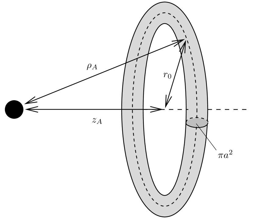
Figure 1: An atom near a dielectric ring (schematic picture).

From Fig. 1 we see that $|\mathbf{r}_{A}-\mathbf{s}|$ $\!\simeq$ $\!\sqrt{z_{A}^{2}+r_{0}^{2}}$ $\!\equiv$ $\!\rho_{A}$ for $a$ $\!\ll$ $\!r_{0}$, so an evaluation of the (trivial) volume integral in Eq. (2) results in the first-order CP potential

$$\Delta_{1}U_{A}(\rho_{A})$$

$$\quad=-\frac{\hbar V}{32\pi^{3}\varepsilon_{0}\rho_{A}^{6}}\int_{0}^{\infty}\mathrm{d}u\,\alpha_{A}(iu)\chi(iu)g_{2}(u\rho_{A}/c),$$ (63)

which is attractive, as expected. In the retarded limit [Eq. (22) with $r_{-}$ $\!=$ $\!\rho_{A}$] Eq. (4.1) reduces to

$$\Delta_{1}U_{A}(\rho_{A})=-\frac{23\hbar cV\alpha_{A}(0)\chi(0)}{64\pi^{3}\varepsilon_{0}\rho_{A}^{7}}$$ (64)

[cf. Eq. (24)], while in the nonretarded limit [Eq. (25) with $r_{+}$ $\!=$ $\!\rho_{A}$] one easily finds

$$\Delta_{1}U_{A}(\rho_{A})=-\frac{3\hbar V}{16\pi^{3}\varepsilon_{0}\rho_{A}^{6}}\int_{0}^{\infty}\mathrm{d}u\,\alpha_{A}(iu)\chi(iu)$$ (65)

[cf. Eq. (27)]. In both limiting cases the CP potential thus reduces to simple asymptotic power laws in $\rho_{A}$, where as usual the leading (inverse) power is increased by one when going from the nonretarded to the retarded limit.

The first (single point) second-order correction term $\Delta_{2}^{1}U_{A}(\rho_{A})$ can simply be obtained from Eqs. (4.1)–(65) by means of the replacement (30), while the calculation of the second (two-point) term $\Delta_{2}^{2}U_{A}(\rho_{A})$ is a lot more difficult due to the factor $|\mathbf{s}_{1}$ $\!-$ $\!\mathbf{s}_{2}|$. We find (see App. B)

$$\Delta_{2}^{2}U_{A}(\rho_{A})=\frac{(0.05\pm 0.02)\hbar cV\alpha_{A}(0)\chi^{2}(0)}{\pi^{3}\varepsilon_{0}\rho_{A}^{7}}$$ (66)

in the retarded limit and

$$\Delta_{2}^{2}U_{A}(\rho_{A})=\frac{(0.08\pm 0.03)\hbar V}{\pi^{3}\varepsilon_{0}\rho_{A}^{6}}\int_{0}^{\infty}\mathrm{d}u\,\alpha_{A}(iu)\chi^{2}(iu)$$ (67)

in the nonretarded limit. Recalling Eqs. (28) and (30), Eqs. (64) and (66) imply that up to quadratic order in $\chi$ we have

$$U_{A}(\rho_{A})=-\frac{23\hbar cV\alpha_{A}(0)\chi(0)}{64\pi^{3}\varepsilon_{0}\rho_{A}^{7}}\Big{[}1-(0.47\pm 0.05)\chi(0)\Big{]}$$ (68)

in the retarded limit, while Eqs. (65) and (67) show that in the nonretarded limit

$$U_{A}(\rho_{A})=-\frac{3\hbar V}{16\pi^{3}\varepsilon_{0}\rho_{A}^{6}}$$

$$\ \times\int_{0}^{\infty}\mathrm{d}u\,\alpha_{A}(iu)\chi(iu)\Big{[}1-(0.77\pm 0.17)\chi(iu)\Big{]}.$$ (69)

The uncertainty in the magnitude of the contribution quadratic in $\chi$ is due to the approximations made when calculating $\Delta^{2}_{2}U(\rho_{A})$ (cf. App. B). However, irrespective of these approximations, Eqs. (68) and (4.1) show that the leading non-additive correction $\Delta^{2}_{2}U_{A}(\rho_{A})$ to the linear result $\Delta_{1}U_{A}(\rho_{A})$ does not change the powers in the asymptotic retarded and nonretarded distance laws ($\rho_{A}^{-7}$ and $\rho_{A}^{-6}$, respectively), but merely modifies the constants of proportionality. A similar result has been found when studying a dielectric half space Buhmann05b .

4.2 Many-body decomposition

The explicit evaluation of multiple spatial integrals [being the main difficulty when evaluating $\Delta^{2}_{2}U(\vec{r}_{A})$] can in fact be avoided in many cases by an appropriate decomposition of the body of interest, as shall be demonstrated in the following. To that end, let us decompose the body described by $\chi(\vec{r},\omega)$ [recall Eq. (7)] into smaller bodies numbered by $n$, so that

$$\chi(\vec{r},\omega)=\sum_{n}\chi_{n}(\vec{r},\omega)1_{V_{n}}(\vec{r}),$$ (70)

where

$$1_{V_{n}}(\vec{r})=\left\{\begin{array}[]{l}1\mbox{ for }\vec{r}\in V_{n},\\[2.15277pt] 0\mbox{ for }\vec{r}\notin V_{n}.\end{array}\right.$$ (71)

Substituting Eqs. (70) and (71) into Eq. (2), and slightly rearranging the terms, we obtain

$$\Delta_{k}U_{A}(\vec{r}_{A})=\sum_{l=1}^{k}\Delta_{k}^{l}U_{A}(\vec{r}_{A}),$$ (72)

where

$$\Delta_{k}^{l}U_{A}(\vec{r}_{A})=\sum_{n_{1}<\ldots<n_{l}}\Delta_{k}^{l}U_{A}^{n_{1}\ldots n_{l}}(\vec{r}_{A})$$ (73)

with

$$\Delta_{k}^{l}U_{A}^{n_{1}\ldots n_{l}}(\vec{r}_{A})=\sum_{(m_{1},\ldots,m_{k})\in\mathcal{I}^{k}_{n_{1}\ldots n_{l}}}W_{A}^{m_{1}\ldots m_{k}}(\vec{r}_{A})$$ (74)

is the sum of all $l$-body contributions of order $k$ in $\chi$. In Eq. (74),

$$W_{A}^{m_{1}\ldots m_{k}}(\vec{r}_{A})=\frac{(-1)^{k}\hbar\mu_{0}}{2\pi c^{2k}}$$

$$\times\int_{0}^{\infty}\!\mathrm{d}u\,u^{2k+2}\alpha_{A}(iu)\Biggl{[}\prod_{j=1}^{k}\int_{V_{m_{j}}}\!\!\mathrm{d}^{3}s_{j}\,\chi_{m_{j}}(\vec{s}_{j},iu)\Biggr{]}$$

$$\times\mathrm{Tr}\bigl{[}\overline{\mathsf{G}}(\vec{r}_{A},\vec{s}_{1},iu)\cdot\overline{\mathsf{G}}(\vec{s}_{1},\vec{s}_{2},iu)\cdots\overline{\mathsf{G}}(\vec{s}_{k},\vec{r}_{A},iu)\bigr{]},$$ (75)

and the notation

$$\mathcal{I}^{k}_{n_{1}\ldots n_{l}}$$

$$=\Bigl{\{}(m_{1},\ldots,m_{k})\in\{n_{1},\ldots,n_{l}\}^{k}|\;\forall i\;\exists j:m_{j}=n_{i}\Bigr{\}}$$ (76)

is used.

In particular, to linear order in $\chi$ we have

$$\Delta_{1}U_{A}(\vec{r}_{A}) \,=\Delta_{1}^{1}U_{A}(\vec{r}_{A})=\sum_{n}\Delta_{1}^{1}U_{A}^{n}(\vec{r}_{A})$$

$$\,=\sum_{n}W_{A}^{n}(\vec{r}_{A}),$$ (77)

so the CP potential is additive in this order. For the term quadratic in $\chi$, Eqs. (72)–(74) together with Eq. (4.2) reduce to

$$\Delta_{2}U_{A}(\vec{r}_{A})=\Delta_{2}^{1}U_{A}(\vec{r}_{A})+\Delta_{2}^{2}U_{A}(\vec{r}_{A})$$

$$\quad=\sum_{n}\Delta_{2}^{1}U_{A}^{n}(\vec{r}_{A})+\sum_{m<n}\Delta_{2}^{2}U_{A}^{mn}(\vec{r}_{A})$$

$$\quad=\sum_{n}W_{A}^{nn}(\vec{r}_{A})+\sum_{m<n}\bigl{[}W_{A}^{mn}(\vec{r}_{A})+W_{A}^{nm}(\vec{r}_{A})\bigr{]}.$$ (78)

Obviously, the second term on the r.h.s. of Eq. (4.2) is the (overall) two-body contribution to the CP potential up to quadratic order in $\chi$. It can be regarded as being the leading correction to the additivity of the potential. Clearly, the expansion can in principle be extended to arbitrarily high orders in $\chi$, whereby $k$-body interactions first appear at $k$th order in $\chi$. In particular, Eqs. (4.2) and (4.2) generalize the result that up to linear order in $\chi$ the CP potential of an atom near a homogeneous semi-infinite dielectric half space can be written as an (infinite) sum of thin-layer potentials Buhmann05 , whereas the contribution quadratic in $\chi$ also contains two-layer terms leading to a breakdown of additivity Buhmann05b .

To illustrate the application of Eqs. (72)–(4.2) to the calculation of the CP potential of complex bodies via decomposition into simpler bodies, let us consider an atom at position $-z_{A}$ ($z_{A}$ $\!>$ $0$) near a semi-infinite half space filled with a stratified dielectric medium, i.e.

$$\varepsilon(\vec{r},\omega)=1+\chi(\omega)p(z),$$ (79)

where $p(z)$ is some profile function [$p(z)$ $\!\geq$ $\!0$ for $z$ $\!\geq$ $\!0$, $p(z)$ $\!=$ $\!0$ for $z$ $\!<$ $\!0$], which may be normalized such that $\max p(z)$ $\!=$ $\!1$. We decompose the half space into a set of thin slices of equal thickness $d$ such that

$$d\max\{p^{\prime}(z)|z>0\}\ll 1.$$ (80)

From Eq. (4.2) it follows that $\Delta_{1}^{1}U_{A}(z_{A})$ is given by the sum over the slices, which for $d$ $\!\ll$ $z_{A}$ contribute

$$\Delta_{1}^{1}U_{A}^{n}(z_{A})=-\frac{\hbar\mu_{0}d}{4\pi^{2}}\int_{0}^{\infty}\!\!\mathrm{d}u\,u^{2}\alpha_{A}(iu)\int_{0}^{\infty}\!\!\mathrm{d}q\,q$$

$$\times e^{-2b(z_{\mathrm{A}}+nd)}\biggl{[}\biggl{(}\frac{bc}{u}\biggr{)}^{\!\!2}-1+\frac{1}{2}\biggl{(}\frac{u}{bc}\biggr{)}^{\!\!2}\biggr{]}\chi(iu)p(nd),$$ (81)

where

$$b=\sqrt{\frac{u^{2}}{c^{2}}+q^{2}}$$ (82)

(cf. Eq. (71) in Ref. Buhmann05b ), so after turning the sum into an integral one obtains

$$\Delta_{1}^{1}U_{A}(z_{A})=-\frac{\hbar\mu_{0}}{4\pi^{2}}\int_{0}^{\infty}\!\!\mathrm{d}u\,u^{2}\alpha_{A}(iu)\chi(iu)$$

$$\quad\times\int_{0}^{\infty}\!\!\mathrm{d}q\,qe^{-2bz_{\mathrm{A}}}P(2b)\biggl{[}\biggl{(}\frac{bc}{u}\biggr{)}^{\!\!2}-1+\frac{1}{2}\biggl{(}\frac{u}{bc}\biggr{)}^{\!\!2}\biggr{]},$$ (83)

where

$$P(x)=\int_{0}^{\infty}\mathrm{d}z\,e^{-xz}p(z)$$ (84)

is the Laplace transform of the profile function $p(z)$. In a similar way, the results

$$\Delta_{2}^{1}U_{A}^{n}(z_{A})=\frac{\hbar\mu_{0}d}{4\pi^{2}}\!\int_{0}^{\infty}\!\!\mathrm{d}u\,u^{2}\alpha_{A}(iu)\!\int_{0}^{\infty}\!\!\mathrm{d}q\,q$$

$$\times e^{-2b(z_{\mathrm{A}}+nd)}\biggl{[}\frac{1}{2}\biggl{(}\frac{bc}{u}\biggr{)}^{\!\!2}-\frac{3}{4}+\frac{1}{4}\biggl{(}\frac{u}{bc}\biggr{)}^{\!\!2}\biggr{]}\chi^{2}(iu)p(nd)$$ (85)

(cf. Eq. (74) in Ref. Buhmann05b ) and

$$\Delta_{2}^{2}U_{A}^{mn}(z_{A})=\frac{\hbar\mu_{0}d^{2}}{2\pi^{2}}\!\int_{0}^{\infty}\!\!\mathrm{d}u\,u^{2}\alpha_{A}(iu)\!\int_{0}^{\infty}\!\!\mathrm{d}q\,qb$$

$$\quad\times e^{-2b(z_{\mathrm{A}}+nd)}\biggl{[}\frac{1}{2}-\frac{1}{2}\biggl{(}\frac{u}{bc}\biggr{)}^{\!\!2}+\frac{1}{4}\biggl{(}\frac{u}{bc}\biggr{)}^{\!\!4}\biggr{]}$$

$$\qquad\times\chi(iu)p(md)\chi(iu)p(nd)$$ (86)

(cf. Eq. (75) in Ref. Buhmann05b ) can be derived, leading to

$$\Delta_{2}^{1}U_{A}(z_{A})=\frac{\hbar\mu_{0}}{4\pi^{2}}\int_{0}^{\infty}\!\mathrm{d}u\,u^{2}\alpha_{A}(iu)\chi^{2}(iu)$$

$$\times\int_{0}^{\infty}\!\mathrm{d}q\,qe^{-2bz_{\mathrm{A}}}P(2b)\biggl{[}\frac{1}{2}\biggl{(}\frac{bc}{u}\biggr{)}^{\!\!2}-\frac{3}{4}+\frac{1}{4}\biggl{(}\frac{u}{bc}\biggr{)}^{\!\!2}\biggr{]}$$ (87)

and

$$\Delta_{2}^{2}U_{A}(z_{A})=\frac{\hbar\mu_{0}}{2\pi^{2}}\int_{0}^{\infty}\!\mathrm{d}u\,u^{2}\alpha_{A}(iu)\chi^{2}(iu)$$

$$\quad\times\int_{0}^{\infty}\!\mathrm{d}q\,qbe^{-2bz_{\mathrm{A}}}\biggl{[}\frac{1}{2}-\frac{1}{2}\biggl{(}\frac{u}{bc}\biggr{)}^{\!\!2}+\frac{1}{4}\biggl{(}\frac{u}{bc}\biggr{)}^{\!\!4}\biggr{]}$$

$$\qquad\quad\times\int_{0}^{\infty}\mathrm{d}z\,p(z)\int_{z}^{\infty}\mathrm{d}z^{\prime}\,e^{-2bz^{\prime}}p(z^{\prime}),$$ (88)

respectively. Hence the CP potential of the inhomogeneous half space up to quadratic order of $\chi$ has been calculated from the known CP potentials of one and two thin plates of constant permittivities. Needless to say that the method can be carried out to higher orders of $\chi$ and can also be applied to other than planar systems.

To give an example, we consider a dielectric medium whose permittivity oscillates in the $z$ direction,

$$\varepsilon(\vec{r},\omega)=1+\chi(\omega)\cos^{2}(k_{z}z)\Theta(z)$$ (89)

[$\Theta(z)$, unit step function]. Using Eqs. (4.2), (4.2), and (4.2), we find that up to quadratic order in $\chi$ the CP potential takes the asymptotic form (see App. C)

$$U_{A}(z_{A})=-\frac{1}{z_{A}^{4}}\Bigl{\{}\Delta_{1}C_{4}F_{3}(k_{z}z_{A})$$

$$\qquad+\Delta_{2}C_{4}\Bigl{[}{\textstyle\frac{126}{169}}F_{3}(k_{z}z_{A})+{\textstyle\frac{43}{169}}H_{3}(k_{z}z_{A})\Bigr{]}\Bigr{\}}$$ (90)

in the retarded limit [Eq. (22) with $r_{-}$ $\!=$ $z_{A}$] and

$$U_{A}(z_{A})=-\frac{(\Delta_{1}C_{3}+\Delta_{2}C_{3})F_{2}(k_{z}z_{A})}{z_{A}^{3}}$$ (91)

in the nonretarded limit [Eq. (25) with $r_{+}$ $\!=$ $z_{A}$]. Here,

$$\Delta_{1}C_{4}= \,\frac{23\hbar c\alpha_{A}(0)\chi(0)}{640\pi^{2}\varepsilon_{0}}\,,$$ (92)

$$\Delta_{2}C_{4}= \,-\frac{169\hbar c\alpha_{A}(0)\chi^{2}(0)}{8960\pi^{2}\varepsilon_{0}}\,,$$ (93)

$$\Delta_{1}C_{3}= \,\frac{\hbar}{32\pi^{2}\varepsilon_{0}}\int_{0}^{\infty}\mathrm{d}u\,\alpha_{A}(iu)\chi(iu)\,,$$ (94)

$$\Delta_{2}C_{3}= \,-\frac{\hbar}{64\pi^{2}\varepsilon_{0}}\int_{0}^{\infty}\mathrm{d}u\,\alpha_{A}(iu)\chi^{2}(iu)$$ (95)

are just the linear and and quadratic expansions of the well-known coefficients for the homogeneous half space in the retarded and nonretarded limits [where $U_{A}(z_{A})$ $\!=$ $\!-C_{4}/z_{A}^{4}$, and $U(z_{A})$ $\!=$ $\!-C_{3}/z_{A}^{3}$, respectively], and the structure functions

$$F_{j}(x)=\frac{2^{j}}{j!}\int_{0}^{\infty}\mathrm{d}t\,t^{j}e^{-2t}\,\frac{2t^{2}+x^{2}}{t^{2}+x^{2}}\,,$$ (96)

$$H_{j}(x)=\frac{2^{j}}{j!}\int_{0}^{\infty}\!\mathrm{d}t\,t^{j}e^{-2t}\,\frac{2t^{6}\!+\!8x^{2}t^{4}\!+\!5x^{4}t^{2}\!+\!2x^{6}}{(t^{2}\!+\!x^{2})^{2}(t^{2}\!+\!4x^{2})}$$ (97)

are normalized such that

$$F_{j}(x)\to\biggl{\{}\begin{array}[]{lcl}1&\mathrm{for}&x\to 0,\\ {\textstyle\frac{1}{2}}&\mathrm{for}&x\to\infty,\end{array}$$ (100)

$$H_{j}(x)\to\biggl{\{}\begin{array}[]{lcl}1&\mathrm{for}&x\to 0,\\ {\textstyle\frac{1}{4}}&\mathrm{for}&x\to\infty.\end{array}$$ (103)

Equations (4.2) and (91), respectively, are illustrated in Figs. 2 and 3.

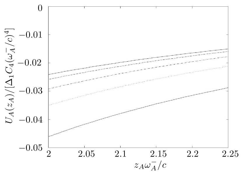
Figure 2: The CP potential of a ground-state atom in front of a half space with oscillating susceptibility in the retarded limit is displayed as a function of the distance $z_{A}$, where $k_{z}c/\omega_{A}^{-}$ $\!\to$ $\!\infty$ (upper solid line), $k_{z}c/\omega_{A}^{-}$ $\!=$ $\!4$ (dashed line), $k_{z}c/\omega_{A}^{-}$ $\!=$ $\!2$ (dash-dotted line), $k_{z}c/\omega_{A}^{-}$ $\!=$ $\!1$ (dotted line), $k_{z}c/\omega_{A}^{-}$ $\!\to$ $\!0$ (lower solid line), $\chi(0)$ $\!=$ $\!\frac{1}{2}$.

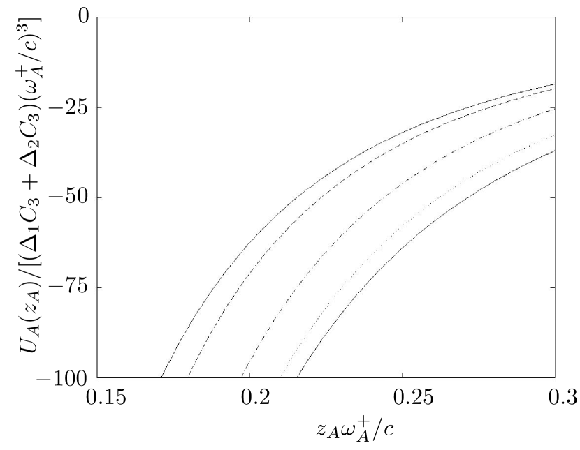
Figure 3: The CP potential of a ground-state atom in front of a half space with oscillating susceptibility in the non-retarded limit is displayed as a function of the distance $z_{A}$, where $k_{z}c/\omega_{A}^{+}$ $\!\to$ $\!\infty$ (upper solid line), $k_{z}c/\omega_{A}^{+}$ $\!=$ $\!20$ (dashed line), $k_{z}c/\omega_{A}^{+}$ $\!=$ $\!6$ (dash-dotted line), $k_{z}c/\omega_{A}^{+}$ $\!=$ $\!2$ (dotted line), $k_{z}c/\omega_{A}^{-}$ $\!\to$ $\!0$ (lower solid line).

It is seen that the potential curves for different values of $k_{z}$ lie between the two solid curves that correspond to the limiting cases $k_{z}$ $\!\to$ $\!\infty$ (upper curves) and $k_{z}$ $\!\to$ $\!0$ (lower curves, which represent the potential observed in the case of the respective homogeneous half space). From Eqs. (4.2), (91), and (100) it follows that the upper-curve potential values obtained in linear order of $\chi$ are $1/2$ times the lower-curve ones, which reflects the fact that for $k_{z}$ $\!\to$ $\!\infty$ the potential in linear order of $\chi$ is simply determined by the average permittivity $\varepsilon(\vec{r},\omega)$ $\!\simeq$ $\!1+\frac{1}{2}\chi(\omega)\Theta(z)$, cf. Eq. (89). The factor found for the quadratic-order term is equal to $1/2$ in the non-retarded limit [cf. Eqs. (91) and (100)], but equal to $295/676$ in the retarded limit [cf. Eqs. (4.2), (100), and (103)], owing to the influence of the two-plate term $\Delta_{2}^{2}U_{A}(z_{A})$. Note that the curves for the intermediate values of $k_{z}$ approach the upper limiting curve for large values of $z_{A}$ and the lower limiting curve for small values of $z_{A}$, the potentials thus being (near $z_{A}$ $\!\simeq$ $k_{z}^{-1}$) somewhat steeper than $z_{A}^{-4}$ and $z_{A}^{-3}$—the power laws observed in the case of a homogeneous half space. By controlling $k_{z}$, one can therefore control the shape of the potentials.

5 Summary

Within leading-order perturbation theory, the CP potential of a ground-state atom near dielectric bodies can be expressed in terms of the atomic polarizability and the scattering Green tensor of the body-assisted electromagnetic field, where the bodies are characterized by a spatially varying dielectric susceptibility that is a complex function of frequency. Starting from this very general formula, we have performed a Born expansion of the Green tensor to obtain an expansion of the CP potential in powers of the electric susceptibility. The expansion shows that only in linear order the CP force is a sum of attractive central forces, while higher-order terms are unavoidably connected to multiple-point correlations in the dielectric matter, leading to a breakdown of additivity.

Using the Born series, we have shown that when the dielectric bodies can be described by a susceptibility of Clausius-Mosotti type, i.e., when the basic constituents can be regarded as atom-like, then the CP potential is the (infinite) sum of all microscopic many-atom vdW potentials between the atom under consideration and the atoms forming the bodies. As a by-product, a general formula for the many-atom vdW potential of arbitrary order and on an arbitrary background of dielectric bodies has been found, which generalizes previous results found for atoms in vacuum.

Apart from being useful for making contact with microscopic descriptions of the CP force, the Born series can also be used for practical calculations, particularly when the Green tensor is not available in closed form. We have employed two strategies. (i) By direct evaluation of multiple spatial integrals, we have determined the attractive CP potential of a weakly dielectric ring, finding asymptotic $1/\rho_{A}^{7}$ and $1/\rho_{A}^{6}$ power laws in the retarded and the nonretarded limits, respectively. (ii) By reduction to simpler bodies with known CP potentials, we have derived expressions for the CP potential of an atom placed in front of an inhomogeneous stratified half space, with special emphasis on an oscillating susceptibility. In this case the potential exhibits—for distances comparable to the oscillation period—a somewhat stronger power law than in the case of a homogeneous half space.

Appendix A Derivation of the expansion in terms of many-atom vdW potentials [Eq. (3)]

As a preparation, we derive the symmetrization (3). The completely symmetrized form of a many-atom potential is given by

$$\mathcal{S}f(\vec{r}_{1},\ldots,\vec{r}_{j})\equiv\frac{1}{(2-\delta_{2j})j}\sum_{\pi\in P(j)}f(\vec{r}_{\pi(1)},\ldots,\vec{r}_{\pi(j)}),$$ (104)

where $P(j)$ denotes the permutation group of the numbers $1,\ldots,j$ and $1/(2-\delta_{2j})j$ is a normalization factor. As a trivial consequence of the cyclic property of the trace as well as the symmetry property of the Green tensor Knoll01

$$\mathsf{G}(\vec{r},\vec{r}^{\prime},\omega)=\mathsf{G}^{\top}(\vec{r}^{\prime},\vec{r},\omega)$$ (105)

together with Eq. (50) one easily finds that

$$\mathrm{Tr}\bigl{[}\overline{\mathsf{H}}(\vec{r}_{1},\vec{r}_{2},\omega)\cdots\overline{\mathsf{H}}(\vec{r}_{j},\vec{r}_{1},\omega)\bigr{]}$$

$$\quad=\mathrm{Tr}\bigl{[}\overline{\mathsf{H}}(\vec{r}_{\pi(1)},\vec{r}_{\pi(2)},\omega)\cdots\overline{\mathsf{H}}(\vec{r}_{\pi(j)},\vec{r}_{\pi(1)},\omega)\bigr{]}$$ (106)

if $\pi$ is either a cyclic permutation [e.g., $\pi(1)$ $\!=$ $\!2$, $\pi(2)$ $\!=$ $\!3$, $\ldots$ , $\pi(j)$ $\!=$ $\!1$] or the reverse of a cyclic permutation [e.g., $\pi(1)$ $\!=$ $\!j$, $\pi(2)$ $\!=$ $\!j-1$, $\ldots$ , $\pi(j)$ $\!=$ $\!1$]. With $f(\vec{r}_{1},\ldots,\vec{r}_{j})$ being given by the l.h.s. of Eq. (A), the sum on the r.h.s. of Eq. (104) contains classes of $(2-\delta_{2j})j$ terms that give the same result (note that for $j$ $\!=$ $\!2$ the cyclic permutation and its reverse coincide, so we have only $j$ instead of $2j$ terms in the class). By forming a set $\overline{P}(j)$ $\!\varsubsetneq$ $\!P(j)$ containing exactly one representative of each class (where obviously $\overline{P}(j)$ has $j!/$ $\![(2\!-\!\delta_{2j})j]$ members), the sum can thus be simplified, leading to Eq. (3).

With this preparation at hand, we may derive Eq. (3) [together with Eqs. (3) and (3)] by following these steps: We substitute Eqs. (47) and (50) into Eq. (2), multiply out and perform all spatial integrals over delta functions, where only terms of the form $\delta(\vec{s}_{j}-\vec{s}_{j+1})$ contribute [terms of the form $\delta(\vec{r}_{A}-\vec{s}_{j})$ giving zero integrals, because of $n(\vec{r}_{A})$ $\!=$ $\!0$, cf. the remark below Eq. (47)]. After renaming the remaining integration variables according to

$$\Biggl{[}\prod_{j=1}^{l}\int\mathrm{d}^{3}s_{j}\,n(\vec{s}_{j})\Biggr{]}f(\vec{s}_{1},\ldots,\vec{s}_{l})$$

$$=\frac{1}{l!}\sum_{\pi\in P(l)}\Biggl{[}\prod_{j=1}^{l}\int\mathrm{d}^{3}s_{j}\,n(\vec{s}_{j})\Biggr{]}f(\vec{s}_{\pi(1)},\ldots,\vec{s}_{\pi(l)}),$$ (107)

the result may be written in the form

$$\Delta_{k}U_{A}(\vec{r}_{A})=\sum_{l=1}^{k}\Delta_{k}^{l}U_{A}(\vec{r}_{A}),$$ (108)

with

$$\Delta_{k}^{l}U_{A}(\vec{r}_{A})= \,\frac{1}{l!}\int_{0}^{\infty}\mathrm{d}u\Biggl{[}\prod_{j=1}^{l}\int\frac{\mathrm{d}^{3}s_{j}\,n(\vec{s}_{j})}{1\!-\!\frac{1}{3}\varepsilon_{0}^{-1}n(\vec{s}_{j})\alpha_{B}(\omega)}\Biggr{]}$$

$$\times\!\!\!\sum_{\begin{array}[]{c}\scriptstyle\eta_{1}\geq 0,\ldots,\eta_{l}\geq 0\\ \scriptstyle\eta_{1}+\ldots+\eta_{l}=k-l\end{array}}q^{\eta_{1}}(\vec{s}_{1},iu)\cdots q^{\eta_{l}}(\vec{s}_{l},iu)$$ (111)

$$\times U_{AB\ldots B}(\vec{r}_{A},\vec{s}_{1},\ldots,\vec{s}_{l},iu),$$ (112)

where each power of the factor

$$q(\vec{r},\omega)=\frac{-\frac{1}{3}\varepsilon_{0}^{-1}n(\vec{r})\alpha_{B}(\omega)}{1-\frac{1}{3}\varepsilon_{0}^{-1}n(\vec{r})\alpha_{B}(\omega)}$$ (113)

is due to the integration of one term containing $\delta(\vec{s}_{j}-\vec{s}_{j+1})$, and

$$\int_{0}^{\infty}\mathrm{d}u\,U_{AB\ldots B}(\vec{r}_{1},\ldots,\vec{r}_{l+1},iu)$$

$$=U_{AB\ldots B}(\vec{r}_{1},\ldots,\vec{r}_{l+1}),$$ (114)

recall Eq. (3). Summing Eq. (108) over $k$, and rearranging the double sum, we find

$$\sum_{k=1}^{\infty}\Delta_{k}U_{A}(\vec{r}_{A})=\sum_{k=1}^{\infty}\sum_{l=1}^{k}\Delta_{k}^{l}U_{A}(\vec{r}_{A})=\sum_{l=1}^{\infty}\Delta^{l}U_{A}(\vec{r}_{A}),$$ (115)

where

$$\Delta^{l}U_{A}(\vec{r}_{A})=\frac{1}{l!}\int_{0}^{\infty}\!\!\mathrm{d}u\,\Biggl{[}\prod_{j=1}^{l}\int\mathrm{d}^{3}s_{j}\,$$

$$\quad\times\frac{n(\vec{s}_{j})}{1-\frac{1}{3}\varepsilon_{0}^{-1}n(\vec{s}_{j})\alpha_{B}(iu)}\sum_{\eta_{j}=0}^{\infty}q^{\eta_{j}}(\vec{s}_{j},iu)\Biggr{]}$$

$$\quad\times U_{AB\ldots B}(\vec{r}_{A},\vec{s}_{1},\ldots,\vec{s}_{l},iu).$$ (116)

After performing the geometric sums

$$\sum_{j=0}^{\infty}q^{j}(\vec{r},\omega)=1-{\textstyle\frac{1}{3}}\varepsilon_{0}^{-1}n(\vec{r})\alpha_{B}(\omega),$$ (117)

cf. Eq. (113), the denominators in Eq. (A) cancel, so by recalling Eqs. (11), (A) and (115), we arrive at Eq. (3) together with Eqs. (3) and (3).

Appendix B Calculation of the two-point correlation term for the dielectric ring [Eqs. (66) and (67)]

An approximation to the two-point correlation term in the retarded limit as given by Eq. (2)–(2) [together with Eqs. (33)–(35) and Eq. (37)] in the case of the dielectric ring can be obtained by replacing the variable $\vec{s}_{1}$ by its average across the cross section of the ring ($|\mathbf{r}_{A}-\mathbf{s}_{1}|$ $\!\simeq$ $\!\rho_{A}$ for $a$ $\!\ll$ $\!r_{0}$), evaluating the $\vec{s}_{1}$-integral, and separating the $\vec{s}_{2}$-integral into two parts,

$$\Delta_{2}^{2}U_{A}(\vec{r}_{A})=\frac{\hbar cV\alpha_{A}(0)\chi^{2}(0)}{32\pi^{4}\varepsilon_{0}}$$

$$\quad\times\Biggl{\{}\int_{-\lambda a}^{\lambda a}\mathrm{d}z\int_{0}^{a}\mathrm{d}\rho\,\rho\int_{0}^{2\pi}\mathrm{d}\phi+\pi a^{2}\int_{\lambda a/r_{0}}^{2\pi-\lambda a/r_{0}}r_{0}\mathrm{d}\theta\Biggr{\}}$$

$$\quad\times\frac{1}{\alpha^{3}\beta^{3}\gamma^{3}(\alpha\!+\!\beta\!+\!\gamma)}\bigl{[}f_{1}(\alpha,\beta,\gamma)+f_{2}(\gamma,\alpha,\beta)(\hat{\bm{\alpha}}\!\cdot\!\hat{\bm{\beta}})^{2}$$

$$\quad+f_{2}(\alpha,\beta,\gamma)(\hat{\bm{\beta}}\!\cdot\!\hat{\bm{\gamma}})^{2}+f_{2}(\beta,\gamma,\alpha)(\hat{\bm{\gamma}}\!\cdot\!\hat{\bm{\alpha}})^{2}$$

$$\quad+f_{3}(\alpha,\beta,\gamma)(\hat{\bm{\alpha}}\!\cdot\!\hat{\bm{\beta}})(\hat{\bm{\beta}}\!\cdot\!\hat{\bm{\gamma}})(\hat{\bm{\gamma}}\!\cdot\!\hat{\bm{\alpha}})\bigr{]}$$

$$\equiv\Delta_{2}^{2,\mathrm{c}}U_{A}(\vec{r}_{A})+\Delta_{2}^{2,\mathrm{r}}U_{A}(\vec{r}_{A})$$ (118)

where the integral in $\Delta_{2}^{2,\mathrm{c}}U_{A}(\vec{r}_{A})$ extends over an approximately cylindrical volume of cross section $\pi a^{2}$ and length $2\lambda a$, and that in $\Delta_{2}^{2,\mathrm{r}}U_{A}(\vec{r}_{A})$ extends over the volume of the remaining open ring.

For the integral in $\Delta_{2}^{2,\mathrm{c}}U_{A}(\vec{r}_{A})$, we may approximate

$$\qquad\alpha=\gamma\simeq\rho_{A},\quad\beta\simeq\sqrt{z^{2}+\rho^{2}},$$

$$\hat{\bm{\alpha}}\!\cdot\!\hat{\bm{\beta}}=-\hat{\bm{\beta}}\!\cdot\!\hat{\bm{\gamma}}\simeq\frac{\rho\cos(\phi)}{\sqrt{z^{2}+\rho^{2}}},\quad\hat{\bm{\gamma}}\!\cdot\!\hat{\bm{\alpha}}\simeq-1$$ (119)

for $a$ $\!\ll$ $\!r_{0}$, and Eqs. (2)–(2) [recall Eq. (37)] simplify to

$$f_{1}(\alpha,\beta,\gamma)\simeq\frac{13}{8},\quad f_{2}(\alpha,\beta,\gamma)=f_{2}(\gamma,\alpha,\beta)\simeq\frac{15}{8},$$

$$\qquad f_{2}(\beta,\gamma,\alpha)\simeq-\frac{3}{4},\quad f_{3}(\alpha,\beta,\gamma)\simeq-\frac{51}{8}.$$ (120)

Substituting Eqs. (B) and (B) into Eq. (B), carrying out the $\phi$-integral, and using

$$\int_{-\lambda a}^{\lambda a}\mathrm{d}z\int_{0}^{a}\mathrm{d}\rho\,\rho\frac{2z^{2}-\rho^{2}}{\sqrt{z^{2}+\rho^{2}}^{5}}=\frac{2\lambda}{\sqrt{1+\lambda^{2}}}\,,$$ (121)

one may find

$$\Delta_{2}^{2,\mathrm{c}}U_{A}(\vec{r}_{A})=\frac{7\hbar cV\alpha_{A}(0)\chi^{2}(0)}{256\pi^{3}\varepsilon_{0}\rho_{A}^{7}}\times\frac{\lambda}{\sqrt{1+\lambda^{2}}}.$$ (122)

For the integral in $\Delta_{2}^{2,\mathrm{r}}U_{A}(\vec{r}_{A})$, the approximations

$$\alpha=\gamma\simeq\rho_{A},\quad\beta\simeq 2r_{0}|\sin(\theta/2)|,$$

$$\hskip 8.61108pt\hat{\bm{\alpha}}\!\cdot\!\hat{\bm{\beta}}=\hat{\bm{\beta}}\!\cdot\!\hat{\bm{\gamma}}\simeq-\frac{r_{0}|\sin(\theta/2)|}{\rho_{A}},$$

$$\hskip 21.52771pt\hat{\bm{\gamma}}\!\cdot\!\hat{\bm{\alpha}}\simeq\frac{2r_{0}^{2}\sin^{2}(\theta/2)}{\rho_{A}^{2}}-1$$ (123)

are valid for $a$ $\!\ll$ $\!r_{0}$. Inspection of Eq. (B) shows that the leading term in $(a/r_{0})$ of $\Delta_{2}^{2,\mathrm{r}}U_{A}(\vec{r}_{A})$ is due to the factor $\beta^{3}$ $\!\propto$ $\sin^{3}(\theta/2)$ in the denominator of the integrand [cf. Eq. (125) below], and comes from regions where $\sin(\theta/2)$ $\!\ll$ $\!1$. Hence we may apply a Taylor expansion in powers of $\sin(\theta/2)$, retaining only

$$f_{1}(\alpha,\beta,\gamma)\simeq\frac{13}{8},\quad f_{2}(\beta,\gamma,\alpha)\simeq-\frac{3}{4}.$$ (124)

Substituting Eqs. (B) and (124) into Eq. (B), and performing the $\theta$-integral using

$$\int_{\lambda a/r_{0}}^{2\pi-\lambda a/r_{0}}\!\!\frac{\mathrm{d}\theta}{|\sin^{3}(\theta/2)|}=8\Bigl{(}\frac{r_{0}}{\lambda a}\Bigr{)}^{2}+o\bigl{[}\ln(\lambda a/r_{0})\bigr{]},$$ (125)

eventually leads to

$$\Delta_{2}^{2,\mathrm{r}}U_{A}(\vec{r}_{A})=\frac{7\hbar cV\alpha_{A}(0)\chi^{2}(0)}{512\pi^{3}\varepsilon_{0}\rho_{A}^{7}}\times\frac{1}{\lambda^{2}},$$ (126)

so that

$$\Delta_{2}^{2}U_{A}(\vec{r}_{A})=\frac{7\hbar cV\alpha_{A}(0)\chi^{2}(0)}{512\pi^{3}\varepsilon_{0}\rho_{A}^{7}}\times f(\lambda),$$ (127)

where

$$f(\lambda)=\frac{1}{\lambda^{2}}+\frac{2\lambda}{\sqrt{1+\lambda^{2}}}$$ (128)

[recall Eq. (122)]. Note that the approximations made for calculating $\Delta_{2}^{2,\mathrm{c}}U_{A}(\vec{r}_{A})$ break down for large $\lambda$ while those made for calculating $\Delta_{2}^{2,\mathrm{r}}U_{A}(\vec{r}_{A})$ break down for small $\lambda$. We put

$$f(\lambda) \mapsto {\textstyle\frac{1}{2}}\biggl{[}\max_{0.5\leq\lambda\leq 1.5}f(\lambda)+\min_{0.5\leq\lambda\leq 1.5}f(\lambda)\biggr{]}$$ (129)

$$\pm{\textstyle\frac{1}{2}}\biggl{[}\max_{0.5\leq\lambda\leq 1.5}f(\lambda)-\min_{0.5\leq\lambda\leq 1.5}f(\lambda)\biggr{]}$$

$$= 3.5\pm 1.4,$$

in Eq. (127), resulting in Eq. (66).

A similar procedure may be applied in the nonretarded limit, where Eq. (2) leads to

$$\Delta_{2}^{2}U_{A}(\vec{r}_{A})=\frac{3\hbar V}{128\pi^{4}\varepsilon_{0}}\int_{0}^{\infty}\mathrm{d}u\,\alpha_{A}(iu)\chi^{2}(iu)$$

$$\quad\times\Biggl{\{}\int_{-\lambda a}^{\lambda a}\mathrm{d}z\int_{0}^{a}\mathrm{d}\rho\,\rho\int_{0}^{2\pi}\mathrm{d}\phi+\pi a^{2}\int_{\lambda a/r_{0}}^{2\pi-\lambda a/r_{0}}r_{0}\mathrm{d}\theta\Biggr{\}}$$

$$\quad\times\frac{1-3(\hat{\bm{\alpha}}\!\cdot\!\hat{\bm{\beta}})(\hat{\bm{\beta}}\!\cdot\!\hat{\bm{\gamma}})(\hat{\bm{\gamma}}\!\cdot\!\hat{\bm{\alpha}})}{\alpha^{3}\beta^{3}\gamma^{3}}$$

$$\equiv\Delta_{2}^{2,\mathrm{c}}U_{A}(\vec{r}_{A})+\Delta_{2}^{2,\mathrm{r}}U_{A}(\vec{r}_{A}).$$ (130)

Use of Eqs. (B) and (121) leads to

$$\Delta_{2}^{2,\mathrm{c}}U_{A}(\rho_{A})= \,\frac{3\hbar V}{64\pi^{3}\varepsilon_{0}\rho_{A}^{6}}\int_{0}^{\infty}\mathrm{d}u\,\alpha_{A}(iu)\chi^{2}(iu)$$

$$\,\times\frac{\lambda}{\sqrt{1+\lambda^{2}}}\,,$$ (131)

while using Eq. (B), neglecting the term $(\hat{\bm{\alpha}}\cdot\hat{\bm{\beta}})(\hat{\bm{\beta}}\cdot\hat{\bm{\gamma}})(\hat{\bm{\gamma}}\cdot\hat{\bm{\alpha}})$, and recalling Eq. (125), results in

$$\Delta_{2}^{2,\mathrm{r}}U_{A}(\rho_{A})=\frac{3\hbar V}{128\pi^{3}\varepsilon_{0}\rho_{A}^{6}}\int_{0}^{\infty}\mathrm{d}u\,\alpha_{A}(iu)\chi^{2}(iu)\times\frac{1}{\lambda^{2}}\,.$$ (132)

Combining Eqs. (B) and (132) in accordance with Eq. (B), we obtain

$$\Delta_{2}^{2}U_{A}(\rho_{A})=\frac{3\hbar V}{128\pi^{3}\varepsilon_{0}\rho_{A}^{6}}\int_{0}^{\infty}\mathrm{d}u\,\alpha_{A}(iu)\chi^{2}(iu)\times f(\lambda)\,,$$ (133)

which, in combination with Eq. (129), implies Eq. (67).

Appendix C Asymptotic power laws in the case of a half space with oscillating susceptibility [Eqs. (4.2) and (91)]

As a preparing step, we derive the linear and quadratic expansions in $\chi$ of the coefficients

$$C_{4}= \,\frac{3\hbar c\alpha_{A}(0)}{64\pi^{2}\varepsilon_{0}}\int_{1}^{\infty}\mathrm{d}v\,\Biggl{\{}\frac{[\chi(0)+1]v-\sqrt{\chi(0)+v^{2}}}{[\chi(0)+1]v+\sqrt{\chi(0)+v^{2}}}$$

$$\,\times\!\biggl{(}\frac{2}{v^{2}}-\frac{1}{v^{4}}\biggr{)}-\frac{v-\sqrt{\chi(0)+v^{2}}}{v+\sqrt{\chi(0)+v^{2}}}\times\frac{1}{v^{4}}\Biggr{\}}$$

$$= \,\Delta_{1}C_{4}+\Delta_{2}C_{4}+\ldots$$ (134)

and

$$C_{3}= \,\frac{\hbar}{16\pi^{2}\varepsilon_{0}}\int_{0}^{\infty}\mathrm{d}u\ \alpha_{A}(iu)\frac{\chi(iu)}{\chi(iu)+2}$$

$$= \,\Delta_{1}C_{3}+\Delta_{2}C_{3}+\ldots\,,$$ (135)

that can be found for the retarded and nonretarded distance laws of the homogeneous half space Buhmann05 . Substituting

$$\frac{[\chi(0)+1]v-\sqrt{\chi(0)+v^{2}}}{[\chi(0)+1]v+\sqrt{\chi(0)+v^{2}}}$$

$$\quad=\biggl{[}\frac{1}{2}-\frac{1}{4v^{2}}\biggr{]}\chi(0)-\biggl{[}\frac{1}{4}-\frac{1}{8v^{2}}\biggr{]}\chi^{2}(0)+\ldots\,,$$ (136)

$$\frac{v-\sqrt{\chi(0)+v^{2}}}{v+\sqrt{\chi(0)+v^{2}}}=-\frac{1}{4v^{2}}\chi(0)+\frac{1}{8v^{4}}\chi^{2}(0)+\ldots$$ (137)

into Eq. (C) and carrying out the remaining $v$-integral, we arrive at Eqs. (92) and (93), while Eq. (C) implies Eqs. (94) and (95).

The spatial integrals in Eqs. (4.2) [recall Eq. (84)], (4.2) and (4.2) can be carried out explicitly for $p(z)$ $\!=$ $\!\cos^{2}(k_{z}z)$,

$$\int_{0}^{\infty}\mathrm{d}z\,e^{-2bz}\cos^{2}(k_{z}z)=\frac{2b^{2}+k_{z}^{2}}{4b(b^{2}+k_{z}^{2})}\,,$$ (138)

$$\int_{0}^{\infty}\mathrm{d}z\,\cos^{2}(k_{z}z)\int_{z}^{\infty}\mathrm{d}z^{\prime}\,e^{-2bz^{\prime}}\cos^{2}(k_{z}z^{\prime})$$

$$\quad=\frac{2b^{6}+8b^{4}k_{z}^{2}+5b^{2}k_{z}^{4}+2k_{z}^{6}}{8b^{2}(b^{2}+k_{z}^{2})^{2}(b^{2}+4k_{z}^{2})}\,,$$ (139)

resulting in

$$\Delta_{1}^{1}U_{A}(z_{A})=-\frac{\hbar\mu_{0}}{16\pi^{2}}\int_{0}^{\infty}\!\!\mathrm{d}u\,u^{2}\alpha_{A}(iu)\chi(iu)\int_{0}^{\infty}\!\!\mathrm{d}q\,\frac{q}{b}$$

$$\quad\times e^{-2bz_{\mathrm{A}}}\frac{2b^{2}+k_{z}^{2}}{b^{2}+k_{z}^{2}}\Biggl{[}\biggl{(}\frac{bc}{u}\biggr{)}^{\!\!2}-1+\frac{1}{2}\biggl{(}\frac{u}{bc}\biggr{)}^{\!\!2}\Biggr{]},$$ (140)

$$\Delta_{2}^{1}U_{A}(z_{A})=\frac{\hbar\mu_{0}}{16\pi^{2}}\!\int_{0}^{\infty}\!\!\mathrm{d}u\,u^{2}\alpha_{A}(iu)\chi^{2}(iu)\!\int_{0}^{\infty}\!\!\mathrm{d}q\,\frac{q}{b}$$

$$\quad\times e^{-2bz_{\mathrm{A}}}\frac{2b^{2}+k_{z}^{2}}{b^{2}+k_{z}^{2}}\Biggl{[}\frac{1}{2}\biggl{(}\frac{bc}{u}\biggr{)}^{\!\!2}-\frac{3}{4}+\frac{1}{4}\biggl{(}\frac{u}{bc}\biggr{)}^{\!\!2}\Biggr{]},$$ (141)

$$\Delta_{2}^{2}U_{A}(z_{A})=\frac{\hbar\mu_{0}}{16\pi^{2}}\!\int_{0}^{\infty}\!\!\mathrm{d}u\,u^{2}\alpha_{A}(iu)\chi^{2}(iu)\!\int_{0}^{\infty}\!\!\mathrm{d}q\,\frac{q}{b}$$

$$\quad\times e^{-2bz_{\mathrm{A}}}\frac{2b^{6}+8b^{4}k_{z}^{2}+5b^{2}k_{z}^{4}+2k_{z}^{6}}{(b^{2}+k_{z}^{2})^{2}(b^{2}+4k_{z}^{2})}$$

$$\quad\times\Biggl{[}\frac{1}{2}-\frac{1}{2}\biggl{(}\frac{u}{bc}\biggr{)}^{\!\!2}+\frac{1}{4}\biggl{(}\frac{u}{bc}\biggr{)}^{\!\!4}\Biggr{]}.$$ (142)

In analogy to the procedure outlined in Ref. Buhmann05 , the retarded limit may conveniently be treated by introducing the new integration variable $v$ $\!=$ $\!bc/u$, transforming integrals according to

$$\int_{0}^{\infty}\mathrm{d}u\,u^{2} \int_{0}^{\infty}\mathrm{d}q\,\frac{q}{b}\,e^{-2bz_{\mathrm{A}}}\ldots$$

$$\mapsto c^{3}\int_{1}^{\infty}\frac{\mathrm{d}v}{v^{4}}\int_{0}^{\infty}\mathrm{d}b\,b^{3}\,e^{-2bz_{\mathrm{A}}}\ldots\ ,$$ (143)

applying the approximation (23), and carrying out the $v$-integrals. Application of this procedure to Eqs. (C), (C), and (C) leads to

$$\Delta_{1}^{1}U_{A}(z_{A})=-\frac{23\hbar c\alpha_{A}(0)\chi(0)F_{3}(k_{z}z_{A})}{640\pi^{2}\varepsilon_{0}z_{A}^{4}}\,,$$ (144)

$$\Delta_{2}^{1}U_{A}(z_{A})=\frac{9\hbar c\alpha_{A}(0)\chi^{2}(0)F_{3}(k_{z}z_{A})}{640\pi^{2}\varepsilon_{0}z_{A}^{4}}\,,$$ (145)

$$\Delta_{2}^{2}U_{A}(z_{A})=\frac{43\hbar c\alpha_{A}(0)\chi^{2}(0)H_{3}(k_{z}z_{A})}{8960\pi^{2}\varepsilon_{0}z_{A}^{4}}\,,$$ (146)

where we have introduced the definitions (96) and (97). Combining Eqs. (144)–(146) in accordance with Eq. (4.2) and using Eqs. (92) and (93), we arrive at Eq. (4.2).

The asymptotic behavior of Eqs. (C)–(C) in the nonretarded limit may be obtained by transforming the integral according to

$$\int_{0}^{\infty}\mathrm{d}u \int_{0}^{\infty}\mathrm{d}q\,\frac{q}{b}\,e^{-2bz_{\mathrm{A}}}\ldots$$

$$\mapsto\int_{0}^{\infty}\mathrm{d}u\,\int_{0}^{\infty}\mathrm{d}b\,e^{-2bz_{\mathrm{A}}}\ldots\ ,$$ (147)

retaining only the leading power of $u/(bc)$, carrying out the $b$-integral and discarding higher-order terms in $uz_{\mathrm{A}}/c$ (cf. Ref. Buhmann05 ), resulting in

$$\Delta_{1}^{1}U_{A}(z_{A})=-\frac{\hbar F_{2}(k_{z}z_{A})}{32\pi^{2}\varepsilon_{0}z_{A}^{3}}\int_{0}^{\infty}\mathrm{d}u\,\alpha_{A}(iu)\chi(iu)\,,$$ (148)

$$\Delta_{2}^{1}U_{A}(z_{A})=\frac{\hbar F_{2}(k_{z}z_{A})}{64\pi^{2}\varepsilon_{0}z_{A}^{3}}\int_{0}^{\infty}\mathrm{d}u\,\alpha_{A}(iu)\chi^{2}(iu)\,,$$ (149)

$$\Delta_{2}^{2}U_{A}(z_{A})=\frac{\hbar\mu_{0}H_{0}(k_{z}z_{A})}{32\pi^{2}z_{A}}\int_{0}^{\infty}\mathrm{d}u\,u^{2}\alpha_{A}(iu)\chi^{2}(iu)\,,$$ (150)

recall Eqs. (96) and (97). Upon using Eq. (4.2), Eqs. (148) –(150) lead to Eq. (91), where we have neglected the term proportional to $z_{A}^{-1}$ in consistency with the nonretarded limit and used Eqs. (94) and (95).