Atom interferometry measurement of the electric polarizability of lithium

Abstract

Using an atom interferometer, we have measured the static electric polarizability of ⁷Li $\alpha=(24.33\pm 0.16)\times 10^{-30}$ m³ $=164.19\pm 1.08$ atomic units with a $0.66$% uncertainty. Our experiment, which is similar to an experiment done on sodium in 1995 by D. Pritchard and co-workers, consists in applying an electric field on one of the two interfering beams and measuring the resulting phase-shift. With respect to D. Pritchard’s experiment, we have made several improvements which are described in detail in this paper: the capacitor design is such that the electric field can be calculated analytically; the phase sensitivity of our interferometer is substantially better, near $16$ mrad/$\sqrt{\mbox{Hz}}$; finally our interferometer is species selective so that impurities present in our atomic beam (other alkali atoms or lithium dimers) do not perturb our measurement. The extreme sensitivity of atom interferometry is well illustrated by our experiment: our measurement amounts to measuring a slight increase $\Delta v$ of the atom velocity $v$ when it enters the electric field region and our present sensitivity is sufficient to detect a variation $\Delta v/v\approx 6\times 10^{-13}$.

I Introduction

The measurement of the electric polarizability $\alpha$ of an atom is a difficult experiment: this quantity cannot be measured by spectroscopy, which can access only to polarizability differences, and one should rely either on macroscopic quantity measurements such as the electric permittivity (or the index of refraction) or on electric deflection of an atomic beam. For a review on polarizability measurements, we refer the reader to the book by Kresin and Bonin bonin97 . For alkali atoms, all the accurate experiments were based on the deflection of an atomic beam by an inhomogeneous electric field and, in the case of lithium, the most accurate previous measurement was done in 1974 by Bederson and co-workers molof74 , with the following result $\alpha=(24.3\pm 0.5)\times 10^{-30}$ m³. However, in 2003, Amini and Gould, using an atomic fountain amini03 , have measured the polarizability of cesium atom with a $0.14$% relative uncertainty, which is presently the smallest uncertainty on the electric polarisability of an alkali atom.

Atom interferometry, which can measure any weak modification of the atom propagation, is perfectly adapted to measure the electric polarizability of an atom: this was demonstrated in 1995 by D. Pritchard and co-workers ekstrom95 with an experiment on sodium atom and they obtained a very high accuracy, with a statistical and systematic uncertainties both equal to $0.25$%. This experiment was and remains difficult because an electric field must be applied on only one of the two interfering beams: one must use a capacitor with a thin electrode, a septum, which can be inserted between the two atomic beams.

Using our lithium atom interferometer delhuille02a ; miffre05 , we have made an experiment very similar to the one of D. Pritchard ekstrom95 and we have measured the electric polarizability of lithium with a $0.66$% uncertainty, limited by the uncertainty on the mean atom velocity and not by the atom interferometric measurement itself miffre05a . In the present paper, we are going to describe in detail our experiment with emphasis on the improvements with respect to the experiments of D. Pritchard’s group ekstrom95 ; roberts04 : we have designed a capacitor with an analytically calculable electric field; we have obtained a considerably larger phase sensitivity, thanks to a large atomic flux and an excellent fringe visibility; finally our interferometer, which uses laser diffraction, is species selective: the contribution of any impurity (heavier alkali atoms, lithium dimers) to the signal can be neglected.

We may recall that several experiments using atom interferometers have exhibited a sensitivity to an applied electric field shimizu92 ; nowak98 ; nowak99 but these experiments were not aimed at an accurate measurement of the electric polarizability. Two other atom interferometry experiments rieger93 ; morinaga96 using an inelastic diffraction process, so that the two interfering beams are not in the same internal state, have measured the difference of polarizability between these two internal states. Finally, two experiments sangster93 ; sangster95 ; zeiske95 have measured the Aharonov-Casher phase aharonov84 : this phase, which results from the application of an electric field on an atom with an oriented magnetic moment, is proportional to the electric field.

This paper is organized as follows. We briefly recall the principle of the experiment in part II. We then describe our electric capacitor in part III and the experiment in part IV. The analysis of the experimental data is done in part V and we discuss the polarizability result in part VI. A conclusion and two appendices complete the paper.

II Principle of the measurement

If we apply an electric field $E$ on an atom, the energy of its ground state decreases by the polarizability term:

$$U=-2\pi\epsilon_{0}\alpha E^{2}$$ (1)

When an atom enters a region with a non vanishing electric field, its kinetic energy increases by $-U$ and its wave vector $k$ becomes $k+\Delta k$, with $\Delta k$ given by $\Delta k=2\pi\epsilon_{0}\alpha E^{2}m/(\hbar k)$. The resulting phase shift $\phi$ of the atomic wave is given by:

$$\phi=\frac{2\pi\epsilon_{0}\alpha}{\hbar v}\int E^{2}(z)dz$$ (2)

where we have introduced the atom velocity $v=\hbar k/m$ and taken into account the spatial dependence of the electric field along the atomic path following the $z$-axis. This phase shift is inversely proportional to the atom velocity and this dependence will be included in our analysis of the results.

The principle of the experiment, illustrated on figure 1, is to measure this phase shift by applying an electric field on one of the two interfering beams in an atom interferometer ekstrom95 . This is possible only if the two beams are spatially separated so that a septum can be inserted between the two beams. This requirement could be suppressed by using an electric field with a gradient as in reference roberts04 but it seems difficult to use this arrangement for a high accuracy measurement, because an accurate knowledge of the values of the field and of its gradient at the location of the atomic beams would be needed.

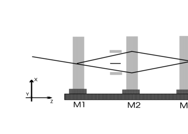
Figure 1: Schematic drawing of our experiment based on a Mach-Zehnder atom interferometer: a collimated atomic beam, coming from the left, is diffracted by three laser standing waves made by reflecting three laser beams on the mirrors $M_{1}$, $M_{2}$ and $M_{3}$. The output beam labelled $1$ is selected by a slit and detected by a hot-wire detector D. The capacitor with a septum between the two interfering beams is placed just before the second laser standing wave. The $x$, $y$ and $z$ axis are defined.

III The electric capacitor

III.1 Capacitor design

To make an accurate measurement, we must know precisely the electric field along the atomic path and guard electrodes are needed so that the length of the capacitor is well defined, as discussed by D. Pritchard and co-workers ekstrom95 . It would probably be better to have guard electrodes on both electrodes, but it seems very difficult to draw guard electrodes on the septum and to put them in place very accurately. Therefore, as in reference ekstrom95 , we have guard electrodes only on the massive electrodes. However, we have chosen to put our guard electrodes in the plane of the high voltage electrode. With this choice, the calculation of the electric field can be done analytically. Figure 2 presents two schematic drawings of the capacitor and defines our notations, while an artist’s view is presented in figure 3. Like in reference ekstrom95 , our capacitor is as symmetric as possible with respect to the septum plane, but, for a given experiment, only one half of the capacitor is used, the other part creating no electric field with $V=0$ everywhere.

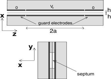
Figure 2: Two schematic drawings of the capacitor: top view of the capacitor cut in the atomic beam plane (upper panel) and end view as seen by an observer located on the atomic beam (lower panel). The axis being the same as in figure 1, the septum and the electrodes are parallel to the $y$, $z$ plane, with the septum at $x=0$ and the electrodes at $x=\pm h$. The high voltage electrodes at the $V=V_{0}$ potential extends from $z=-a$ to $z=+a$, while the guard electrodes extend outside with $|z|>a$. The septum and the guard electrodes are at the $V=0$ potential.

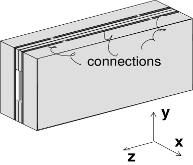
Figure 3: Artist’s view of the capacitor: we have also shown schematically some wires connecting the electrodes, the important point being that these wires are not close to the atomic beams.

III.2 Calculation of the capacitor electric field

III.2.1 From three dimensions to two dimensions

If a dielectric slab with a permittivity $\epsilon_{r}>1$ is introduced in a plane capacitor, the field lines are distorted and concentrated towards the slab. Because our capacitor contains dielectric spacers, one could fear a similar effect but this effect does not exist when the dielectric slab fills completely the gap between the electrodes. Following figure 2, the spacers, with a dielectric constant $\varepsilon_{r}$ completely fill the space $\left|y\right|>y_{0}$, with vacuum in the rest of capacitor, $\left|y\right|<y_{0}$. Let $V$ (respectively $V_{1}$) be the potential with $\left|y\right|<y_{0}$ ($\left|y\right|>y_{0}$). In the $\left|y\right|=y_{0}$ planes, the continuity equations give:

$$V=V_{1}{\mbox{ and }}\frac{\partial V}{\partial y}=\frac{\partial V_{1}}{\partial y}$$ (3)

As shown below, a 2D solution of the Laplace equation of the form $V(x,z)$ exists for the capacitor. Then clearly, if we take $V_{1}=V$, this solution fulfills both continuity equations on the dielectric borders in the $\left|y\right|=y_{0}$ planes and we know that the solution is unique.

III.2.2 Calculation of the potential and of the electric field

We consider only one half (with $x\geq 0$) of the capacitor represented on figure 2. We know the potential on the borders of the capacitor, with $V(x=0,z)=0$ and $V(x=h,z)=V_{0}$ if $\left|z\right|<a$ and $V(x=h,z)=0$ if $\left|z\right|>a$. To get the potential everywhere, we start by calculating the Fourier transform $\tilde{V}(k)$ of $V(x=h,z)$ :

$$\tilde{V}(k)=\frac{1}{\sqrt{2\pi}}\int_{-\infty}^{+\infty}V(x=h,z)\exp\left(-ikz\right)dz$$ (4)

Then, for a separable harmonic function of $x$ and $z$, with a $z$-dependence of the $\exp\left(ikz\right)$ form, its $x$-dependence is necessarily given by a linear combination of the two functions $\exp\left(\pm kx\right)$. Using this result and the conditions on the borders at $x=0$ and at $x=h$, we get the value of $V(x,z)$ everywhere:

$$V(x,z)=\frac{1}{\sqrt{2\pi}}\int_{-\infty}^{+\infty}\tilde{V}(k)\frac{\sinh\left(kx\right)}{\sinh\left(kh\right)}\exp\left(ikz\right)dk$$ (5)

from which we can deduce the electric field everywhere. On the septum surface $x=0$, the electric field is parallel to the $x$-axis and we can calculate exactly the integral of $E^{2}$ on this surface (see appendix A). We need the capacitor effective length $L_{eff}$ which is defined by:

$$L_{eff}=\frac{1}{E_{0}^{2}}\int_{-\infty}^{+\infty}E^{2}dz$$ (6)

where $E_{0}=V_{0}/h$ is the electric field of an infinite plane capacitor with the same electrode spacing $h$. Using equation (28), we get the exact value of $L_{eff}$:

$$L_{eff}=2a\left[\coth\left(\frac{\pi a}{h}\right)-\frac{h}{\pi a}\right]\approx 2a-\frac{2h}{\pi}$$ (7)

where exponentially small corrections of the order of $\exp\left[-2\pi a/h\right]$ have been neglected in the approximate result.

However, the atoms do not sample the electric field on the septum surface but at a small distance, of the order of $50$ $\mu$m in our experiment, and what we need is the integral of $E^{2}$ along their mean trajectory. This mean trajectory is not exactly parallel to the septum, but it is easier to calculate the integral along a constant $x$ line. We may use either the potential given by equation (5) or Maxwell’s equations to relate the field components near the septum surface to its value on the surface. The calculation, given in appendix A, proves that the first correction to the effective length is proportional to $x^{2}$:

$$L_{eff}\approx 2a-\frac{2h}{\pi}+\frac{2\pi x^{2}}{3h}$$ (8)

The $x^{2}$ correction is a fraction of the main term $2a$ equal to $\pi x^{2}/(3ah)$ and with our dimensions ($x\approx 50$ $\mu$m, $h\approx 2$ mm and $a\approx 25$ mm), this correction is close to $5\times 10^{-5}L_{eff}$. This correction is negligible at the present level of accuracy and we will use the value of $L_{eff}$ given by the approximate form of equation (7). More precisely, we will write:

$$\int_{-\infty}^{+\infty}E^{2}dz=V_{0}^{2}\left[\frac{2a}{h^{2}}-\frac{2}{\pi h}\right]$$ (9)

III.3 Construction of the capacitor

Let us describe how we build this capacitor. The external electrodes are made of glass plates ($80$ mm long in the $z$ direction, $35$ mm high in the $y$ direction, $10$ mm thick in the $x$ direction) covered by an evaporated aluminium layer. To separate the guard electrodes from the high voltage electrode, a gap is made in the aluminium layer by laser evaporation cheval . We found that $100$ $\mu$m wide gaps give a sufficient insulation under vacuum to operate the capacitor up to $V_{0}=500$ V. These gaps are separated by a distance $2a=50$ mm, so that the two guard electrodes are $15$ mm long. The glass spacers are $\sim 2$ mm thick plates of float glass ($10$ mm $\times$ $80$ mm) used without further polishing. The distance $y_{0}$ from the spacer inner edge to the atomic beam axis is equal to $\sim 7$ mm.

We have found that a float glass plate is flat within $\pm 2$ $\mu$m over the needed surface. This accuracy appeared to be sufficient for a first construction, as the main geometrical defects are due to the way we assemble the various parts by gluing them together and by an imperfect stretching of the septum. We use a double-faced tape ARCLAD 7418 (from Adhesive Research) to assemble the spacers on the external electrodes.

The septum is made of $6$ $\mu$m thick mylar from Goodfellow covered with aluminium on both faces. In a first step, the mylar sheet is glued on circular metal support. It is then covered by a thin layer of dish soap diluted in water and the mylar is heated near $80^{\circ}$C with a hot air gun. Then, we clean the mylar surface with water and let it dry. After this operation, the mylar is well stretched and its surface is very flat. We have measured the resonance frequencies of the drum thus formed, from which we deduced a surface tension of the order of $50$ N/m (this value is only indicative as this experiment was made with another mylar film which was $20$ $\mu$m thick). Once stretched, the mylar film is glued on one electrode-spacer assembly with an epoxy glue EPOTEK 301 (from Epoxy Technology), chosen for its very low viscosity, and then it is cut with a scalpel. In a final step, a second electrode-spacer assembly is glued on the other face of the mylar. Finally, as shown in figure 3, wires are connected to the various electrodes using an electrically conductive adhesive EPOTEK EE129-4 (also from Epoxy Technology).

III.4 Residual defects of the capacitor

We are going to discuss the various points by which the real capacitor differs from our model.

III.4.1 2D character of the potential

We have shown that the potential $V$ is reduced to a 2D function when an homogeneous dielectric slab fills completely the gap between the electrodes, with the border between the vacuum and the slab being a plane perpendicular to the electrodes. The real dielectric slab is the superposition of a tape, a glass spacer and a glue film, each material having a different permittivity $\epsilon_{r}$. The differences in permittivity perturb the potential which should take a 3D character extending on a distance comparable to the tape or glue film thicknesses. This perturbation seems negligible, because the tape and the glue films are very thin and also because these three dielectric materials have not very large $\epsilon_{r}$ values.

III.4.2 Do we know the potential everywhere on the border?

Our calculation assumes that the potential is known everywhere on the border. But, on the high-voltage electrode, we may fear that the potential is not well defined in the $100$ $\mu$m wide dielectric gaps separating the high voltage and guard electrodes as these gaps might get charged in an uncontrolled way. This is not likely if the volume resistivity $\rho$ of the pyrex glass used is not too large: more precisely, the time constant for the charge equilibration on the gap surface is given by $\epsilon_{0}\rho$ (within numerical factors of the order of one) and this time constant remains below $1$ second if $\rho\leq 10^{11}$ $\Omega$.m. We have found several values of the resistivity of pyrex glass at ordinary temperature, in the range $(4-8)\times 10^{8}$ $\Omega$.m and with such a conductivity, this time constant is below $10^{-2}$ s. Our calculation neglects the surface conductivity, due to the adsorbed impurities, which should further reduce this time constant.

Therefore, we think that it is an excellent approximation to assume that the potential $V$ makes a smooth transition from $V=0$ to $V=V_{0}$ in the gaps. Then, using equation (26), it is clear that the detailed shape of the transition has no consequence as these details are smoothed out by the convolution of $V(z)$ by the function $g(z)$ which has a full width at half maximum equal to $1.12h$. We can use equation (7) to calculate the effective length, provided that we add to the length of the high voltage electrode the mean width of the two gaps. In the present work, we have taken one gap width, $100$ $\mu$m, as a conservative error bar on the effective length. A superiority of our capacitor design is that these gaps are very narrow, thus minimizing the corresponding uncertainty on the capacitor effective length and we hope to be able to further reduce this uncertainty.

III.4.3 Parallelism of the electrodes

The thickness $h$ of the capacitor, which is the sum of the thickness of the spacers, the tape and the glue film, is not perfectly constant. Using a Mitutoyo Litematic machine, we have measured, with a $\pm 1$ $\mu$m uncertainty, the capacitor thickness as a function of $z$, in the center line of the two spacers, at $y=\pm 12$ mm. The average of these two measurements gives the thickness $h(z)$ in the $y=0$ plane around which the atom sample the electric field. The thickness $h$ is not perfectly constant but it is well represented by a linear function of $z$, given by $h(z)=h_{0}+h_{1}(z/a)$, the maximum deviation $h_{1}$ being considerably smaller than the mean $h$ value noted $h_{0}$. As these deviations are very small (see below), it seems reasonable to use use equation (9) provided that terms involving powers of $h$ are replaced by their correct averages. The first term in $h^{-2}$ corresponds to the integral of $E^{2}$ over the capacitor length, from $z=-a$ to $z=a$ and we must take the average value of $h^{-2}$ over this region. Neglecting higher order terms, this average is given by:

$$\left<\frac{1}{h^{2}}\right>=\frac{1}{h_{0}^{2}}\left[1+\frac{h_{1}^{2}}{h_{0}^{2}}\right]$$ (10)

In equation (9), the second term in $h^{-1}$, corresponds to end effects and this quantity must be replaced by the following two-point average:

$$\left<\frac{1}{h}\right>=\frac{1}{2}\left(\frac{1}{h(z=-a)}+\frac{1}{h(z=a)}\right)=\frac{1}{h_{0}}\left[1+\frac{h_{1}^{2}}{h_{0}^{2}}\right]$$ (11)

Both corrections involve the same factor $[1+(h_{1}^{2}/h_{0}^{2})]$.

III.4.4 Summary of the capacitor dimensions

Although the capacitor is as symmetric as possible, this symmetry is only approximate and we give the parameters for the half we have used for the set of measurements described below. The length of the high voltage electrode, including one gap width is $2a=50.00\pm 0.10$ mm, the error bar being taken equal to one gap width, as discussed above. The distance $h$ between the electrodes gap width is described by $h_{0}=2.056\pm 0.003$ mm and $h_{1}=3.2\times 10^{-3}$ mm. The correction term $h_{1}^{2}/h_{0}^{2}=2.4\times 10^{-6}$ is completely negligible.

IV The experiment

In this part, we are going to recall the main features of our lithium atom interferometer, to give the values of various parameters used for the present study, to present the data acquisition procedure and the way we extract the phases from the data.

IV.1 Our interferometer

Our atom interferometer is a Mach-Zehnder interferometer using Bragg diffraction on laser standing waves. Its design is inspired by the sodium interferometer of D. Pritchard and co-workers keith91 ; schmiedmayer97 and by the metastable neon interferometer of Siu Au Lee and co-workers giltner95b . A complete description has been published delhuille02a ; miffre05 .

The lithium atomic beam is a supersonic beam seeded in argon and, for the present experiment, we have worked with a low argon pressure in the oven $p_{0}=167$ mbar, because the detected lithium signal increases when the argon pressure decreases. The oven body temperature is equal to $973$ K, fixing the vapor pressure of lithium at $p_{Li}=0.8$ mbar and the nozzle temperature is equal to $T_{0}=1073$ K. With these source conditions, following our detailed analysis miffre05b , the argon and lithium velocity distributions are described by a parallel speed ratio for argon equal to $S_{\|,Ar}=8.3$ and a parallel speed ratio for lithium equal to $S_{\|,Li}=6.2$ (the parallel speed ratio is defined by equation (15) below).

We use Bragg diffraction on laser standing waves at $\lambda=671$ nm: the laser is detuned by about $3$ GHz on the blue side of the ${}^{2}S_{1/2}$ - ${}^{2}P_{3/2}$ transition of the ⁷Li isotope, the signal is almost purely due to this isotope, which has a natural abundance equal to $92.41$%, and not to the other isotope ${}^{6}Li$. Moreover, any other species present in the beam, for instance heavier alkali atoms or lithium dimers, is not diffracted and does not contribute to the signal.

The case of lithium dimers deserves a special discussion because they are surely present in the beam and the lithium dimer has an absorption band system due its $A-X$ transition with many lines around $671$ nm: for most rovibrational levels of the $X$ state, the absorption transition which is closest to the laser frequency has a very large detuning of the order of hundreds to thousands of GHz and the intensity of this resonance transition is also weaker than the resonance transition of lithium atom, because of the Franck-Condon factor. Therefore, the lithium dimers have a negligible probability of diffraction and do not contribute to the interferometer signals.

The interference signals in a Mach-Zehnder interferometer are given by:

$$I=I_{0}\left[1+{\mathcal{V}}\cos\psi\right]$$ (12)

where the phase $\psi$ of the interference fringes can be written:

$$\psi=p(2k_{L})(x_{1}+x_{3}-2x_{2})+\phi$$ (13)

The first term of $\psi$ is particular to three-grating interferometers: the diffracted beam of order $p$ by grating $i$ has a phase dependent on the grating position $x_{i}$. In our case of laser diffraction, the grating position $x_{i}$ is given by the mirror position $M_{i}$ and $2k_{L}$ is the grating wavevector, where $k_{L}$ is the laser wavevector. This phase term is very interesting because it is non dispersive and it is commonly used to observe interference fringes. In our case, we scan the position $x_{3}$ of mirror $M_{3}$ by a piezoelectric translation stage. The second term $\phi$ represent any phase difference between the two beams and in particular, it will represent the phase shift due to the application of an electric field on one of the two paths.

IV.2 Introduction of the capacitor

In the present work, we have only used the diffraction order $p=1$ so that the center of the two beams are separated by about $90$ $\mu$m at the location of the capacitor, which is located just before the second laser standing wave. The capacitor is attached to the top of the vacuum chamber and not to the rail supporting the laser standing wave mirrors $M_{i}$: in this way, we do not increase the vibrations of the mirror positions $x_{i}$ The capacitor is held by a translation stage along the $x$-direction, which can be adjusted manually thanks to a vacuum feedthrough and a double stage kinematic mount built in our laboratory. The first stage, operated with screws, can be used only when the experiment is at atmospheric pressure while the second stage, actuated by low-voltage piezo-translators, can be adjusted under vacuum. When the septum is inserted between the two atomic paths, the atom propagation is almost not affected by its presence and, as shown in figure 4, we have observed a fringe visibility equal $\mathcal{V}=84\pm 1$ % and a negligible reduction of the atomic flux.

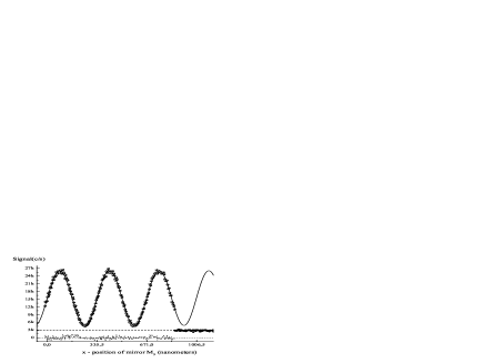
Figure 4: Interference signal observed by displacing the mirror $M_{3}$: the signal is expressed in counts per second, but the counting time is equal to $0.1$ second only and the background signal has been recorded at the end of the experiment. The full curve is the best fit and the fit residuals are plotted, at the bottom of the figure.

To optimize the phase sensitivity (see a discussion in reference miffre05 ), we have opened the collimation slit $S_{1}$ and the detection slit $S_{D}$ (see reference miffre05 ) with widths $e_{1}=18$ $\mu$m and $e_{D}=50$ $\mu$m, thus increasing the mean flux up to $10^{5}$ counts/s and slightly reducing the fringe visibility down to ${\mathcal{V}_{0}}=62$% (see figure 5).

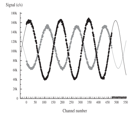
Figure 5: Experimental signals corresponding to $V_{0}=0$ (black dots) and to $V_{0}\approx 260$ Volts (grey dots). Their sinusoidal fits using equation (IV.4) are represented by the full curves. The phase shift due to the polarizability effect is close to $3\pi$ and the fringe visibility is reduced because of the dispersion of the phase shift associated to the velocity spread of the lithium atoms.

IV.3 The data acquisition procedure

We have made a series of recordings, labelled by an index $i$ from $1$ to $44$, with $V_{0}=0$ when $i$ is odd, and with $V_{0}\neq 0$, when $i$ is even with $V_{0}\approx 10\times i$ Volts. For each recording, we apply the same linear ramp on the piezo-drive of mirror $M_{3}$ in order to observe interference fringes and $471$ data points are recorded with a counting time per channel equal to $0.36$ s. Figure 5 presents a pair of consecutive recordings.

The high voltage power supply has stability close to $10^{-4}$ and the applied voltage is measured by a HP model $34401A$ voltmeter with a relative accuracy better than $10^{-5}$.

IV.4 Extracting phases from the data

For each recording, the data points $I_{i}(n)$ have been fitted by a function:

$$I_{i}(n) = I_{0i}\left[1+{\mathcal{V}}_{i}\cos\psi_{i}(n)\right]$$

$$\mbox{with }\psi_{i}(n) = a_{i}+b_{i}n+c_{i}n^{2}$$ (14)

where $n$ labels the channel number, $a_{i}$ represents the initial phase of the pattern, $b_{i}$ an ideal linear ramp and $c_{i}$ the non-linearity of the piezo-drive. For the $V_{0}=0$ recordings, $a_{i}$, $b_{i}$ and $c_{i}$ have been adjusted as well as the mean intensity $I_{0i}$ and the visibility ${\mathcal{V}}_{i}$. For the $V\neq 0$ recording, we have fitted only $a_{i}$, $I_{0i}$ and ${\mathcal{V}}_{i}$, while fixing $b_{i}$ and $c_{i}$ to their value $b_{i-1}$ and $c_{i-1}$ from the previous $V=0$ recording. We think that our best phase measurements are given by the mean phase $\bar{\psi}_{i}$ obtained by averaging $\psi_{i}(n)$ over the $471$ channels. The $1\sigma$ error bar of these mean phases are of the order of $2-3$ mrad, increasing with the applied voltage up to $23$ mrad because the visibility is considerably lower when the applied voltage $V_{0}$ is large (see figure 6). This rapid decrease of the visibility is due to the velocity dependence of the phase and to the velocity distribution of the lithium atoms.

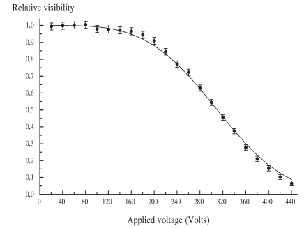
Figure 6: Relative fringe visibility ${\mathcal{V}}/{\mathcal{V}}_{0}$ with ${\mathcal{V}}_{0}=62$% as a function of the applied voltage $V_{0}$. The points are our measurements and the full curve is our best fit using equations (15,16).

The mean phase values $\bar{\psi}_{i}$ values of the $V_{0}=0$ recordings are plotted in figure 7: they present a drift equal to $7.5\pm 0.2$ mrad/minute and some scatter around this regular drift. The most natural explanation for this drift is a change of the phase $\psi$ resulting from a variation of the mirror positions $x_{i}$: $\psi$ changes by $1$ radian for a variation of $(x_{1}+x_{3}-2x_{2})$ equal to $53$ nm. We have verified that the observed drift has the right order of magnitude to be due to the differential thermal expansion of the structure supporting the three mirrors: its temperature was steadily drifting at $1.17\times 10^{-3}$ K/minute during the experiment and the support of mirror $M_{3}$ differs from the other supports, as it includes a piezo translation stage, which is replaced by aluminium alloy for the mirrors $M_{1}$ and $M_{2}$. Presently, we have no explanation of the phase scatter, which presents a quasi-periodic structure as a function of time: its rms value is equal to $33$ milliradian and, unfortunately, this scatter gives the dominant contribution to our phase uncertainty.

Figure 7: The mean phase value $\left<\psi_{i}\right>$, in radian, of the $V_{0}=0$ recordings is plotted as a function of the recording starting time $t$ in minutes (with an arbitrary origin). The straight line is the best linear fit, corresponding to a phase drift of $7.5\pm 0.2$ mrad/minute. The fit residuals are also plotted and from $t=15$ till $t=100$ minutes, the residuals exhibit an oscillating pattern with a period close to $17$ minutes.

The phase shift $\left<\phi(V_{0})\right>$ due to the polarizability effect (the average $\left<\right>$ recalls that our experiment makes an average over the velocity distribution, as discussed below) is taken equal to $\left<\phi(V_{0})\right>=\bar{\psi}_{i}-\left(\bar{\psi}_{i-1}+\bar{\psi}_{i+1}\right)/2$ where the recording $i$ corresponds to the applied voltage $V_{0}$: the average of the mean phase of the two $V_{0}=0$ recordings done just before and after is our best estimator of the mean phase of the interference signal in zero field. In figure 8, we have plotted the phase shift $\phi(V_{0})$ as a function of the applied voltage $V_{0}$. We have chosen for the error bar on $\phi(V_{0})$ the quadratic sum of the $1\sigma$ error bar given by the fit of $\left<\psi_{i}\right>$ and the $33$ milliradians rms deviation of the $V_{0}=0$ phase measurements.

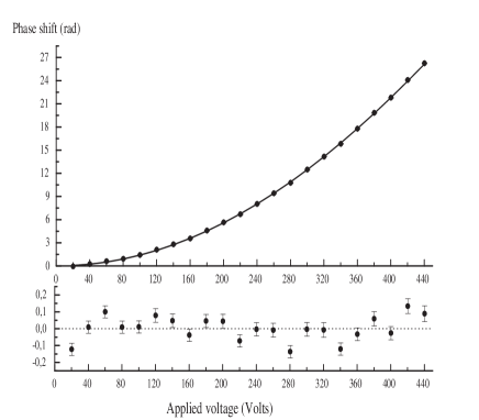
Figure 8: The measured phase shift $\left<\phi(V_{0})\right>$ in radian is plotted as a function of the applied voltage $V_{0}$: the best fit using equations (4,5) is represented by the full curve and the residuals are plotted in the lower graph with an expanded scale.

V Analysis of the signals: the effect of the lithium velocity distribution

To interpret the experimental data, we must take into account the velocity distribution of the lithium atoms.

V.1 Velocity averaging of the interference signal

We assume that this velocity distribution is given by:

$$P(v)=\frac{S_{\|}}{u\sqrt{\pi}}\exp\left[-\left((v-u)S_{\|}/u\right)^{2}\right]$$ (15)

where $u$ is the most probable velocity and $S_{\|}$ is the parallel speed ratio. With respect to the usual form of the velocity distribution for supersonic beams, we have omitted a $v^{3}$ factor which is traditionally introduced haberland85 but when the parallel speed ratio $S_{\|}$ is large enough, this $v^{3}$ has little effect and the main consequence of its omission is a slight modification of the values of $u$ and $S_{\|}$. Here, what we consider is the atoms contributing to the interferometer signal and their velocity distribution may differ slightly from the velocity of the incident beam, as Bragg diffraction is velocity selective. The experimental signal can be written:

$$I = I_{0}\int dvP(v)\left[1+{\mathcal{V}}_{0}\cos\left(\psi+\phi_{m}\frac{u}{v}\right)\right]$$ (16)

$$= I_{0}\left[1+\left<{\mathcal{V}}\right>\cos\left(\psi+\left<\phi\right>\right)\right]$$

where $\phi_{m}$ is the value of the phase $\phi$ for the velocity $v=u$. If we introduce $\delta=(v-u)/u$ and expand $(u/v)$ in powers of $\delta$ up to second order, the integral can be taken exactly, as discussed in appendix B. However, the accuracy of this approximation is not good enough when $\phi_{m}$ is large and we have used direct numerical integration to fit our data.

V.2 Numerical fit of the data

Using equations (15) and (16), we have fitted the measured phase $\phi$ and visibility ${\mathcal{V}}$ as a function of the applied voltage $V$. The phase measurements received a weight inversely proportional to the square of their estimated uncertainty and we have adjusted two parameters, the value of $\phi_{m}/V^{2}$ and the parallel speed ratio $S_{\|}$. The results of the fits are presented in figures 8 and 6. The agreement is excellent, in particular for the phase data, and we deduce a very accurate value of $\phi_{m}/V_{0}^{2}$:

$$\phi_{m}/V_{0}^{2}=(1.3870\pm 0.0010)\times 10^{-4}\mbox{ rad/V}^{2}$$ (17)

where the error bar is equal to $1\sigma$. The relative uncertainty on $\phi_{m}/V_{0}^{2}$ is very small, $0.072$%, which proves the quality of our phase measurements. We also get an accurate determination of the parallel speed ratio:

$$S_{\|}=8.00\pm 0.06$$ (18)

This value of the parallel speed ratio is larger than the predicted value for our lithium beam, $S_{\|,Li}=6.2$ (see above) and this difference can be explained by the velocity selective character of Bragg diffraction.

VI The electric polarizability of lithium

The lithium electric polarizability is related to the value of $\phi_{m}/V_{0}^{2}$ by:

$$\frac{\phi_{m}}{V_{0}^{2}}=\frac{2\pi\epsilon_{0}\alpha}{u}\times\left[\frac{2a}{h_{0}^{2}}-\frac{2h_{0}}{\pi}\right]\left[1+\frac{h_{1}^{2}}{h_{0}^{2}}\right]$$ (19)

All the geometrical parameters $a$, $h_{0}$ and $h_{1}$ describing the capacitor are known with a good accuracy and we deduce a still very accurate value of the ratio of the electric polarizability $\alpha$ divided by the mean atom velocity $u$:

$$\alpha/u=(2.283\pm 0.008)\times 10^{-32}\mbox{ m}^{2}\mbox{.s}$$ (20)

VI.1 Measurement of the mean atom velocity

We have measured the mean atom velocity $u$ by various techniques

We have made measurements by Doppler effect, measured either on the laser induced fluorescence signals or on the intensity of the atomic beam which is reduced by atomic deflection due to photon recoil. In the first case, the laser was making an angle close to $49^{\circ}$ with the atomic beam and it is difficult to measure this angle with sufficient accuracy.

In the second case, we have used a laser beam almost contra-propagating with the atoms, so that the uncertainty on the cosine of the angle is negligible. The signal appears as an intensity loss on the atomic beam and, the loss is not very large because we have used only one laser, so that the atoms are rapidly pumped in the other hyperfine state. The experimental signal is shown in figure 9. From a fit of this data, we get a value of the mean velocity $u=1066.4\pm 8.0$ m/s.

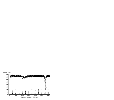
Figure 9: Intensity losses recorded as a function of the laser frequency in MHz. The peak A corresponds to a laser beam almost contra-propagating with the atoms while the peak corresponds to laser beam perpendicular to the atomic beam. The lower curve is the transmission peaks of a Fabry-Perot confocal interferometer used for frequency calibration.

We have also recorded the diffraction probability as a function of the Bragg angle, by tilting the mirror forming a standing wave. This experiment is similar to the one described inour paper miffre05 (see figure 3) but it is made with a lower power density so that only the first order diffraction appears. The diffraction is detected by measuring the intensity of the zero-order atomic beam, as shown in figure 10. Using an independent calibration of the mirror rotation as a function of the applied voltage on the piezo-actuator, we get a measurement of the Bragg angle $\theta_{B}=h/(mu\lambda_{L})=79.62\pm 0.63$ $\mu$rad corresponding to $u=1065.0\pm 8.4$ m/s.

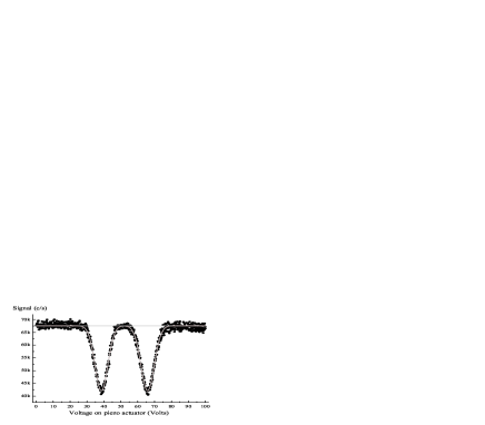
Figure 10: Plot of the intensity of the atomic beam as a function of the voltage applied on the piezoelectric actuator inducing the rotation angle of mirror $M_{2}$. When the Bragg condition is fulfilled, the direct beam intensity is reduced by diffraction in the diffraction orders $\pm 1$. The dots represent the measured intensity and the curves their best fit. In a separate experiment, we have calibrated the rotation angle as a function of the piezo voltage, $5.83\pm 0.03$ $\mu$rad/V.

These two values are very coherent and we may combine them to give our best estimate of the most probable velocity $u$:

$$u=(1065.7\pm 5.8)\mbox{m/s}$$ (21)

We can compare this measurement with the theoretical prediction for supersonic expansions. For a pure argon beam, in the limit of an infinite parallel speed ratio, theory predicts $u=\sqrt{5k_{B}T_{0}/m}$ m/s where $T_{0}$ is the nozzle temperature and $m$ the argon atomic mass. With $T_{0}=1073\pm 11$ K, we get $u=1056.7\pm 5.5$ m/s. Three small corrections must be made. We must correct for the finite value of the argon parallel speed ratio $S_{\|Ar}$, estimated to be $S_{\|Ar}=8.3$, using the semi-empirical relation of Beijerinck and Verster beijerinck81 and the associated correction reduces the most probable velocity $u$ by a fraction equal to $0.75/S_{\|Ar}^{2}\approx 1.09$% (this correction is calculated in the limit of a vanishing perpendicular temperature toennies77 ). We must replace the argon atomic mass by a weighted mean of the lithium and argon atomic masses and, with $0.86$ mbar of lithium in $167$ mbar of argon, this correction increases the velocity by $0.21$%. Finally, we must take into account the velocity slip effect: the light lithium atoms go slightly faster than the argon atoms. This difference has been calculated by numerical simulation by P. A. Skovorodko skovorodko04a and this quantity is expected to scale like $S_{\|Ar}^{2}$, so that the correction in our case is estimated to be $2.42$%. We thus predict a most probable velocity $u=1073.0\pm 5.6$ m/s, where the uncertainty comes solely from the uncertainty on the temperature $T_{0}$. This value is in satisfactory agreement with our measurements.

VI.2 The electric polarizability of lithium

Using the measured value of the most probable velocity $u$, we get the lithium electric polarizability of ⁷Li:

$$\alpha = (24.33\pm 0.16)\times 10^{-30}{\mbox{ m}}^{3}$$ (22)

$$= 164.19\pm 1.08\mbox{ atomic units}$$

The final uncertainty bar is equal to $0.66$%, resulting from the quadratic sum of the $0.54$% uncertainty on the most probable velocity $u$, the $0.2$% uncertainty on the effective length of the capacitor, the $2\times 0.15$% uncertainty due to the capacitor spacing $h_{0}$ and the $0.07$% uncertainty on the interferometric measurement. Unexpectedly, the atom interferometry result has the smallest uncertainty!

Our measurement is a mean of the polarizability of the two hyperfine sublevels $F=1$ and $F=2$ of ⁷Li. These two levels have not exactly the same polarizability. The difference $\Delta\alpha=\alpha(F=2,M_{F}=0)-\alpha(F=1,M_{F}=0)$ has been measured with great accuracy by Mowat mowat72 . We can express this result as a fraction of the mean polarisability, $\Delta\alpha=-(3.0\pm 0.1)\times 10^{-6}\alpha$. This difference is fully negligible with our present accuracy.

Our result is in excellent agreement with those of the previous measurements of $\alpha$ which are considered as being reliable. The 1934 measurement of Scheffers and Stark scheffers34 , which gave $\alpha=(12\pm 0.6)\times 10^{-30}$ m³, is generally considered to be incorrect. The first reliable measurement is due to Bederson and co-workers salop61 in 1961, who obtained $\alpha=(20.\pm 3.0)\times 10^{-30}$ m³, by using the E-H gradient balance method. In 1963, Chamberlain and Zorn chamberlain63 obtained $\alpha=(22.\pm 2.)\times 10^{-30}$ m³ by measuring the deflection of an atomic beam. Finally, in 1974, a second experiment was done by Bederson and co-workers molof74 , using the same E-H gradient balance method improved by the calibration on the polarizability of helium atom in the ${}^{3}S_{1}$ metastable state, and they obtained the value $\alpha=(24.3\pm 0.5)\times 10^{-30}$ m³.

We may also compare our measurement with theoretical results. Many calculations of $\alpha$ have been published and one can find a very complete review with 35 quotations in table 17 of the paper of King king97 published in 1997. Here is a very brief discussion of the most important results:

• the first calculation of $\alpha$ was made in 1959 by Dalgarno and Kingston dalgarno59 and gave $\alpha=165$ a.u.. This calculation was rapidly followed by several other works.

• if we forget Hartree-Fock results near $170$ a.u., a large majority of the published values are in the $162-166$ a.u. range.

• in 1994, Kassimi and Thakkar takkar94 have made a detailed study with two important results. They obtained a fully converged Hartree-Fock value, $\alpha=169.946$ a.u. and this result, far from the experimental values, proves the importance of electron correlation. They also made a series of nth-order Möller-Plesset calculations with $n=2$, $3$ and $4$, from which they extract their best estimate with an error bar, $\alpha=164.2\pm 0.1$ a.u..

• In 1996, Yan et al. yan96 have made an Hylleraas calculation, with the final value $\alpha=164.111\pm 0.002$ a.u., this value and its error bar resulting from a convergence study.

Our result is extremely close to these two very accurate calculations of $\alpha$. Two minor effects have not been taken into account in these calculations, namely relativistic correction and finite nuclear mass correction, but these two effects are quite small.

The relativistic correction on the polarizability has been studied by Lim et al. lim99 . They have made different calculations (Hartree-Fock, second order Möller-Plesset, coupled cluster CCSD and CCSD(T)) and in all cases, their relativistic result is lower than the non-relativistic result with a difference in the $0.05-0.07$ a.u. range. We do not quote here their results: even the Hartree-Fock value is lower by $0.45$ a.u. than the one of reference takkar94 , because the chosen basis set is too small.

As far as we know, no calculation of $\alpha$ has been made taking into account the finite nuclear mass. An order of magnitude of the associated correction should be given by the hydrogenic approximation: $\alpha\propto\left[1+(m/M)\right]^{3}$ and in this approximation, the polarisability of ⁷Li should be larger than its $M=\infty$ value by $0.04$ a.u. but one should not expect this approximation to predict even the sign of the correction. A high accuracy calculation of the finite mass effect is surely feasible, following the Hylleraas calculations of Yan and Drake, who have already evaluated the finite mass effect on some energies yan95a and oscillator strengths yan95b of lithium atom.

VII Conclusion

We have made a measurement of the electric polarizability of lithium atom ⁷Li by atom interferometry and we have obtained $\alpha=(24.33\pm 0.16)\times 10^{-30}{\mbox{ m}}^{3}=164.19\pm 1.08$ a.u. with a $0.66$% uncertainty. Our measurement is in excellent agreement with the most accurate experimental value obtained by Bederson and coworkers molof74 in 1974 and we have reduced the uncertainty by a factor three. Our result is also in excellent agreement with the best theoretical estimates of this quantity due to Kassimi and Thakkar takkar94 and to Yan et al. yan96 . The neglected corrections (relativistic effect, finite nuclear mass effect) should be at least ten times smaller than our present error bar.

Our measurement is the second measurement of an electric polarizability by atom interferometry, the previous experiment being done on sodium atom by D. Pritchard and co-workers ekstrom95 in 1995 (see also schmiedmayer97 and roberts04 ). This long delay is explained by the difficulty of running an atom interferometer with spatially separated beams. Using a similar experiment, J. P. Toennies and co-workers have compared the polarizabilities of helium atom and helium dimer but this work is still unpublished toennies03 .

We want now to insist on the improvements we have done with respect to the other measurement of an electric polarizability by atom interferometry, due to D. Pritchard and co-workers ekstrom95 :

• The design of our capacitor permits an analytical calculation of the $E^{2}$ integral along the atomic path. This property is important for a better understanding of the influence of small geometrical defects of the real capacitor. In the present experiment, the uncertainty on the $E^{2}$ integral is equal to $0.36$% and we think that it is possible to reduce this uncertainty near $0.1$ % with an improved construction.

• We have obtained a very good phase sensitivity of our atom interferometer: from our recordings, we estimate this phase sensitivity near $16$ mrad/$\sqrt{\mbox{Hz}}$. The accuracy achieved on phase measurement has been limited by the lack of reproducibility of the phase between consecutive recordings. We will stabilize the temperature of the rail supporting the three mirrors, hoping thus to improve the phase stability. Even if we have not been able to fully use our phase sensitivity, we have obtained set of phase-shifts measurements exhibiting an excellent consistency and accuracy, as shown by the quality of the fit of figure 8 and by the accuracy, $\pm 0.072$%, of the measurement of the quantity $\phi_{m}/V_{0}^{2}$.

• In his thesis roberts02a , T. D. Roberts reanalyzes the measurement of the electric polarizability of sodium atom made by C. R. Ekstrom et al. ekstrom95 : he estimates that a weak contribution of sodium dimers to the interference signals can be present as material gratings diffract sodium dimers as well as sodium atoms and he estimates that, in the worst case, this molecular signal might have introduced a systematic error as large as $2$% on the sodium polarizability result. Our interferometer is species selective thanks to the use of laser diffraction and this type of error does not exist in our experiment. Only lithium atoms are diffracted and even, with our choice of laser wavelength, only the ⁷Li isotope contributes to the signal.

The main limitation on the present measurement of the electric polarisability of lithium ⁷Li comes from the uncertainty on the most probable atom velocity $u$. With some exceptions, like the Aharonov-Casher phase shift aharonov84 which is independent of the atom velocity, a phase-shift induced by a perturbation is inversely proportional to the atom velocity, at least when a static perturbation is applied on one interfering beam. This is a fundamental property of atom interferometry and clever techniques are needed to overcome this difficulty:

• T. D. Roberts et al. roberts04 have developed a way of correcting the velocity dependence of the phase shift by adding another phase shift with an opposite velocity dependence. They were thus able to observe fringes with a good visibility up to very large phase shift values.

• our present results prove that a very accurate measurement can be made in the presence of an important velocity dispersion without any compensation of the associated phase dispersion, but by taking into account the velocity distribution in the data analysis.

In these two cases, one must know very accurately a velocity, the most probable velocity in our case and the velocity for which the correction phase cancels in the case of reference roberts04 . The uncertainty on this velocity may finally be the limiting factor for high precision measurements. Obviously other techniques can be used to solve this difficulty.

Finally, we think that our experiment illustrates well two very important properties of atom interferometry:

• The sensitivity of atom interferometry is a natural consequence of the well-known sensitivity of interferometry in general, which is further enhanced in the case of atom by the extremely small value of the de Broglie wavelength. Our phase measurement is in fact a direct mesaurement of the increase $\Delta v$ of the atom velocity $v$ when entering the electric field. $\Delta v$ is very simply related to the observed phase shift:

  $$\frac{\Delta v}{v}=\frac{\lambda_{dB}}{L_{eff}}\times\frac{\phi}{2\pi}$$ (23)

  This variation is extremely small, with $\Delta v/v\approx 4\times 10^{-9}$ for the largest electric field used in this experiment, corresponding to $\phi\approx 25$ rad. Our ultimate sensitivity corresponds to a phase $\phi\approx 3$ milliradian which means that we can detect a variation $\Delta v/v\approx 6\times 10^{-13}$, whereas the velocity distribution has a FWHM width equal to $21$%!

• when an atom propagates in the capacitor placed in our atom interferometer, its wavefunction samples two regions of space separated by a distance $\sim 90$ $\mu$m with a macroscopic object, the septum, lying in between and this situation extends over $75$ microsecond duration, without inducing any loss of coherence. This consequence of quantum mechanics remains very fascinating!

VIII Acknowledgements

We thank CNRS SPM and Région Midi Pyrénées for financial support. We thank P. A. Skovorodko and J. L. Heully for helpful information.

IX Appendix A: detailed calculation of the capacitor electric field

The first step is to calculate the Fourier transform $\tilde{V}(k)$ of $V(x=h,z)$ defined by equation (4):

$$\tilde{V}(k) = \frac{1}{\sqrt{2\pi}}\int_{-a}^{+a}V_{0}\exp\left(-ikz\right)dz$$ (24)

$$= \frac{2V_{0}}{\sqrt{2\pi}}\times\frac{\sin\left(ka\right)}{k}$$

The potential $V(x,z)$ given by equation (5) can then be calculated and, from $V(x,z)$, we can deduce the electric field everywhere and in particular, on the septum surface where it is parallel to the $x$-axis:

$$E_{x}(x=0,z)=\frac{1}{\sqrt{2\pi}}\int_{-\infty}^{+\infty}\tilde{V}(k)\tilde{g}(k)\exp\left(ikz\right)dk$$ (25)

with $\tilde{g}(k)=k/\sinh\left(kh\right)$. The electric field $E_{x}(x=0,z)$ is given by the inverse Fourier transform of the product of two functions $\tilde{V}(k)$ and $\tilde{g}(k)$. Therefore, the field $E_{x}(x=0,z)$ is the convolution of their inverse Fourier transforms which are $V(x=h,z)$ and $g(z)$:

$$E_{x}(x=0,z)=\int_{-\infty}^{+\infty}V(x=h,z_{1})g(z-z_{1})dz_{1}$$ (26)

Using reference gradshteyn80 (equation 6 of paragraph 4.111, p. 511), we get an explicit form of $g(z)$:

$$g(z)=\frac{\pi^{2}}{2h^{2}\cosh^{2}\left(\frac{\pi z}{2h}\right)}$$ (27)

This result proves that the field decreases asymptotically like $\exp\left(-\pi|z|/h\right)$, when $\left|z\right|-a\gg h$. We can also get a closed form expression of the electric field $E_{x}(x=0,z)$ but we may get the integral of $E^{2}$ without this result, simply by using the Parseval-Plancherel theorem and reference gradshteyn80 (equation 4 of paragraph 3.986, p. 506):

$$\int_{-\infty}^{+\infty}E_{x}(x=0,z)^{2}dz=\frac{2aV_{0}^{2}}{h^{2}}\left[\coth\left(\frac{\pi a}{h}\right)-\frac{h}{\pi a}\right]$$ (28)

The atoms sample the electric field at a small distance of the septum surface and we need the integral of $E^{2}$ along their mean trajectory. This mean trajectory is not parallel to the septum, but it is easier to calculate this integral along a constant $x$ line. From Maxwell’s equations, one gets the first correction terms to the field when $x$ does not vanish:

$$E_{x}(x,z) \approx E_{x}(x=0,z)-\frac{x^{2}}{2}\times\frac{\partial^{2}E_{x}}{\partial z^{2}}$$

$$E_{z}(x,z) \approx x\frac{\partial E_{x}}{\partial z}$$ (29)

where the derivatives are calculated for $x=0$. After an integration by parts, one gets:

$$\int_{-\infty}^{+\infty}\left[E_{x}^{2}(x,z)+E_{y}^{2}(x,z)\right]dz$$ (30)

$$= \int_{-\infty}^{+\infty}\left[E_{x}^{2}(x=0,z)+2x^{2}\left[\frac{\partial E_{x}}{\partial z}\right]^{2}\right]dz$$

where we have kept only the first non vanishing correction term in $x^{2}$. The calculation of the integral is also done with the Parseval-Plancherel theorem and, after some algebra, we get:

$$2x^{2}\int_{-\infty}^{+\infty}\left[\frac{\partial E_{x}}{\partial z}\right]^{2}dz = x^{2}\frac{V_{0}^{2}}{h^{3}}\left[\frac{2}{3}-\frac{\frac{\pi a}{h}\coth\left(\frac{\pi a}{h}\right)-1}{\sinh^{2}\left(\frac{\pi a}{h}\right)}\right]$$ (31)

$$\approx x^{2}\frac{2V_{0}^{2}}{3h^{3}}$$

where the approximate result is obtained by neglecting the exponentially small terms of the order of $\exp\left[-2\pi h/\left(a\right)\right]$.

X Appendix B: velocity average of the interference signals

We want to calculate:

$$I=I_{0}\int dvP(v)\left[1+{\mathcal{V}}_{0}\cos\left(\psi+\phi_{m}\frac{u}{v}\right)\right]$$ (32)

with the velocity distribution given by:

$$P(v)=\frac{S_{\|}}{u\sqrt{\pi}}\exp\left[-\left((v-u)S_{\|}/u\right)^{2}\right]$$ (33)

Noting $\delta=(v-u)/u$ and expanding $(u/v)$ in powers of $\delta$ up to second order, the integral becomes:

$$I/I_{0} = \frac{S_{\|}}{u\sqrt{\pi}}\int d\delta\exp\left[-\delta^{2}S_{\|}^{2}\right]$$ (34)

$$\times \left[1+{\mathcal{V}}_{0}\cos\left[\psi+\phi_{m}\left(1-\delta+\delta^{2}\right)\right]\right]$$

which can be taken exactly:

$$I/I_{0} = \left[1+\left<{\mathcal{V}}\right>\cos\left(\psi+\left<\phi\right>\right)\right]$$ (35)

$$\left<{\mathcal{V}}\right> = {\mathcal{V}}_{0}\frac{S_{\|}}{\left[S_{\|}^{4}+\phi_{m}^{2}\right]^{1/4}}\exp\left[-\frac{\phi_{m}^{2}S_{\|}^{2}}{4\left(S_{\|}^{4}+\phi_{m}^{2}\right)}\right]$$ (36)

$$\left<\phi\right> = \phi_{m}+\frac{1}{2}\arctan\left[\frac{\phi_{m}}{S_{\|}^{2}}\right]-\frac{\phi_{m}^{3}}{4\left(S_{\|}^{4}+\phi_{m}^{2}\right)}$$ (37)

We have tested this approximation by comparing this approximate formula with the result of a computer program, for a parallel speed ratio $S_{\|}=8$, corresponding to our experimental case. As shown on figure 11, the agreement is very satisfactory, at least with our present accuracy on visibility values, with differences of the order of $1$%.

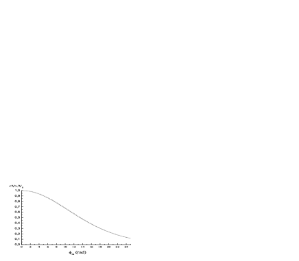
Figure 11: Calculation of the average visibility $\left<{\mathcal{V}}\right>$ in the case $S_{\|}=8$ as a function of $\phi_{m}$. The approximate result (equation 36) is plotted with a dashed line while the result of the numerical integration is plotted by the full line.

We have also studied the difference $\left(\left<\phi\right>-\phi_{m}\right)$ as a function of $\phi_{m}$ and the results are presented in figure 12. This difference can reach large values, for instance $-0.64$ rad when $\phi_{m}\approx 25$ rad. One may remark that, as obvious on equation (37), the difference $\left(\left<\phi\right>-\phi_{m}\right)$ is linear in $\phi_{m}$ and positive, when $\phi_{m}$ is small, and becomes negative and roughly cubic in $\phi_{m}$ for larger $\phi_{m}$ values. If the parallel speed ratio $S_{\|}$ is large, $S_{\|}\gg 1$, as long as the linear term is dominant, the velocity averaged phase is given by:

$$\left<\phi\right>=\phi_{m}\left[1+\frac{1}{2S_{\|}^{2}}\right]$$ (38)

and not by $\phi_{m}$. With $S_{\|}=8$, the approximate and numerical results are almost equal as long as $\phi_{m}<18$, but their difference increases rapidly for larger $\phi_{m}$ values, being close to $0.05$ radian when $\phi_{m}=25$: even if this difference is a very small fraction of $\phi_{m}$, this difference is not fully negligible and we have decided not to use the approximate analytical results (36) and (37) to fit the data.

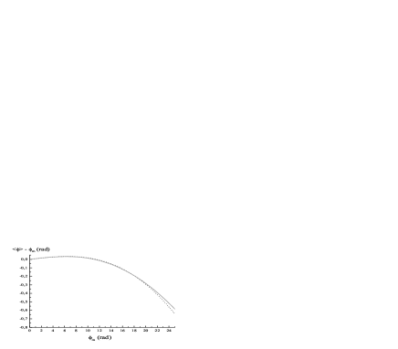
Figure 12: Calculation of the average phase $\left<\phi\right>$ in the case $S_{\|}=8$. The quantity $\left<\phi\right>-\phi_{m}$ is plotted as a function of $\phi_{m}$: dashed line for the approximate result (equation 37) and full line for the result of the numerical integration.

References

- (1) K. D. Bonin and V. V. Kresin, Electric-Dipole Polarizabilities of Atoms, Molecules and Clusters (World Scientific, 1997)
- (2) R. W. Molof, H. L. Schwartz, T. M. Miller and B. Bederson, Phys. Rev. A 10, 1131 (1974)
- (3) J. M. Amini and H. Gould, Phys. Rev. Lett. 91, 153001 (2003)
- (4) C. R. Ekstrom, J. Schmiedmayer, M. S. Chapman, T. D. Hammond and D. E. Pritchard, Phys. Rev. A 51, 3883 (1995)
- (5) R. Delhuille, C. Champenois, M. Büchner, L. Jozefowski, C. Rizzo, G. Trénec and J. Vigué, Appl. Phys. B 74, 489 (2002) 7
- (6) A. Miffre, M. Jacquey, M. Büchner, G. Trénec and J. Vigué, Eur. Phys. J. D 33, 99 (2005)
- (7) A. Miffre, M. Jacquey, M. Büchner, G. Trénec and J. Vigué, J. Chem. Phys. 122, 094308 (2005)
- (8) A. Miffre, M. Jacquey, M. Büchner, G. Trénec and J. Vigué, submitted to Phys. Rev. A; preprint available on https://hal.ccsd.cnrs.fr/ccsd-00005359
- (9) T. D. Roberts, A. D. Cronin, M. V. Tiberg and D. E. Pritchard, Phys. Rev. Lett. 92, 060405 (2004)
- (10) F. Shimizu, K. Shimizu and H. Takuma, Jpn. J. Appl. Phys. 31, L436 (1992)
- (11) S. Nowak, N. Stuhler, T. Pfau and J. Mlynek, Phys. Rev. Lett. 81, 5792 (1998)
- (12) S. Nowak, N. Stuhler, T. Pfau and J. Mlynek, Appl. Phys. B 69, 269 (1999)
- (13) V. Rieger, K. Sengstock, U. Sterr, J. H. Müller and W. Ertmer, Opt. Comm. 99, 172 (1993)
- (14) A. Morinaga, N. Nakamura, T. Kurosu and N. Ito, Phys. Rev. A 54, R21 (1996)
- (15) K. Sangster, E. A. Hinds, S. M. Barnett and E. Riis, Phys. Rev. Lett. 71, 3641 (1993)
- (16) K. Sangster, E. A. Hinds, S. M. Barnett, E. Riis and A. G. Sinclair, Phys. Rev. A 51, 1776 (1995)
- (17) K. Zeiske, G. Zinner, F. Riehle and J. Helmcke, Appl. Phys. B 60, 295 (1995)
- (18) Y. Aharonov and A. Casher, Phys. Rev. Lett. 53, 319 (1984)
- (19) Laser Cheval, website: http://www.cheval-freres.fr
- (20) D. W. Keith, C. R. Ekstrom, Q. A. Turchette and D. E. Pritchard, Phys. Rev. Lett. 66, 2693 (1991)
- (21) J. Schmiedmayer, M. S. Chapman, C. R. Ekstrom, T. D. Hammond, D. A. Kokorowski, A. Lenef, R. A. Rubinstein, E. T. Smith and D. E. Pritchard, in Atom interferometry edited by P. R. Berman (Academic Press 1997), p 1
- (22) D.M. Giltner, R. W. McGowan and Siu Au Lee, Phys. Rev. Lett. 75, 2638 (1995)
- (23) H. C. W. Beijerinck and N. F. Verster, Physica 111C, 327 (1981)
- (24) J. P. Toennies and K. Winkelmann, J. Chem. Phys. 66, 3965 (1977)
- (25) H. Haberland, U. Buck and M. Tolle, Rev. Sci. Instrum. 56, 1712 (1985)
- (26) P. A. Skovorodko, 24th International Symposium on Rarefied Gas Dynamics, AIP Conference Proceedings 762, 857 (2005) and private communication.
- (27) J. R. Mowat, Phys. Rev. A 5, 1059 (1972)
- (28) H. Scheffers and J. Stark, Phys. Z. 35, 625 (1934)
- (29) A. Salop, E. Pollack and B. Bederson, Phys. Rev. 124, 1431 (1961)
- (30) G. E. Chamberlain and J. C. Zorn, Phys. Rev. 129, 677 (1963)
- (31) F. W. King, J. Mol. Structure (Theochem) 400, 7 (1997)
- (32) A. Dalgarno and A. E. Kingston, Proc. Roy. Soc. 73, 455 (1959)
- (33) N. E. Kassimi and A. J. Thakkar, Phys. Rev. A 50, 2948 (1994)
- (34) Z. C. Yan, J. F. Babb, A. Dalgarno and G. W. F. Drake, Phys. Rev. A 54, 2824 (1996)
- (35) I. S. Lim, M. Pernpointer, M. Seth, J. K. Laerdahl, P. Schwerdtfeger, P. Neogrady and M. Urban, Phys. Rev. A 60 2822 (1999)
- (36) Z. C. Yan and G. W. F. Drake, Phys. Rev. A 52, 3711 (1995)
- (37) Z. C. Yan and G. W. F. Drake, Phys. Rev. A 52, R4316 (1995)
- (38) T. D. Roberts, Ph. D. thesis (unpublished), MIT (2002)
- (39) J. P. Toennies, private communication (2003)
- (40) I. S. Gradshteyn and I. M. Ryzhik, Tables of integrals, series and products, 4th edition, Academic Press (1980)