Bell’s inequality violation for entangled generalized Bernoulli states
in two spatially separate cavities

Abstract

We consider the entanglement of orthogonal generalized Bernoulli states in two separate single-mode high-$Q$ cavities. The expectation values and the correlations of the electric field in the cavities are obtained. We then define, in each cavity, a dichotomic operator expressible in terms of the field states which can be, in principle, experimentally measured by a probe atom that “reads” the field. Using the quantum correlations of couples of these operators, we construct a Bell’s inequality which is shown to be violated for a wide range of the degree of entanglement and which can be tested in a simple way. Thus the cavity fields directly show quantum non-local properties. A scheme is also sketched to generate entangled orthogonal generalized Bernoulli states in the two separate cavities.

I Introduction

Quantum entanglement of spatially separate systems is at the origin of non-local behavior Einstein et al. (1935); Mandel and Wolf (1995); Preskill (1998). Bell’s inequalities Bell (1964); Clauser et al. (1969) show in fact that, if the degree of entanglement is large enough, quantum correlations are incompatible with the ones due to the so-called local hidden variable theories. Experimental evidence supports quantum theory, as it was first shown by Aspect et al. (1982a, b) using entangled travelling photons and more recently by Moehring et al. (2004) using an hybrid atom-photon entanglement.

In the context of cavity quantum electrodynamics (CQED) several schemes, based on typical atom-cavity interactions, have been proposed for the production, in two separate single-mode cavities, of entangled number states of the kind $a|1_{1}1_{2}\rangle+b|0_{1}0_{2}\rangle$ Bergou and Hillery (1997), or $a|1_{1}0_{2}\rangle+b|0_{1}1_{2}\rangle$ Meystre (1992); Browne and Plenio (2003); Messina (2002); Napoli et al. (2003), where $0_{j},1_{j}$ ($j=1,2$) indicates the number of photons in the cavity $j$ and $|a|^{2}+|b|^{2}=1$. In spite of this, there are few proposals to test Bell’s inequalities for such entangled cavity fields and an experimental test has not yet been made. One of these proposals exploits an indirect method, the entanglement to be brought to light being transferred to probe atoms, for which Bell’s inequality is tested in terms of atomic pseudo-spin operators Gerry (1996). In this case one finds that atomic non-locality stands from the initial non-locality of the cavity photon system. Another proposal consists in a direct non-locality test for entangled cavity fields Kim and Lee (2000) in which Bell’s inequality to be tested is formed with parity field operators Banaszek and Wódkiewicz (1998, 1999). Within this test, classical driving fields are coupled with the two cavities where a nonlocal state has been already prepared. A couple of independent two-level atoms is then sent through the cavities and each atom off-resonantly interacts with the respective cavity field. After going out of the cavities, the atomic states are conditionally measured and Bell’s inequality can be tested by the joint probabilities of the two-level atoms being both in their excited or ground state.

The aim of this paper is to propose a direct test of Bell’s inequality for entangled fields in two spatially separate single-mode cavities using appropriate measurable cavity field operators simply implementable by the usual resonant atom-cavity interactions. It is of particular relevance to aim at getting entanglement between electromagnetic field states having mesoscopic characteristics, since in such a condition the classical-quantum border may be investigated. To this end, as well as in the context of our procedure, it is strategic to start up with entangled two-cavities electromagnetic fields exhibiting a non-zero mean field in each cavity and resulting from the passage of few resonant two-level atoms through both cavities. The reason is that, for such states, one expects to find out correlations between the non-zero fields of the two cavities. Quantum states of the electromagnetic field which satisfy these requirements are, for example, the binomial states Stoler et al. (1985); Moussa and Baseia (1998). In this paper we consider the entangled state of two separate single-mode cavities both filled with a “generalized Bernoulli state” (GBS), which is a particular case of a one-excitation generalized binomial state Stoler et al. (1985), briefly discussing a possible way to realize it experimentally. We study the expectation values and the correlations of the electric field for this entangled two-cavities state, finding, as expected, non-zero values. In such a condition, it is useful to define, in each cavity, a dichotomic operator (eigenvalues $\pm 1$) expressible in terms of the cavity field states and experimentally measurable, in principle, with the help of a resonant probe atom. We then construct a Bell’s inequality involving the correlations get established between these dichotomic operators, discussing wether and how it may be violated by the entanglement injected into the two-cavities system. We moreover suggest a simple test of this Bell’s inequality violation.

This paper is organized as follows: in Sec.II we introduce the entanglement of GBSs in two separate cavities; in Sec.III we study the expectation values and the correlations of the electric field for this entangled state; in Sec.IV we introduce the dichotomic cavity operator by which we prove the violation of Bell’s inequality, suggesting a simple experimental test, too; in Sec.V we suggest a way to generate entangled GBSs in two separate high-$Q$ single-mode cavities and we briefly discuss the potential experimental errors involved in this scheme; in Sec.VI we summarize our conclusions.

II Entanglement of orthogonal generalized Bernoulli states

The single-mode binomial state of the electromagnetic field was introduced by Stoler et al. (1985) and its principal properties are reported in literature Stoler et al. (1985); Vidiella-Barranco and Roversi (1994). Here we are interested in the particular “generalized binomial state” Stoler et al. (1985) where two consecutive number states have the same relative phase $\phi$, defined as

$$|N,p,\phi\rangle\equiv\sum_{n=0}^{N}\left[{N\choose n}p^{n}(1-p)^{N-n}\right]^{1/2}e^{in\phi}|n\rangle,$$ (1)

where $N$ is the maximum number of photons of the field, $p\in]0,1[$ is the probability of a single photon occurrence, $\phi$ is the mean phase Vidiella-Barranco and Roversi (1994) and ${N\choose n}=N!/[(N-n)!n!]$ is the Newton binomial. This state is clearly normalized. Some useful properties of the binomial state of Eq. (1) are given in App.A, where in particular we prove the orthogonality condition for two binomial states with the same $N$. More in detail, we find that two binomial states $|N,p,\phi\rangle$ and $|N,1-p,\pi+\phi\rangle$ satisfy the condition given in Eq. (56) and they are orthogonal. In the particular case $N=1$, the generalized binomial state $|1,p,\phi\rangle\equiv|p,\phi\rangle$ is called “generalized Bernoulli state” (GBS) Stoler et al. (1985).

Let us now suppose that two identical separate single-mode cavities, namely 1 and 2, are prepared in an entangled state of the form

$$|\Psi\rangle = \mathcal{N_{\eta}}\big{[}|p_{1},\vartheta_{1}\rangle_{1}|1-p_{2},\pi+\vartheta_{2}\rangle_{2}$$ (2)

$$+ \eta|1-p_{1},\pi+\vartheta_{1}\rangle_{1}|p_{2},\vartheta_{2}\rangle_{2}\big{]},$$

where $\eta$ is real, ${\cal N}_{\eta}$ is a normalization constant and the state $|p_{j},\vartheta_{j}\rangle_{j}$ ($j=1,2$) indicates that the cavity $j$ is in a GBS with probability of a single photon occurrence $p_{j}$ and mean phase $\vartheta_{j}$. The GBSs relating to the same cavity of Eq. (2) satisfy the orthogonality condition given in Eq. (56), so the state $|\Psi\rangle$ of Eq. (2) represents an entanglement of orthogonal GBSs in two spatially separate cavities and the normalization constant is

$${\cal N}_{\eta}=1/\sqrt{1+|\eta|^{2}}.$$ (3)

Using the property given in Eq. (55), we observe that, for limit values of $p_{1},p_{2}$, the entangled state of Eq. (2) becomes

$$|\Psi\rangle_{p_{1}=p_{2}=1}={\cal N_{\eta}}[|1_{1}0_{2}\rangle+\eta e^{i(\vartheta_{2}-\vartheta_{1})}|0_{1}1_{2}\rangle]$$ (4a)

$$|\Psi\rangle_{p_{1}=1,p_{2}=0}={\cal N_{\eta}}[|1_{1}1_{2}\rangle-\eta e^{-i(\vartheta_{1}+\vartheta_{2})}|0_{1}0_{2}\rangle]$$ (4b)

that is the entanglement of GBSs reduces to the entanglement of number states $|0\rangle,|1\rangle$.

In the following, we shall consider the entangled orthogonal GBSs of Eq. (2) as the injected state in the two cavities and we shall study, in this state, expectation values and correlations of the electric field and Bell’s inequality violations.

III Expectation values and correlations of the electric field

In this section we proceed to calculate both the expectation value of the electric field in the GBS of a single cavity and the correlations of the electric fields in the entangled GBSs of the two cavities defined in Eq. (2). We analyze the dependance of the correlations on the values of the system variables. Since we are considering single-mode electromagnetic fields of frequency $\omega$ inside cavities of volume $V$, the quantized electric field inside each cavity $j$ ($j=1,2$), at the time $t_{j}=0$, can be written as $\hat{\bm{E}}_{j}(z_{j})=\bm{\epsilon}_{j}\hat{E}_{j}(z_{j})$, where Vidiella-Barranco and Roversi (1994)

$$\hat{E}_{j}(z_{j})=\sqrt{\frac{4\pi\hbar\omega}{V}}(a_{j}+a_{j}^{\dagger})\sin(kz_{j}).$$ (5)

To obtain simple quantitative results, from now on we shall consider the electric field defined in Eq. (5) at the time $t_{j}=0$ in the center of the cavity, where $\sin(kz_{j})=1$.

We first calculate the matrix elements in the cavity $j$ of $\hat{E}_{j}$ in the basis of the two orthogonal GBSs $|p_{j},\vartheta_{j}\rangle$ (state 1) and $|1-p_{j},\pi+\vartheta_{j}\rangle$ (state 2). Using Eqs. (5) and (54), we obtain

$$\langle\hat{E}_{j}\rangle_{11} = -\langle\hat{E}_{j}\rangle_{22}=2\sqrt{\frac{4\pi\hbar\omega p_{j}(1-p_{j})}{V}}\cos\vartheta_{j}$$

$$\langle\hat{E}_{j}\rangle_{12} = \sqrt{\frac{4\pi\hbar\omega}{V}}[(2p_{j}-1)\cos\varphi_{j}-i\sin\vartheta_{j}].$$ (6)

The diagonal matrix element $\langle\hat{E}_{j}\rangle_{11}$ represents the expectation value of the electric field in the GBS $|p_{j},\vartheta_{j}\rangle$ and in general it differs from zero.

Using Eq. (6), we now calculate the expectation value of the electric field in each cavity $j$ for the entangled GBSs of Eq. (2), given by $\langle\hat{E}_{j}\rangle_{\Psi}\equiv\langle\Psi|\hat{E}_{j}|\Psi\rangle$. At the time $t_{j}=0$ and in the center of the cavity, we find

$$\langle\hat{E}_{j}\rangle_{\Psi}=2(-1)^{j-1}\sqrt{\frac{4\pi\hbar\omega p_{j}(1-p_{j})}{V}}\frac{1-|\eta|^{2}}{1+|\eta|^{2}}\cos\vartheta_{j}.$$ (7)

It is immediate to note that, when the entanglement is non-maximal, that is for $|\eta|\neq 1$, and when $p_{1},p_{2}\neq 0,1$ and $\vartheta_{1},\vartheta_{2}\neq\pm\pi/2$, the expectation value of the electric field of Eq. (7) differs from zero. On the other hand, for $p_{1},p_{2}=0,1$, i.e. when the entanglement is between number states, as given in Eqs. (4), we find that the expectation value of the electric field in each cavity is always equal to zero for any value of $\eta$. From Eq. (7) we also obtain that, if $|\eta|=1$, i.e. if the entanglement of Eq. (2) is maximal, the mean electric field in each cavity vanishes, as it is expected. The correlation function of the electric fields in the two cavities is given by $\langle\hat{E}_{1}\hat{E}_{2}\rangle_{\Psi}$, and using Eqs. (2) and (5) we obtain

$$\langle\hat{E}_{1}\hat{E}_{2}\rangle_{\Psi}=\frac{8\pi\hbar\omega}{V}\bigg{\{}\frac{\eta}{1+|\eta|^{2}}\big{[}f(p_{1},p_{2})\cos\vartheta_{1}\cos\vartheta_{2}$$

$$+\sin\vartheta_{1}\sin\vartheta_{2}\big{]}-h(p_{1},p_{2})\cos\vartheta_{1}\cos\vartheta_{2}\bigg{\}}$$ (8)

where we have set

$$f(p_{1},p_{2}) \equiv (2p_{1}-1)(2p_{2}-1)$$ (9a)

$$h(p_{1},p_{2}) \equiv 2\sqrt{p_{1}p_{2}(1-p_{1})(1-p_{2})}.$$ (9b)

A quantitative indication of the electric field correlations is given by the covariance

$$\mathcal{C}(\hat{E}_{1},\hat{E}_{2})=\langle\hat{E}_{1}\hat{E}_{2}\rangle_{\Psi}-\langle\hat{E}_{1}\rangle_{\Psi}\langle\hat{E}_{2}\rangle_{\Psi}.$$ (10)

From Eqs. (7) and (8), we find that the covariance for the entangled state of Eq. (2) is

$$\mathcal{C}(\hat{E}_{1},\hat{E}_{2}) = \frac{8\pi\hbar\omega}{V}\bigg{\{}\frac{\eta}{1+|\eta|^{2}}\big{[}f(p_{1},p_{2})\cos\vartheta_{1}\cos\vartheta_{2}$$ (11)

$$+ \sin\vartheta_{1}\sin\vartheta_{2}\big{]}-\left[1-\left(\frac{1-|\eta|^{2}}{1+|\eta|^{2}}\right)^{2}\right]$$

$$\times h(p_{1},p_{2})\cos\vartheta_{1}\cos\vartheta_{2}\bigg{\}}.$$

${\cal C}(\hat{E}_{1},\hat{E}_{2})$ is in general different from zero, and it vanishes when $\eta=0,\pm\infty$, i.e. when the entangled state $|\Psi\rangle$ of Eq. (2) becomes a simple product of two uncorrelated GBSs.

We now consider the covariance of Eq. (11) for some particular values of the system variables. For $\eta=\pm 1$ and $p_{1}=p_{2}=1/2$ we have

$$\mathcal{C}_{\eta=\pm 1;p_{1}=p_{2}=1/2}(\hat{E}_{1},\hat{E}_{2})=-\frac{4\pi\hbar\omega}{V}\cos(\vartheta_{1}\pm\vartheta_{2})$$ (12)

which show the importance of the values of the phase angles relations $\vartheta_{1}\pm\vartheta_{2}$. In fact, if $\vartheta_{1}\pm\vartheta_{2}=\pi/2$, the covariance of Eq. (12) vanishes; if instead $\vartheta_{1}\pm\vartheta_{2}=0$, the covariance of Eq. (12) would be equal to the maximum value $-4\pi\hbar\omega/V$.

The electric field covariance for maximally entangled number states of the form given in Eqs. (4) is obtained by setting $\eta=\pm 1$, with $p_{1}=p_{2}=1$ or $p_{1}=1,p_{2}=0$ in Eq. (11). Then we find

$$\mathcal{C}_{\eta=\pm 1;p_{1}=p_{2}=1}(\hat{E}_{1},\hat{E}_{2})=\pm\frac{4\pi\hbar\omega}{V}\cos(\vartheta_{1}-\vartheta_{2})$$ (13a)

$$\mathcal{C}_{\eta=\pm 1;p_{1}=1,p_{2}=0}(\hat{E}_{1},\hat{E}_{2})=\mp\frac{4\pi\hbar\omega}{V}\cos(\vartheta_{1}+\vartheta_{2}).$$ (13b)

From Eqs. (13) it results that the electric field covariances for the maximally entangled number states of Eqs. (4), differs from zero and they have the same absolute value of that one of Eq. (12), relating to the entangled GBSs of Eq. (2).

So, the electric fields in two separate cavities prepared in an entangled state of the form given in Eqs. (2), (4), are correlated. However, since the cavity electric fields are not easily measurable Haroche (1992), we cannot acquire any direct information about non-locality by the electric field correlations. Thus, it appears to be necessary introducing a measurable cavity operator to test non-locality of entangled cavity fields.

IV Bell’s inequality

In view of the previous considerations, in this section we shall approach the problem of non-locality for entangled fields in two spatially separate cavities, by looking if it is possible to test the property of non-locality directly for the entangled cavity field state of Eq. (2). For this purpose, we shall utilize the Clauser-Horne-Shimony-Holt (CHSH) form of Bell’s inequality Clauser et al. (1969); Mandel and Wolf (1995) which states that according to any local hidden variable theory the correlations of two dichotomic observables $A_{1}(a_{1}),A_{2}(a_{2})$ relative to two correlated subsystems $1,2$, characterized by the parameters $a_{1},a_{2}$ and whose measurement can have only two possible outcomes labelled $\pm 1$, must satisfy the following inequality

$$S_{B} \equiv |\langle A_{1}(a_{1})A_{2}(a_{2})\rangle-\langle A_{1}(a_{1})A_{2}(a^{\prime}_{2})\rangle|$$ (14)

$$+ |\langle A_{1}(a^{\prime}_{1})A_{2}(a_{2})\rangle+\langle A_{1}(a^{\prime}_{1})A_{2}(a^{\prime}_{2})\rangle|\leq 2$$

where $S_{B}$ is called Bell’s function.

IV.1 Dichotomic field operator

To test the CHSH form of Bell’s inequality defined in Eq. (14) for the cavity field entanglement of Eq. (2), one must choose the appropriate operator which correspond to the observable to be measured.

Let us first consider one single-mode cavity. Utilizing the GBS $|p,\phi\rangle$ and the orthogonal GBS $|1-p,\pi+\phi\rangle$, we introduce the dichotomic operator $\hat{F_{p}}(\phi)$, acting on the field mode and characterized by the field parameters $p,\phi$, defined as

$$\hat{F_{p}}(\phi)\equiv|p,\phi\rangle\langle p,\phi|-|1-p,\pi+\phi\rangle\langle 1-p,\pi+\phi|.$$ (15)

This operator has eigenvalues $\pm 1$ for any values of the parameters $p,\phi$ and its corresponding expression in the Fock space basis is

$$\hat{F_{p}}(\phi) = (2p-1)\left(|1\rangle\langle 1|-|0\rangle\langle 0|\right)$$ (16)

$$+ 2\sqrt{p(1-p)}\left(e^{i\phi}|1\rangle\langle 0|+e^{-i\phi}|0\rangle\langle 1|\right).$$

We shall test Bell’s inequality of Eq. (14) using the operators $\hat{F_{p}}(\phi)$, for each cavity, with different phases $\phi$ but with the same $p$. The matrix representation of $\hat{F_{p}}(\phi^{\prime})$, in the basis $\mathcal{B}_{p,\phi}=\{|p,\phi\rangle,|1-p,\pi+\phi\rangle\}$ of two orthogonal GBSs, is

$$\hat{F_{p}}(\phi^{\prime})=\left(\begin{array}[]{lr}F_{11}&F_{12}\\ F_{12}^{\ast}&-F_{11}\end{array}\right),$$ (17)

where, using Eqs. (16) and (54), the matrix elements $F_{11},F_{12}$ have the explicit expressions

$$F_{11} = \langle p,\phi|\hat{F_{p}}(\phi^{\prime})|p,\phi\rangle$$

$$= 1-8p(1-p)\sin^{2}\big{(}(\phi^{\prime}-\phi)/2\big{)};$$

$$F_{12} = \langle p,\phi|\hat{F_{p}}(\phi^{\prime})|1-p,\pi+\phi\rangle$$ (18)

$$= 2\sqrt{p(1-p)}\big{[}2(1-2p)\sin^{2}\big{(}(\phi^{\prime}-\phi)/2\big{)}$$

$$\hskip 52.63777pt+\ i\sin(\phi^{\prime}-\phi)\big{]}.$$

The matrix of Eq. (17) has clearly eigenvalues $\pm 1$, in fact

$$\lambda^{2}=F_{11}^{2}+|F_{12}|^{2}=1\Rightarrow\lambda=\pm 1.$$ (19)

The corresponding eigenstates $|p,\phi^{\prime}\rangle,|1-p,\pi+\phi^{\prime}\rangle$ of the operator $\hat{F_{p}}(\phi^{\prime})$ of Eq. (17), expressed in the basis $\mathcal{B}_{p,\phi}$, result to be

$$|1,p,\phi^{\prime}\rangle = \frac{1}{\mathcal{N}_{F}}\bigg{[}|F_{12}||1,p,\phi\rangle$$

$$+ \frac{(1-F_{11})|F_{12}|}{F_{12}}|1,1-p,\pi+\phi\rangle\bigg{]},$$

$$|1,1-p,\pi+\phi^{\prime}\rangle = \frac{1}{\mathcal{N}_{F}}\bigg{[}\frac{(F_{11}-1)|F_{12}|}{F_{12}^{\ast}}|1,p,\phi\rangle$$ (20)

$$+ |F_{12}||1,1-p,\pi+\phi\rangle\bigg{]},$$

where the normalization constant $\mathcal{N}_{F}$ is given by

$$\mathcal{N}_{F}=\sqrt{|F_{12}|^{2}+(1-F_{11})^{2}}.$$ (21)

In subsection IV.3 we will show that the operator $\hat{F_{p}}(\phi)$ defined in Eq. (15), with $p$ fixed and for different values of $\phi$, is an observable, i.e. its eigenvalues are experimentally measurable.

IV.2 Bell’s inequality violation

Let us consider the entangled GBSs introduced in Eq. (2) and for the sake of simplicity set

$$p_{1}=p_{2}=p,\quad\vartheta_{1}=\vartheta_{2}=\vartheta.$$ (22)

With this choice, the entangled state of Eq. (2) takes the form

$$|\Psi\rangle = \mathcal{N_{\eta}}\big{[}|p,\vartheta\rangle_{1}|1-p,\pi+\vartheta\rangle_{2}$$ (23)

$$+ \eta|1-p,\pi+\vartheta\rangle_{1}|p,\vartheta\rangle_{2}\big{]}$$

where $\eta$ is real and ${\cal N}_{\eta}=1/\sqrt{1+|\eta|^{2}}$. The choice of Eq. (22) allows us to simplify the expressions, so to have the results in a more readable form but without loss of generality.

Substituting the observables $A_{j}(a_{j})$ of Eq. (14) with the dichotomic operators $\hat{F}_{p}^{(j)}(\phi_{j})$ ($j=1,2$ now indicates the cavity $j$) defined in Eq. (15), with a value of the probability of single photon occurrence $p$ fixed and equal to that one appearing in the entangled state given in Eq. (23), Bell’s inequality of Eq. (14) can be written as

$$S_{B} = |\langle\hat{F}_{p}^{(1)}(\phi_{1})\hat{F}_{p}^{(2)}(\phi_{2})\rangle-\langle\hat{F}_{p}^{(1)}(\phi_{1})\hat{F}_{p}^{(2)}(\phi^{\prime}_{2})\rangle|$$

$$+ |\langle\hat{F}_{p}^{(1)}(\phi^{\prime}_{1})\hat{F}_{p}^{(2)}(\phi_{2})\rangle+\langle\hat{F}_{p}^{(1)}(\phi^{\prime}_{1})\hat{F}_{p}^{(2)}(\phi^{\prime}_{2})\rangle|\leq 2.$$

The quantum correlations appearing in Eq. (LABEL:BellF) are given by

$$\langle\hat{F}_{p}^{(1)}(\phi_{1})\hat{F}_{p}^{(2)}(\phi_{2})\rangle=\langle\Psi|\hat{F}_{p}^{(1)}(\phi_{1})\hat{F}_{p}^{(2)}(\phi_{2})|\Psi\rangle$$ (25)

where $|\Psi\rangle$ is the entanglement of GBSs of Eq. (23).

Using Eqs. (18), (23) and (25), the correlation function $\langle\hat{F}_{p}^{(1)}(\phi_{1})\hat{F}_{p}^{(2)}(\phi_{2})\rangle$ is given by

$$\langle\hat{F}_{p}^{(1)}(\phi_{1})\hat{F}_{p}^{(2)}(\phi_{2})\rangle = -1+8p(1-p)\bigg{\{}\sin^{2}\frac{\phi_{1}-\vartheta}{2}+\sin^{2}\frac{\phi_{2}-\vartheta}{2}-8p(1-p)\sin^{2}\frac{\phi_{1}-\vartheta}{2}\sin^{2}\frac{\phi_{2}-\vartheta}{2}$$ (26)

$$+ \frac{\eta}{1+|\eta|^{2}}\bigg{[}4(1-2p)^{2}\sin^{2}\frac{\phi_{1}-\vartheta}{2}\sin^{2}\frac{\phi_{2}-\vartheta}{2}+\sin(\phi_{1}-\vartheta)\sin(\phi_{2}-\vartheta)\bigg{]}\bigg{\}}.$$

It depends on the probability of single photon occurrence $p$, on the phase angle $\vartheta$ characteristic of the GBSs of the entanglement $|\Psi\rangle$, on the phase angles $\phi_{j}$ of the cavity operators $\hat{F}_{p}^{(j)}(\phi_{j})$ and on the parameter of entanglement $\eta$. We also note that all arguments of the trigonometric functions of Eq. (26) are shifted of the same angle $-\vartheta$, so the angle $\vartheta$ can be arbitrarily fixed. Now we shall look for a set of values of the parameters $p,\phi_{1},\phi_{2},\phi^{\prime}_{1},\phi^{\prime}_{2},\eta$ such that a violation of Bell’s inequality of Eq. (LABEL:BellF) occurs, i.e. $S_{B}>2$.

We begin by looking for the value of $p$ which maximizes Bell’s function $S_{B}$. As $S_{B}$ is formed by correlations of the kind (26), all having the same dependence on $p$, we simply set the partial derivative relating to $p$ of the correlation functions appearing in Eq. (LABEL:BellF) equal to zero. We have

$$\frac{\partial S_{B}}{\partial p}=(1-2p)f(p,\phi_{1},\phi_{2},\phi^{\prime}_{1},\phi^{\prime}_{2},\eta)=0,$$ (27)

where $f(p,\phi_{1},\phi_{2},\phi^{\prime}_{1},\phi^{\prime}_{2},\eta)$ is a non-singular function of the system variables. So, from Eq. (27), we obtain

$$p=1/2.$$ (28)

It is possible to see that this value of $p$ corresponds to a maximum of Bell’s function $S_{B}$. For this value $p=1/2$, setting $\hat{F}_{1/2}^{(j)}(\phi_{j})\equiv\hat{F}^{(j)}(\phi_{j})$ for simplicity, the correlation function of Eq. (26) becomes

$$\langle\hat{F}^{(1)}(\phi_{1})\hat{F}^{(2)}(\phi_{2})\rangle = \frac{2\eta}{1+|\eta|^{2}}\sin(\phi_{1}-\vartheta)\sin(\phi_{2}-\vartheta)$$ (29)

$$- \cos(\phi_{1}-\vartheta)\cos(\phi_{2}-\vartheta)$$

At this point, it is useful to consider the degree of entanglement of the state $|\Psi\rangle$ of Eq. (23), defined as Abouraddy et al. (2001)

$$G^{(E)}=G^{(E)}(|\eta|)\equiv\frac{2|\eta|}{1+|\eta|^{2}}.$$ (30)

$G^{(E)}$ is invariant with respect to the substitution $|\eta|\rightarrow 1/|\eta|$, equal to zero for $|\eta|=0,+\infty$ and equal to one (maximum value) for $|\eta|=1$. Using the expression of the correlation function given in Eq. (29) and the definition of $G^{(E)}$ of Eq. (30), Bell’s function of Eq. (LABEL:BellF) can be written as

$$S_{B} = \big{|}G^{(E)}\sin(\phi_{1}-\vartheta)[\sin(\phi_{2}-\vartheta)-\sin(\phi^{\prime}_{2}-\vartheta)]$$ (31)

$$\pm \cos(\phi_{1}-\vartheta)[\cos(\phi_{2}-\vartheta)-\cos(\phi^{\prime}_{2}-\vartheta)]\big{|}$$

$$+ \big{|}G^{(E)}\sin(\phi^{\prime}_{1}-\vartheta)[\sin(\phi_{2}-\vartheta)+\sin(\phi^{\prime}_{2}-\vartheta)]$$

$$\pm \cos(\phi^{\prime}_{1}-\vartheta)[\cos(\phi_{2}-\vartheta)+\cos(\phi^{\prime}_{2}-\vartheta)]\big{|},$$

where the signs $\pm$ correspond to $\eta$ negative or positive, respectively. We show that, with $p=1/2$ and appropriate choices of the phase angles $\phi_{1},\phi_{2},\phi^{\prime}_{1},\phi^{\prime}_{2}$, Bell’s function of Eq. (31) is greater than two, $S_{B}>2$, and Bell’s inequality of Eq. (LABEL:BellF) is violated for a wide range of the degree of entanglement $G^{(E)}$. We give here the particular case where the largest possible quantum mechanical violation of Bell’s inequality occurs (maximal violation). In App.B we give another interesting particular case.

IV.2.1 Maximal violation

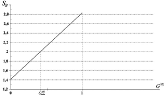
Figure 1: Maximal violation. Bell’s function $S_{B}$ vs $G^{(E)}$ with the conditions of Eq. (32) and $p=1/2$. $G_{min}^{(E)}=\sqrt{2}-1$. For $G^{(E)}=1$ we obtain the maximal violation $S_{B}^{max}=2\sqrt{2}$.

We choose the following values of the phase angles

$$\phi_{1} = \vartheta,\quad\phi_{2}=\vartheta+\pi/4,$$

$$\phi^{\prime}_{1} = \vartheta+\pi/2,\quad\phi^{\prime}_{2}=\vartheta+3\pi/4.$$ (32)

This is the standard choice of the angles for spin-$1/2$ objects to obtain the maximal violation of Bell’s inequality of the kind (14) Preskill (1998); Gerry (1996); Mandel and Wolf (1995), where the separation between two consecutive angles is $\pi/4$.

Substituting the values of the angles of Eq. (32) in Eq. (31), Bell’s function $S_{B}$ results to be

$$S_{B}=\sqrt{2}(1+G^{(E)}).$$ (33)

Using Eq. (33), we obtain that Bell’s inequality given in Eq. (LABEL:BellF) is violated, i.e. $S_{B}>2$, for those values of the degree of entanglement $G^{(E)}$ inside the interval

$$G_{min}^{(E)}<G^{(E)}\leq 1 G_{min}^{(E)}=\sqrt{2}-1\approx 0,41$$, with (34)

where $G_{min}^{(E)}$ is obtained by $S_{B}=2$. The graph of Bell’s function $S_{B}$ of Eq. (33) is plotted in Fig.1. For $G^{(E)}=1$, Bell’s function $S_{B}$ of Eq. (33) takes its maximum value

$$S_{B}(G^{(E)}=1)=S_{B}^{max}=2\sqrt{2}\approx 2,8284.$$ (35)

It is possible to prove Preskill (1998) that this is the maximal violation of Bell’s inequality.

IV.3 Test of Bell’s inequality

In this section we propose a simple scheme for testing Bell’s inequality violation shown in subsection IV.2. This test gives, in principle, a direct experimental demonstration of non-locality for the entangled GBSs in two separate cavities given in Eq. (23). We show that this test permits to measure in a simple way, for a single cavity, the eigenvalues ($\pm 1$) of the cavity operator $\hat{F}_{p}(\phi)$, by a resonant two-level probe atom which “reads” the cavity field. This result is obtained by associating the outcome of the final atomic state measurement with a given eigenvalue of the operator $\hat{F}_{p}(\phi)$. We first describe the dynamics of the resonant atom-cavity interaction.

Let $|\uparrow\rangle$ and $|\downarrow\rangle$ be respectively the excited and ground state of the probe atom with transition frequency resonant with the cavity field mode $\omega$. The dynamics of the resonant atom-cavity interaction is governed by the usual Jaynes-Cummings Hamiltonian Jaynes and Cummings (1963)

$$H_{J-C}=\frac{1}{2}\hbar\omega\sigma_{z}+\hbar\omega a^{{\dagger}}a+i\hbar g(\sigma_{+}a-\sigma_{-}a^{{\dagger}}),$$ (36)

where $g$ is the atom-field coupling constant, $a$ and $a^{{\dagger}}$ are the field annihilation and creation operators and $\sigma_{z}$, $\sigma_{+}$, $\sigma_{-}$ are the pseudo-spin atomic operators

$$\sigma_{z}=|\uparrow\rangle\langle\uparrow|-|\downarrow\rangle\langle\downarrow|,\quad\sigma_{+}=|\uparrow\rangle\langle\downarrow|,\quad\sigma_{-}=|\downarrow\rangle\langle\uparrow|.$$

The Jaynes-Cummings Hamiltonian of Eq. (36) generates the transitions Meystre (1992); Carbonaro et al. (1979)

$$|\uparrow n\rangle \rightarrow \cos(g\sqrt{n+1}t)|\uparrow n\rangle-\sin(g\sqrt{n+1}t)|\downarrow n+1\rangle$$

$$|\downarrow n\rangle \rightarrow \cos(g\sqrt{n}t)|\downarrow n\rangle+\sin(g\sqrt{n}t)|\uparrow n-1\rangle,$$ (37)

where $n$ is the number of photons inside the cavity. We ignore atomic and field dissipations during the atom-field interaction, which is a good approximation for such a systems constituted by Rydberg atoms and high-$Q$ cavities Haroche (1992).

The experimental measurement scheme is shown in Fig.2.

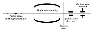
Figure 2: Experimental scheme for measuring the dichotomic field operator $\hat{F}_{p}(\phi)$ in a cavity. The atom-cavity interaction time is $T_{P}=\pi/2g$, where $g$ is the coupling constant.

A two-level probe atom is initially prepared in the ground state $|\downarrow\rangle$ and interacts on resonance with the cavity field for a time given by

$$T_{P}=\pi/2g,$$ (38)

where $g$ is the atom-field coupling constant. At this point of the sequence, utilizing the Jaynes-Cummings evolutions (37), we find the following atom-field transitions

$$|\downarrow\rangle|p,\phi\rangle \stackrel{{\scriptstyle T_{P}}}{{\rightarrow}} |0\rangle(\sqrt{1-p}|\downarrow\rangle+e^{i\phi}\sqrt{p}|\uparrow\rangle);$$

$$|\downarrow\rangle|1-p,\pi+\phi\rangle \stackrel{{\scriptstyle T_{P}}}{{\rightarrow}} |0\rangle(\sqrt{p}|\downarrow\rangle-e^{i\phi}\sqrt{1-p}|\uparrow\rangle)$$ (39)

where $|p,\phi\rangle,|1-p,\pi+\phi\rangle$ are the eigenstates of the operator $\hat{F}_{p}(\phi)$ (see Eq. (15)). Observing Eqs. (39), we note that a measurement of the atomic state after the interaction with the cavity does not allow us to distinguish the two initial eigenstates of $\hat{F}_{p}(\phi)$.

To obtain this, after going out of the cavity, we let the atom cross an opportunely set Ramsey zone where it, interacting with a classical microwave field, undergoes the transformations

$$|\uparrow\rangle \rightarrow |\uparrow\rangle_{\bm{u}}\equiv\cos(\theta/2)|\uparrow\rangle-e^{i\varphi}\sin(\theta/2)|\downarrow\rangle$$

$$|\downarrow\rangle \rightarrow |\downarrow\rangle_{\bm{u}}\equiv e^{-i\varphi}\sin(\theta/2)|\uparrow\rangle+\cos(\theta/2)|\downarrow\rangle$$ (40)

where the versor $\bm{u}$ is

$$\bm{u}\equiv(-\sin\theta\cos\varphi,-\sin\theta\sin\varphi,\cos\theta).$$ (41)

The angle $\theta\in]0,\pi[$ is the so-called “Ramsey pulse”. The values of $\theta,\varphi$ are fixed by adjusting the classical Ramsey field amplitude and the interaction time so to have

$$\cos(\theta/2)=\sqrt{p},\ \sin(\theta/2)=\sqrt{1-p};\quad\varphi=-\phi$$ (42)

where the values of $p,\phi$ are equal to the ones of the operator $\hat{F}_{p}(\phi)$ to be measured. Using Eqs. (40) together with Eqs. (42), after the Ramsey zone interaction, we find that the total atom-cavity states of Eqs. (39) undergo the following evolutions

$$|\downarrow\rangle|p,\phi\rangle \rightarrow |0\rangle e^{i\phi}|\uparrow\rangle$$ (43a)

$$|\downarrow\rangle|1-p,\pi+\phi\rangle \rightarrow |0\rangle|\downarrow\rangle.$$ (43b)

At the end of the experimental sequence of Fig.2 the atomic state is measured by field ionization detectors. From the final atom-field states of Eqs. (43) and from the definition of $\hat{F}_{p}(\phi)$ given in Eq. (15), we immediately obtain that:

• the measurement of the excited atomic state $|\uparrow\rangle$ corresponds to the eigenvalue $+1$ of $\hat{F}_{p}(\phi)$;

• the measurement of the ground atomic state $|\downarrow\rangle$ corresponds to the eigenvalue $-1$ of $\hat{F}_{p}(\phi)$.

It must be noted from Eqs. (43) that, at the end of the sequence, the cavity field state is always in the vacuum state.

Utilizing these results and the ones of subsection IV.2, we see that an experimental test of the CHSH form of Bell’s inequality of Eq. (LABEL:BellF) for the entangled GBSs in two spatially separate cavities of Eq. (23) requires the following steps:

• the generation of the entangled GBSs given in Eq. (23), with $p=1/2$ and an arbitrarily fixed $\vartheta$;

• the resonant interaction of two two-level probe atoms with their respective cavity and with a successive Ramsey zone, according to the scheme of Fig.2. The Ramsey zone interaction is set so as to have a $\pi/2$-pulse and the values of the angles $\phi_{j}$ desired (see Eq. (42)), given, for example, by the choice of Eq. (32);

• the simultaneous measurement of atomic states, each one corresponding to a given eigenvalue of the dichotomic operator $\hat{F}_{1/2}^{(j)}(\phi_{j})$, as it was found in Eqs. (43). The simultaneity of the measurements ensures that the events are “space-like” separate, so as to close the locality loophole Massar et al. (2002).

After repeating this sequence for many times, it is possible to obtain the correlations $\langle\hat{F}_{1/2}^{(1)}(\phi_{1})\hat{F}_{1/2}^{(2)}(\phi_{2})\rangle$ for the desired values of the angles $\phi_{1},\phi_{2}$ by statistical averages and then to test Bell’s inequality of Eq. (LABEL:BellF). A brief discussion on the typical experimental parameters involved in this measurement scheme is given in Sec.VI.

V Sketch of a scheme to generate entangled generalized Bernoulli states in separate cavities

As stressed at the end of the previous section, testing Bell’s inequality violation requires, as first step, the generation of entangled GBSs of Eq. (2) in the two separate single-mode cavities. In this section, following standard procedures currently implemented in laboratory to produce assigned states of the electromagnetic fields inside a cavity Haroche (1992, 2002), we sketch the main steps of a scheme, shown in Fig.3, aimed at generating in principle our target entangled state.

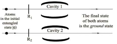
Figure 3: Experimental scheme for the generation of entangled orthogonal GBSs in two separate cavities.

Let us consider a couple of identical two-level Rydberg atoms initially in the entangled state

$$|\phi\rangle={\cal N}_{\eta}(|\uparrow_{1}\downarrow_{2}\rangle+\eta|\downarrow_{1}\uparrow_{2}\rangle),$$ (44)

where $\eta$ is real and ${\cal N}_{\eta}=1/\sqrt{1+|\eta|^{2}}$ is a normalization constant, which can be prepared using, for example, the scheme suggested by Gerry Gerry (1996) and let us also consider two identical high-$Q$ single-mode cavities each in the vacuum state $|O_{1}\rangle$, $|0_{2}\rangle$. Each atom of the entangled atomic state of Eq. (44) crosses a Ramsey zone ${\rm R}_{j}$ ($j=1,2$), where it undergoes the transformations given in Eqs. (40). If we set, for each atom $j$,

$$\cos(\theta_{j}/2)\equiv\sqrt{p_{j}},\ \sin(\theta_{j}/2)\equiv\sqrt{1-p_{j}};\ \varphi_{j}=-\vartheta_{j}$$ (45)

where $p_{1},p_{2}$ are two arbitrary real numbers inside the interval $]0,1[$, the transformations of Eqs. (40) can be written as

$$|\uparrow_{j}\rangle \rightarrow |\uparrow\rangle_{\bm{u}_{j}}\equiv\sqrt{p_{j}}|\uparrow_{j}\rangle-e^{-i\vartheta_{j}}\sqrt{1-p_{j}}|\downarrow_{j}\rangle$$

$$|\downarrow_{j}\rangle \rightarrow |\downarrow\rangle_{\bm{u}_{j}}\equiv e^{i\vartheta_{j}}\sqrt{1-p_{j}}|\uparrow_{j}\rangle+\sqrt{p_{j}}|\downarrow_{j}\rangle.$$ (46)

The total atom-cavity state after the Ramsey zones is

$$|\Psi(0)\rangle_{tot}=\mathcal{N}_{\eta}\big{(}|\uparrow\rangle_{\bm{u}_{1}}|\downarrow\rangle_{\bm{u}_{2}}+\eta|\downarrow\rangle_{\bm{u}_{1}}|\uparrow\rangle_{\bm{u}_{2}}\big{)}|0_{1}0_{2}\rangle.$$ (47)

Now, the atoms resonantly interact with their respective cavities for a time $T$ such that

$$gT=\pi/2.$$ (48)

Since the two subsystems 1 and 2 are independent, we can utilize the usual Jaynes-Cummings evolutions given in Eqs. (37) for each subsystem $j$, so that at the time $T$ the state of Eq. (47) becomes

$$|\Psi(T)\rangle_{tot} = \mathcal{N_{\eta}}\Big{[}|p_{1},\vartheta_{1}\rangle_{1}|1-p_{2},\pi+\vartheta_{2}\rangle_{2}$$

$$+ \eta|1-p_{1},\pi+\vartheta_{1}\rangle_{1}|p_{2},\vartheta_{2}\rangle_{2}\Big{]}|\downarrow_{1}\downarrow_{2}\rangle,$$

where we have omitted the unimportant global phase factor $e^{i(\pi-\vartheta_{1}-\vartheta_{2})}$ and we have used the notation of Eq. (54) for the GBSs. After the interaction, the total atom-cavity state of Eq. (LABEL:Psitotal) describes both atoms in their ground state and the cavity field state in the pure entangled state

$$|\Psi\rangle = \mathcal{N_{\eta}}\Big{[}|p_{1},\vartheta_{1}\rangle_{1}|1-p_{2},\pi+\vartheta_{2}\rangle_{2}$$ (50)

$$+ \eta|1-p_{1},\pi+\vartheta_{1}\rangle_{1}|p_{2},\vartheta_{2}\rangle_{2}\Big{]}$$

which represents the entanglement of two orthogonal GBSs of the form defined in Eq. (2). By adjusting appropriately the settings of the Ramsey zones, the values of $p_{j}$ and $\vartheta_{j}$ can be arbitrarily changed (see Eq. (45)).

Although we shall not enter into the details of the experimental feasibility of the proposed generation scheme, we shall give here a brief valuation of some potential errors involved in such a scheme. A necessary condition required by our generation scheme is that the atoms interact with the cavities for a given period of time. This can be obtained by the selection of a well determinate atomic velocity. Any experimental error $\Delta v$ in the atomic velocity $v$ induces an error $\Delta T$ in the atom-cavity interaction time $T$ given by

$$\Delta T=\bigg{|}L\Delta\bigg{(}\frac{1}{v}\bigg{)}\bigg{|}\approx\frac{L\Delta v}{v^{2}}=T\frac{\Delta v}{v},$$ (51)

where $L$ is the cavity length. From Eq. (51) we find that the velocity relative error $\Delta v/v$ must satisfy the condition

$$\frac{\Delta T}{T}\approx\frac{\Delta v}{v}\ll 1$$ (52)

in order that the time relative error $\Delta T/T$ may be negligible. In current laboratory experiments it is possible to select a given atomic velocity with a relative error $\sim 10^{-2}$ or less Hagley et al. (1997); Haroche (2002), so that, from Eq. (52), $\Delta T/T$ is of the same order.

Another aspect we have excluded is the atomic or photon decay during the atom-cavity interactions. This assumption can be held if

$$\tau_{at},\tau_{cav}>T,$$ (53)

where $\tau_{at},\tau_{cav}$ are respectively the atomic and photon mean lifetimes and $T$ is the interaction time. For Rydberg atomic levels and microwave superconducting cavities with quality factor $Q\sim 10^{8}\div 10^{10}$, we have $\tau_{at}\sim 10^{-5}\div 10^{-2}\textrm{s}$ and $\tau_{cav}\sim 10^{-4}\div 10^{-1}\textrm{s}$. Since typical atom-cavity field interaction times are $T\sim 10^{-5}\div 10^{-4}\textrm{s}$, the required condition of Eq. (53) can be satisfied Haroche (1992). Moreover, the typical mean lifetimes of the Rydberg atomic levels $\tau_{at}$ must be such that the atoms do not decay during the entire sequence of the scheme and the photon mean lifetimes $\tau_{cav}$ must be long enough to permit cavity fields not to decay before they interact with probe atoms Haroche (1992, 2002); Nogues et al. (1999), so as to allow the successive Bell’s inequality test (see subsection IV.3).

VI Conclusion

In this paper, we have considered two spatially separate single-mode cavities where it has been injected an electromagnetic field in an entangled state of two orthogonal generalized Bernoulli states (GBS). We have then studied the expectation values and the correlations of the electric fields of these two cavities, finding that they are in general different from zero. The existence of such correlations between the two cavities indicates that the fields are non-local in this system. The cavity electric fields, and so their correlations, are however not directly measurable.

To examine the non-local feature of the electromagnetic fields in the two cavities, we have introduced, for each cavity, a dichotomic operator $\hat{F_{p}}(\phi)$ with eigenvalues $\pm 1$ acting on the field states and in principle measurable. Using the quantum correlations of couples of these operators with different values of $\phi$ and with the same $p$, we have constructed the CHSH form of Bell’s inequality finding that, for opportune choices of the system variables, this Bell’s inequality is violated for a wide range of the degree of entanglement. Quantum non-locality is thus directly shown by the cavity fields in the entanglement of GBSs in two separate cavities. This remarkable feature of such an entangled state is one of our main results.

We have also proposed a simple test of this Bell’s inequality violation which exploits a couple of two-level probe atoms each interacting resonantly with the respective cavity and successively with an opportune Ramsey zone for an assigned time. Appropriate Ramsey zone settings, i.e. pulse and relative phase of the atomic states, allow the unconditional measurement of the cavity operator $\hat{F_{p}}(\phi)$. Our result is that, if each probe atom is initially in the ground state and its final state is detected at the end of the sequence, the measurement of the excited or ground state is equivalent to the eigenvalue $+1$ or $-1$ of the cavity operator, respectively. So, our Bell’s inequality test requires (i) the repeated preparation of entangled orthogonal GBSs in two separate single-mode cavities, (ii) the use of two independent probe atoms, each of them following the above experimental sequence with the desired settings of Ramsey zone, and (iii) the simultaneous measurement of the final atomic states, which is equivalent to the measurement of the eigenvalues of the introduced cavity operators. The cavity operators correlations can be then obtained by statistical averages of the eigenvalues products. This Bell’s inequality test is non-conditional and it requires that the atoms resonantly interact with the cavities for an assigned time. The main result found in this paper is that, by our procedure, it is possible to obtain in a simple way a direct verification of Bell’s inequality violation for the cavity electromagnetic fields. We wish to emphasize that our test is immune to the typical experimental errors on the desired interaction time Hagley et al. (1997); Haroche (2002). In the experimental context of the Bell’s inequality test, another important parameter to be considered is the atomic state detector efficiency $\alpha$ that we have supposed as ideal for simplicity. Had we incorporated detectors efficiencies in the correlation functions, then the CHSH form of Bell’s inequality would not have been violated for values of $\alpha$ less than $\alpha_{t}=2/(\sqrt{2}+1)\approx 0,8284$ for maximally entangled states of a bipartite system Clauser et al. (1969); Massar et al. (2002). However, also in this case, it is always possible to test the CHSH form of Bell’s inequality with the “fair sampling” hypothesis that the sub-ensemble of detected events (detected atoms) represents the whole ensemble. So, the results just rely on the detected events but the probabilistic nature of atomic detection leaves “open” the detection loophole Moehring et al. (2004); Massar et al. (2002). Only for detector efficiencies greater than $\alpha_{t}$ the detection loophole can be closed.

We conclude that, at this time, the experimental developments seem to be rather promising on the possibility of implementing our measurement scheme, so as to allow the realization of the first direct test of Bell’s inequality for entangled fields in two spatially separate cavities.

Appendix A Binomial states. Definition and some properties

In Sec.II we have given the definition of the particular generalized binomial state $|N,p,\phi\rangle$. In this paper we consider the particular case of generalized binomial states with $N=1$, i.e. the so-called “generalized Bernoulli state” (GBS) Stoler et al. (1985), whose explicit expression is

$$|p,\phi\rangle=\sqrt{1-p}|0\rangle+e^{i\phi}\sqrt{p}|1\rangle,$$ (54)

as it is readily obtained by Eq. (1). We now give some properties of the generalized binomial state $|N,p,\phi\rangle$, defined in Eq. (1), which will be useful in this paper.

i) In the limits $p=0,1$, the binomial state of Eq. (1) becomes

$$\lim_{p\rightarrow 0}|N,p,\phi\rangle=|0\rangle,\quad\lim_{p\rightarrow 1}|N,p,\phi\rangle=|N\rangle.$$ (55)

ii) Two binomial states of the kind given in Eq. (1), $|N,p,\phi\rangle,|N,p^{\prime},\phi^{\prime}\rangle$, with the same maximum number of photons $N$, are orthogonal if and only if

$$p^{\prime}=1-p\quad e\quad\phi^{\prime}=(2m+1)\pi+\phi,\ m\in\mathbb{Z}.$$ (56)

As far as we know, this orthogonality property has not been reported in literature yet, so we give here the proof.

The scalar product of two binomial states $|N,p,\phi\rangle$ and $|N,p^{\prime},\phi^{\prime}\rangle$, of the form defined in Eq. (1), is given by

$$\langle N,p,\phi|N,p^{\prime},\phi^{\prime}\rangle = \sum_{n=0}^{N}{N\choose n}(pp^{\prime})^{n/2}$$

$$\times[(1-p)(1-p^{\prime})]^{(N-n)/2}e^{in(\phi^{\prime}-\phi)}.$$

Substituting the equalities of Eq. (56) in Eq. (LABEL:scabin), we obtain

$$\langle N,p,\phi|N,1-p,\pi+\phi\rangle = [p(1-p)]^{N/2}\sum_{n=0}^{N}{N\choose n}e^{in\pi}$$ (58)

$$= [p(1-p)]^{N/2}(e^{i\pi}+1)^{N}$$

$$= 0,$$

where we have used the binomial theorem of Newton and the equality $e^{i\pi}=-1$. This proves that the conditions of Eq. (56) are sufficient. The conditions of Eq. (56) are also necessary. In fact, the scalar product of Eq. (LABEL:scabin) can be wrote

$$\langle N,p,\phi|N,p^{\prime},\phi^{\prime}\rangle = \sum_{n=0}^{N}{N\choose n}\left(e^{i(\phi^{\prime}-\phi)}\sqrt{pp^{\prime}}\right)^{n}$$

$$\times\left(\sqrt{(1-p)(1-p^{\prime})}\right)^{N-n}.$$

Utilizing the usual binomial theorem of Newton, we obtain

$$\langle N,p,\phi|N,p^{\prime},\phi^{\prime}\rangle = \Big{(}e^{i(\phi^{\prime}-\phi)}\sqrt{pp^{\prime}}$$ (59)

$$+ \sqrt{(1-p)(1-p^{\prime})}\Big{)}^{N}$$

and setting this equation equal to zero, it must be

$$e^{i(\phi^{\prime}-\phi)}\sqrt{pp^{\prime}}+\sqrt{(1-p)(1-p^{\prime})}=0.$$ (60)

Since the square roots are real and non-negative, from Eq. (60) we have

$$e^{i(\phi^{\prime}-\phi)}=-1\Leftrightarrow\phi^{\prime}-\phi=(2m+1)\pi,\ m\in\mathbb{Z}.$$ (61)

So, Eq. (60) becomes

$$\sqrt{pp^{\prime}}=\sqrt{(1-p)(1-p^{\prime})} \Rightarrow pp^{\prime}=1-p-p^{\prime}+pp^{\prime}$$ (62)

$$\Rightarrow p^{\prime}=1-p.$$

From the results of Eqs. (61), (62), we see that the orthogonality condition of Eq. (56) is proved.

Appendix B Another Bell’s inequality violation

We give here another case of violation of the CHSH form of Bell’s inequality given in Eq. (LABEL:BellF) for the entangled GBSs of Eq. (23). In this case, the interval of values of the degree of entanglement where a Bell’s inequality violation occurs is the widest obtainable.

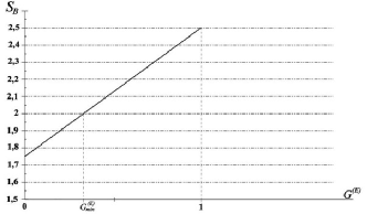
Figure 4: Bell’s function $S_{B}$ vs $G^{(E)}$ with the conditions of Eq. (65) together with $p=1/2$. $G_{min}^{(E)}=1/3$.

Let us choose the following values for the phase angles of Eq. (31)

$$\phi_{1} = \phi_{2}=\vartheta,\quad\phi^{\prime}_{1}=\vartheta+\pi/3,$$

$$\phi^{\prime}_{2} = \left\{\begin{array}[]{ll}\vartheta-2\pi/3,&\textrm{if $\eta$ is positive}\\ \vartheta+2\pi/3,&\textrm{if $\eta$ is negative}\end{array}\right.$$ (65)

With this set of values of the angles, Bell’s function $S_{B}$ of Eq. (31) becomes

$$S_{B}=\frac{7}{4}+\frac{3}{4}G^{(E)}.$$ (66)

Using Eq. (66), we find that Bell’s inequality of Eq. (LABEL:BellF) is violated, i.e. $S_{B}>2$, for those values of the degree of entanglement $G^{(E)}$ inside the interval

$$G_{min}^{(E)}<G^{(E)}\leq 1 G_{min}^{(E)}=1/3=0,\bar{3}$$, with . (67)

The value of $G_{min}^{(E)}$ is clearly obtained by the condition $S_{B}=2$. This interval of values of $G^{(E)}$, for which Bell’s inequality is violated, is the widest we found. In Fig.4 we plot the graph of Bell’s function $S_{B}$ of Eq. (66) vs the degree of entanglement $G^{(E)}$, for the choices given in Eq. (65). The maximum violation value of $S_{B}$ is obtained when $G^{(E)}=1$, i.e. when the state (23) is maximally entangled, and it is

$$S_{B}(G^{(E)}=1)=5/2=2,5.$$ (68)

References

- Einstein et al. (1935) A. Einstein, B. Podolsky, and N. Rosen, Phys. Rev. 47, 777 (1935).
- Preskill (1998) J. Preskill, Tech. Rep., California Institute of Technology (1998), http://theory.caltech.edu/preskill/ph229.
- Mandel and Wolf (1995) L. Mandel and E. Wolf, Optical Coherence and Quantum Optics (Cambridge University Press, Cambridge, New York, Melbourne, 1995).
- Bell (1964) J. S. Bell, Physics 1, 195 (1964).
- Clauser et al. (1969) J. F. Clauser, M. A. Horne, A. Shimony, and R. A. Holt, Phys. Rev. Lett. 23, 880 (1969).
- Aspect et al. (1982a) A. Aspect, P. Grangier, and G. Roger, Phys. Rev. Lett. 49, 91 (1982a).
- Aspect et al. (1982b) A. Aspect, J. Dalibard, and G. Roger, Phys. Rev. Lett. 49, 1804 (1982b).
- Moehring et al. (2004) D. L. Moehring, M. J. Madsen, B. B. Blinov, and C. Monroe, Phys. Rev. Lett. 93, 090410 (2004).
- Bergou and Hillery (1997) J. A. Bergou and M. Hillery, Phys. Rev. A 55, 4585 (1997).
- Meystre (1992) P. Meystre, in Progress in Optics XXX, Cavity Quantum Optics and the Quantum Measurement Process, edited by E. Wolf (Elsevier Science Publishers B.V., New York, 1992).
- Browne and Plenio (2003) D. E. Browne and M. B. Plenio, Phys. Rev. A 67, 012325 (2003).
- Messina (2002) A. Messina, Eur. Phys. J. D 18, 379 (2002).
- Napoli et al. (2003) A. Napoli, A. Messina, and G. Compagno, Fortschr. Phys. 51, 81 (2003).
- Gerry (1996) C. C. Gerry, Phys. Rev. A 53, 4583 (1996).
- Kim and Lee (2000) M. S. Kim and J. Lee, Phys. Rev. A 61, 042102 (2000).
- Banaszek and Wódkiewicz (1998) K. Banaszek and K. Wódkiewicz, Phys. Rev. A 58, 4345 (1998).
- Banaszek and Wódkiewicz (1999) K. Banaszek and K. Wódkiewicz, Phys. Rev. Lett. 82, 2009 (1999).
- Stoler et al. (1985) D. Stoler, B. E. A. Saleh, and M. C. Teich, Opt. Acta 32, 345 (1985).
- Moussa and Baseia (1998) M. Moussa and B. Baseia, Phys. Lett. A 238, 223 (1998).
- Vidiella-Barranco and Roversi (1994) A. Vidiella-Barranco and J. A. Roversi, Phys. Rev. A 67, 5233 (1994).
- Haroche (1992) S. Haroche, in Les Houches Session LIII 1990, Course 13, Cavity Quantum Electrodynamics (Elsevier Science Publishers B.V., New York, 1992).
- Abouraddy et al. (2001) A. F. Abouraddy, B. E. A. Saleh, A. V. Sergienko, and M. C. Teich, Phys. Rev. A 64, 050101 (2001).
- Jaynes and Cummings (1963) E. T. Jaynes and F. W. Cummings, P.I.E.E.E. 51, 89 (1963).
- Carbonaro et al. (1979) P. Carbonaro, G. Compagno, and F. Persico, Phys. Lett. A 73, 97 (1979).
- Massar et al. (2002) S. Massar, S. Pironio, J. Roland, and B. Gisin, Phys. Rev. A 66, 052112 (2002).
- Haroche (2002) S. Haroche, Phys. Scripta 102, 128 (2002).
- Hagley et al. (1997) E. Hagley et al., Phys. Rev. Lett. 79, 1 (1997).
- Nogues et al. (1999) G. Nogues, A. Rauschenbeutel, S. Osnaghi, M. Brune, J. M. Raimond, and S. Haroche, Nature (London) 400, 239 (1999).