Optimal Bell tests do not require maximally entangled states

Abstract

Any Bell test consists of a sequence of measurements on a quantum state in space-like separated regions. Thus, a state is better than others for a Bell test when, for the optimal measurements and the same number of trials, the probability of existence of a local model for the observed outcomes is smaller. The maximization over states and measurements defines the optimal nonlocality proof. Numerical results show that the required optimal state does not have to be maximally entangled.

As first shown by Bell Bell in 1964, the correlations among the measurement outcomes of space-like separated parties on some quantum states cannot be reproduced by a local theory. This fact is often referred to as quantum nonlocality and has been recognized as the most intriguing quantum feature. The fundamental importance of the work by Bell was that it provided conditions for experimentally testing Quantum Mechanics (QM) versus the whole set of local models, the so-called Bell inequalities. The experimental demonstration exp , up to some loopholes, of a Bell inequality violation definitely closed the Einstein-Podolsky-Rosen program EPR for the existence of a local theory alternative to QM.

The interest on quantum correlations, or entanglement, has dramatically increased during the last two decades due to the emerging field of Quantum Information Science (QIS) book . It has been realized that quantum states provide new ways of information processing and communication without analog in Classical Information. The essential resource for most of these applications are entangled states. This has motivated a strong effort devoted to the characterization and quantification of the entanglement of quantum states. Although many questions remain unanswered, the problem is completely solved for the case of pure states in bipartite systems. For a state $|\Psi\rangle\in{\cal H}_{A}\otimes{\cal H}_{B}$, its amount of entanglement is specified by the so-called entropy of entanglement BBPS , $E(\Psi)=S(\rho_{A})$, where $S$ is the usual von Neumann entropy and $\rho_{A}=\mbox{tr}_{B}(|\Psi\rangle\!\langle\Psi|)$. In particular, this means that the maximally entangled state in a bipartite system of dimension $d\times d$, reads

$$|\Phi_{d}\rangle=\frac{1}{\sqrt{d}}\sum_{i=1}^{d}|ii\rangle,$$ (1)

where $\{i\}$ define orthonormal bases in ${\cal H}_{A}$ and ${\cal H}_{B}$.

Apart from their importance for quantum information applications, entangled states provide the only known way of establishing nonlocal correlations among space-like separated parties. It is meant here by nonlocal those correlations that (i) cannot be explained by a local model but (ii) do not allow any faster-than-light communication, that is, they are consistent with the no-signaling condition. Indeed, it is a well-established result that a quantum pure state violates a Bell inequality if and only if it is entangled Gisin . However, it is also well known that there exist nonlocal correlations that are not achievable by measuring quantum states PR . In a similar line of thought, it has very often been assumed that $|\Phi_{d}\rangle$ represents the most nonlocal quantum state too. However, no precise demonstration of this fact has ever been given and, indeed, it is one of the scopes of this work to raise some doubts about this statement.

In what follows, entangled states constitute a resource for constructing nonlocality proofs. The strength of a Bell experiment has to be computed by means of statistical tools: a Bell test is better than another when, for the same number of trials, the probability that a local model explains the observed outcomes is smaller. Recall that statistical fluctuations on finite samples allow a local theory to predict the possibility of data violating a Bell inequality. The goal is then to identify those states needed in the construction of optimal Bell tests. The importance of constructing optimal nonlocality proofs is two-fold. First, from an experimental point of view, they allow improving present Bell experiments, especially in terms of the needed resources. Second, Bell tests also represent an important tool for QIS useful . In particular, they are useful for testing the quantumness of devices. This is a hardly explored problem in QIS that, for instance, can be especially relevant in cryptographic applications MY : given some observed correlations among several parties, how can its quantum origin be certified? Could these correlations have alternatively been established by classical means, i.e. shared randomness? Bell inequalities provide an answer to the previous questions.

The scenario: We consider the standard scenario for any Bell test. Two space-like separated parties, called Alice and Bob, share copies of a pure quantum state $|\Psi\rangle\in{\cal H}_{A}\otimes{\cal H}_{B}$, of dimension $d\times d$. They can choose among $m$ possible measurements, each of $n$ outcomes, this being denoted by $m\times n$. $A_{j}^{i}$ denotes the positive operator corresponding to the outcome $j$ of the measurement $i$ for Alice, so $\sum_{j}A_{j}^{i}=\leavevmode\hbox{\small 1\normalsize\kern-3.30002pt1}$. Similarly, Bob’s measurement operators are denoted by $B_{j}^{i}$. The probability that Alice and Bob obtain the outcomes $j_{A}$ and $j_{B}$ after applying the measurement $i_{A}$ and $i_{B}$, where $j_{A},j_{B}=1,\ldots,n$ and $i_{A},i_{B}=1,\ldots,m$, on $|\Psi\rangle$ is

$$p_{Q}(j_{A},j_{B}|i_{A},i_{B})=\mbox{tr}\left(A_{j_{A}}^{i_{A}}\otimes B_{j_{B}}^{i_{B}}|\Psi\rangle\!\langle\Psi|\right).$$ (2)

In a Bell experiment, a quantum state is prepared and sent to the parties who measure it. After $N$ repetitions of the experiment, the frequencies of the results define a $(m^{2}n^{2})$-dimensional vector whose components tend to $p_{Q}(j_{A},j_{B}|i_{A},i_{B})$ when $N\rightarrow\infty$. A vector of probabilities is achievable using QM when there exist a state $|\Psi\rangle$ and measurements $A_{j_{A}}^{i_{A}}$ and $B_{j_{B}}^{i_{B}}$ satisfying (2).

On the other hand, in a local model any observed correlation between measurement results in space-like separated regions should come from initially shared random data, denoted by $\lambda$. QM is nonlocal because some of the vectors (2) do not allow a local description, i.e. they cannot be written as

$$p_{L}(j_{A},j_{B}|i_{A},i_{B})=\sum_{\lambda}p\,(\lambda)p\,(j_{A}|i_{A},\lambda)p\,(j_{B}|i_{B},\lambda).$$ (3)

Therefore, shared quantum states can be used to establish nonlocal correlations.

The goal of any Bell experiment is to test the hypothesis ${\cal Q}$, “the observed outcomes are governed by a quantum probability distribution (2)”, against the composite hypothesis ${\cal L}$, “there exists a local model (3) reproducing the data” vDGG . The statistical tool that quantifies the average amount of support in favor of ${\cal Q}$ against ${\cal L}$ per trial when the data are generated by ${\cal Q}$ is the so-called relative entropy or Kullback-Leibler (KL) Divergence CT , $D$. For two probability distributions, $\vec{p}_{1}$ and $\vec{p}_{2}$ associated to the event $\{z\}$, it reads

$$D(\vec{p}_{1}||\vec{p}_{2})=\sum_{z}p_{1}(z)\log(p_{1}(z)/p_{2}(z)).$$ (4)

We denote by $\vec{q}=(q(1,1,1,1),\ldots,q(m,m,n,n))$ the quantum probabilities for the measurement settings $i_{A}$ and $i_{B}$, and outcomes $j_{A}$ and $j_{B}$. Using (2), one has

$$q(i_{A},i_{B},j_{A},j_{B})=\mbox{tr}\left(A_{j_{A}}^{i_{A}}\otimes B_{j_{B}}^{i_{B}}|\Psi\rangle\!\langle\Psi|\right)p_{M}(i_{A},i_{B}),$$ (5)

where $p_{M}(i_{A},i_{B})$ characterizes the choice of measurements by Alice and Bob. Now, the support in favor of ${\cal Q}$ against ${\cal L}$ provided by these quantum data is vDGG

$$D({\cal Q}||{\cal L})=\min_{\vec{p}\in{\cal L}}D(\vec{q}\,||\vec{p}),$$ (6)

where the minimization runs over all alternative local models, $\vec{p}$. The vector $\vec{p}$ is defined analogously to (5), replacing the quantum term $p_{Q}$ (2) by a local model $p_{L}$ (3). This quantity gives the statistical figure of merit to be maximized in any nonlocality test vDGG . It is worth mentioning here that the KL Divergence (i) is an asymptotic measure and (ii) appears as the measure of statistical support for the two most commonly used methods for hypothesis testing, frequentist and Bayesian (see vDGG for more details). Moreover, and despite not being symmetric, it can be seen as a measure of statistical distance between probability distributions.

It is often convenient to interpret a Bell test as a game between a quantum and a local player vDGG ; Peres . The quantum player has to design an experimental situation for which the local player is unable to provide a model. Thus, the quantum player looks for the experiment that gives him the victory with the minimal number of repetitions, i.e. his task consists of designing the Bell test maximizing (6). In order to do that, he can choose the state to be prepared, the measurements, and the probability governing the choice of measurements, $p_{M}(i_{A},i_{B})$. Notice that we do not impose $p_{M}(i_{A},i_{B})$ to be product. Indeed, one could think of a configuration where an external referee is sending the choice of measurements to the parties. On the other hand, the local player only assumes the existence of a local model. In particular, he is allowed to change his description according to the observed data.

Results: In what follows, the optimality of Bell tests is analyzed according to the KL Divergence. The optimization of (6) in full generality is a very hard problem. Here, we mainly consider the standard situation where Alice and Bob apply two projective measurements, i.e. $m=2$, $n=d$ and $A_{i}^{j}$ and $B_{i}^{j}$ are mutually orthogonal one-dimensional projectors. For a fixed number of measurements, it is possible to search numerically the state and measurements defining the optimal Bell test. In the qubit case, $d=2$, the best nonlocality proof is given by the maximally entangled state $|\Phi_{2}\rangle$ (1) and the measurements maximizing the violation of the CHSH inequality CHSH , as expected. The KL Divergence turns out to be equal to 0.046 bits vDGG and the optimal choice of settings is completely random, $p_{M}(i_{A},i_{B})=1/4$. Actually, the optimal choice of settings turns out to be random for all the situations considered in this work.

Moving to higher dimension, the optimal measurements for the maximally entangled state of two three-dimensional systems are the ones maximizing its violation of the CGLMP inequality CGLMP . The statistical strength is of 0.058 bits, reflecting the fact that quantum nonlocality increases with the dimension KGZMZ . However, it is known that the largest violation of the CGLMP inequality is given by a nonmaximally entangled state ADGL

$$|\Psi^{mv}_{3}\rangle=\gamma(|00\rangle+|11\rangle)+\sqrt{1-2\gamma^{2}}|22\rangle,$$ (7)

where $\gamma\approx 0.617$. The measurements maximizing its statistical strength are again those maximizing its Bell violation (which are the same as for $|\Phi_{3}\rangle$) and give 0.072 bits, larger than the value obtained for the maximally entangled state. The maximization now over the space of measurements, choices of settings and states gives the same measurements as above but for a different state,

$$|\Psi_{3}\rangle\approx\delta(|00\rangle+|11\rangle)+\sqrt{1-2\delta^{2}}|22\rangle,$$ (8)

where $\delta\approx 0.642$. Therefore, the $3\times 3$ state producing the optimal nonlocality test with two projective measurements per site does not have maximal entanglement. Actually, this state has even less entanglement than $|\Psi^{mv}_{3}\rangle$. All these results are summarized in Table I. It is worth mentioning here that the optimal measurements are the same for all three states. Similar results are obtained for $d=4$: (i) the optimal measurements are those maximizing the Bell violation for $|\Phi_{4}\rangle$ CGLMP ; ADGL but (ii) the optimal state, $|\Psi_{4}\rangle$, is not maximally entangled. The corresponding KL Divergence is of 0.098 bits. The problem in full generality becomes intractable for larger $d$, so the following simplifications are considered.

State	KL Divergence (bits)	Entanglement (bits)
$|\Phi_{3}\rangle$	0.058	1.585
$|\Psi^{mv}_{3}\rangle$	0.072	1.554
$|\Psi_{3}\rangle$	0.077	1.495

Table 1: Nonlocal content and entanglement for the maximally entangled state, $|\Phi_{3}\rangle$, the state maximally violating the CGLMP inequality, $|\Psi^{mv}_{3}\rangle$, and the optimal state $|\Psi_{3}\rangle$.

First, the $2\times d$ measurements are taken equal to those maximizing the Bell violation for $|\Phi_{d}\rangle$: the parties apply a unitary operation with only nonzero terms in the diagonal, $e^{i\phi_{a}(j)}$ for Alice and $e^{i\varphi_{b}(j)}$ for Bob, with $j=0,\ldots,d-1$ and $a,b=1,2$. These phases read CGLMP

$$\phi_{1}(j)=0\quad\phi_{2}(j)=\frac{\pi}{d}j\quad\varphi_{1}(j)=\frac{\pi}{2d}j\quad\varphi_{2}(j)=-\frac{\pi}{2d}j.$$ (9)

Then, Alice carries out a discrete Fourier transform, $U_{FT}$, and Bob applies $U_{FT}^{*}$, and they measure in the computational basis. Thus, it is assumed in what follows that these measurements define the optimal $2\times d$ Bell test. This is known to be the case for qubits, and our numerical results indicate that this also happens for $d=3,4$.

Once the settings are fixed, the problem is cast in a formulation very similar to a standard Bell inequality. The goal is now to obtain the $d\times d$ state maximizing (6) for the given settings. Let $\vec{q}\,^{s}$ and $\vec{p}\,^{s}$ denote a pair forming a solution to this problem, i.e.

$$\max_{\vec{q}}\,\min_{\vec{p}}D(\vec{q}\,||\vec{p})=D(\vec{q}\,^{s}\,||\vec{p}\,^{s})=D^{s}.$$ (10)

For small deviations from this solution one has $D(\vec{q}\,^{s}+\delta\vec{q}\,||\vec{p}\,^{s})\leq D^{s}$ and $D(\vec{q}\,^{s}\,||\vec{p}\,^{s}+\delta\vec{p})\geq D^{s}$. Therefore, all vectors of quantum and local probabilities close to the previous solution satisfy

$$\sum_{i}\log\left(\frac{q^{s}_{i}}{p^{s}_{i}}\right)q_{i} \leq D^{s}$$ (11)

$$\sum_{i}\frac{q^{s}_{i}}{p^{s}_{i}}p_{i} \leq 1.$$ (12)

The values $D^{s}$ and 1 are found by substituting $q_{i}=q^{s}_{i}$ and $p_{i}=p^{s}_{i}$, respectively. Actually this has to be true for all $\vec{q}$ and $\vec{p}$. If this was not the case, using convexity arguments one could construct a point arbitrarily close to $\vec{p}\,^{s}$ or $\vec{q}\,^{s}$ violating these conditions. Indeed, assume there exists a vector of quantum probabilities $\vec{q}^{\prime}$ violating (11). Then, $(1-\epsilon)\vec{q}^{s}+\epsilon\,\vec{q}^{\prime}$ would also violate the same condition for arbitrarily small $\epsilon$. Note that the quantity on the left hand side of (11) can be seen as the mean value of a Bell operator, while (12) defines a Bell inequality. Then, $\vec{q}\,^{s}$ maximizes (11) over all $\vec{q}$, while $\vec{p}\,^{s}$ does it for (12).

After inspection, one can see that the Bell inequality (12) corresponding to the optimal solution for $d=2,3,4$ is of the CGLMP form, up to taking a linear combination with the normalization condition $\sum_{i}p_{i}=1$. Actually, Eq. (12) can be rewritten in these three cases as

$$\langle[A_{1}-B_{1}]+[B_{1}-A_{2}]+[A_{2}-B_{2}]+[B_{2}-A_{1}-1]\rangle\geq d-1,$$ (13)

where $[X]$ stands for $X$ modulo $d$ and $\langle X\rangle=p\,(X=1)+2p\,(X=2)+\ldots+(d-1)p\,(X=d-1)$. This inequality easily follows from the identity

$$[A_{1}-B_{1}+B_{1}-A_{2}+A_{2}-B_{2}+B_{2}-A_{1}-1]=d-1,$$ (14)

and the fact that $[X]+[Y]\geq[X+Y]$. One can see that Eq. (13) represents an extremely compact way of writing all CGLMP inequalities for arbitrary dimension. Then, it is assumed that the inequality (12), derived from Eq. (10), has the CGLMP form (13), up to linear combination with $\sum_{i}p_{i}=1$, also for $d>4$. Thus the $q_{i}^{s}/p_{i}^{s}$ terms in (11) and (12) are known functions of one parameter.

The problem has now been hugely simplified. Under the mentioned assumptions, the state for an optimal $2\times d$ Bell test is given by the eigenvector of largest eigenvalue of the Bell operator (11), where the measurements are fixed as before, and where the coefficients of the Bell operator are determined (up to one unknown parameter, over which we also optimize) by the CGLMP inequality. The associated eigenvalue gives the optimal KL Divergence. This computation can be done up to very large dimension, the results can be found in Fig. 1.

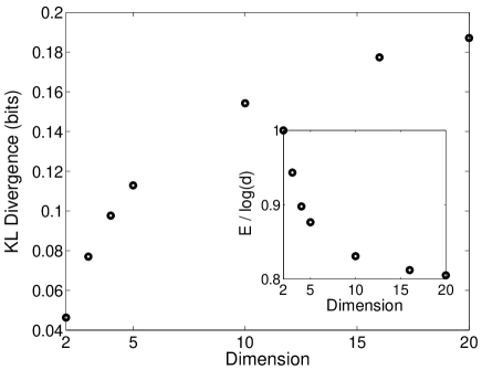
Figure 1: KL Divergence for Bell tests using two projective measurements under the mentioned assumptions. In the inset, it is shown the amount of entanglement, in terms of Entropy of Entanglement, for the optimal state, $|\Psi_{d}\rangle$.

Discussion: Figure 1 shows several interesting features. First of all, one can see that for an optimal $2\times d$ Bell test, there is no need for systems of very large dimension. Actually, the simplest CHSH scenario for the singlet state already constitutes a reasonably good test for ruling out local models. However, beyond this simple case, none of the optimal Bell tests requires a maximally entangled state. In all the studied situations, the Schmidt basis for the optimal state was the computational one. Assuming this is always the case, we can compute the conjectured optimal state for large $d$, say $d=1000$, finding that $E(\Psi_{d})\rightarrow\ln d\approx 0.69\log d$ bits.

It also follows from Fig. 1 that two measurements per site may not be optimal for large $d$. For instance, when $d=16$ the conjectured optimal $2\times 16$ test is worse than the $4\times 16$ test consisting of two independent realizations of the optimal $2\times 4$ Bell test for two copies of $|\Psi_{4}\rangle$. Indeed, it is always possible to interpret two independent realizations of this Bell test as a “new” $2^{2}\times 4^{2}$ Bell test for $|\Psi\rangle^{\otimes 2}$. Using that (i) the KL Divergence is additive, $D(\vec{q}\,^{2}||\vec{p}\,^{2})=2D(\vec{q}\,||\vec{p})$, and (ii) the closest local model to two independent realizations of the same Bell test corresponds to two independent realizations of the best local model for the single-copy case, the KL Divergence for this test is twice the initial one.

A priori, one would have expected the maximally entangled state to be the optimal state for any Bell test. A thorough numerical search of Bell tests for the maximally entangled state $|\Phi_{3}\rangle$ using more settings per site and general measurements has been performed. No improvement over the optimal $2\times 3$ case was obtained. Actually, it is remarkable that Bell tests with two projective measurements per site are so good for low dimensional systems. Therefore, all the previous numerical results show that beyond qubits and for the same amount of resources (system dimension and number and type of settings) the optimal state for a Bell test is not maximally entangled.

Conclusions: Non-local correlations constitute an information theoretic resource per se BLMPPR , that can be distributed by means of quantum states. It is known that there are nonlocal correlations that cannot be established by measuring quantum states PR . Moreover, the nonlocal correlations obtained from the maximally entangled state $|\Phi_{3}\rangle$ seem to be less robust against noise than those from $|\Psi^{mv}_{3}\rangle$ ADGL . Actually, the communication cost of simulating the nonlocal correlations for $|\Psi^{mv}_{3}\rangle$ seems to be higher than for $|\Phi_{3}\rangle$ Pironio . More recently, it has been shown that the so-called nonlocal machine PR ; BLMPPR is sufficient for the simulation of the correlations in a singlet state CGMP , but it fails for some nonmaximally entangled states of two qubits BGS . All these result suggest that, despite the fact that all pure entangled states contain nonlocal correlations Gisin , the relation between entanglement and nonlocality is subtler than firstly expected, since they may represent different information resources.

In this work, entangled states are analyzed as a tool for the construction of Bell tests. For all the studied scenarios and beyond the qubit case, the states needed for an optimal Bell test are not maximally entangled.

This work is supported by the ESF, an MCYT “Ramón y Cajal” grant, the Generalitat de Catalunya, the Swiss NCCR “Quantum Photonics” and OFES within the EU project RESQ (IST-2001-37559).

References

- (1) J. S. Bell, Physics 1, 195 (1964).
- (2) A. Aspect, P. Grangier and G. Roger, Phys. Rev. Lett. 47, 460 (1981); W. Tittel et al., ibid 81, 3563 (1998); G. Weihs et al., ibid 81, 5039 (1998); M. Rowe et al., Nature 409, 791 (2001).
- (3) A. Einstein, B. Podolsky and N. Rosen, Phys. Rev. 47, 777 (1935).
- (4) See for instance M. A. Nielsen and I. L. Chuang, Quantum Computation and Quantum Information, Cambridge University Press (2000).
- (5) C. H. Bennett, H. J. Bernstein, S. Popescu and B. Schumacher, Phys. Rev. A 53, 2046 (1996).
- (6) N. Gisin, Phys. Lett. A 154, 201 (1991).
- (7) S. Popescu, D. Rohrlich, Found. Phys. 24, 379 (1994).
- (8) A. Acín, N. Gisin, L. Masanes and V. Scarani, Int. J. Quant. Inf. 2, 23 (2004).
- (9) D. Mayers and A. Yao, Quant. Inf. Comp. 4, 273 (2004).
- (10) W. van Dam, R. Gill and P. Grünwald, quant-ph/0307125; to appear in IEEE Trans. Inf. Theory.
- (11) T. M. Cover and J. A. Thomas, Elements of Information Theory, Wiley Interscience, New York (2000).
- (12) A. Peres, Fortsch. Phys. 48, 531 (2000).
- (13) J. F. Clauser, M. A. Horne, A. Shimony, R. A. Holt, Phys. Rev. Lett. 23, 880 (1969).
- (14) D. Collins et al., Phys. Rev. Lett. 88, 040404 (2002).
- (15) D. Kaszlikowski et al., Phys. Rev. Lett. 85, 4418 (2000).
- (16) A. Acín, T. Durt, N. Gisin and J. I. Latorre, Phys. Rev. A 65, 052325 (2002).
- (17) J. Barrett et al., Phys. Rev. A 71, 022101 (2005).
- (18) S. Pironio, Phys. Rev. A 68, 062102 (2003).
- (19) N. J. Cerf, N. Gisin, S. Massar and S. Popescu, Phys. Rev. Lett. 94, 220403 (2005).
- (20) N. Brunner, N. Gisin and V. Scarani, New J. Phys. 7, 88 (2005).