Abstract:

This communication is an enquiry into the circumstances under which concurrence and phase entropy methods can give an answer to the question of quantum entanglement in the composite state when the photonic band gap is exhibited by the presence of photonic crystals in a three-level system. An analytic approach is proposed for any three-level system in the presence of photonic band gap. Using this analytic solution, we conclusively calculate the concurrence and phase entropy, focusing particularly on the entanglement phenomena. Specifically, we use concurrence as a measure of entanglement for dipole emitters situated in the thin slab region between two semi-infinite one-dimensionally periodic photonic crystals, a situation reminiscent of planar cavity laser structures. One feature of the regime considered here is that closed-form evaluation of the time evolution may be carried out in the presence of the detuning and the photonic band gap, which provides insight into the difference in the nature of the concurrence function for atom-field coupling, mode frequency and different cavity parameters. We demonstrate how fluctuations in the phase and number entropies effected by the presence of the photonic-band-gap. The outcomes are illustrated with numerical simulations applied to GaAs. Finally, we relate the obtained results to instances of any three-level system for which the entanglement cost can be calculated. Potential experimental observations in solid-state systems are discussed and found to be promising.

PACS numbers: 42.50.Dv, 03.65.Ud, 03.67.Mn

1 Introduction

A structure in which the dielectric constant varies periodically is called a photonic crystal. One of the most interesting properties of a photonic crystal is the existence of a photonic band gap [1, 2]. Radiation with a frequency that lies within the band gap cannot propagate in the photonic crystal structure. Photonic crystals are usually viewed as an optical analog of semiconductors that modify the properties of light similar to a microscopic atomic lattice that creates a semiconductor band-gap for electrons [1, 3, 4]. Photonic band gap crystals offer unique ways to tailor light and the propagation of electromagnetic waves and have caused growing interest in recent years because it offers the possibility of controlling and manipulating light within a given frequency range through photonic band gap [1, 3]. Photonic band-gap materials have attracted much attention in recent years for theoretical and practical importance in fundamental science and application [1, 4]. The atom-photon interaction in photonic band gap materials [4] has been found to exhibit many interesting new phenomena such as photon-atom bound states [5], spectral splitting [6], quantum interference dark line effect [7], phase control of spontaneous emission [8], transparency near band edge [9], and single-atom switching [10].

In a parallel development, considerable work was done recently on entanglement properties [11]. The detection of entanglement is one of the fundamental problems in quantum information theory. From a theoretical point of view one can try to answer the question whether a given entirely known state is entangled or not, but despite a lot of progress in the last years [11,12], no general solution of this problem is known. In experiments, one aims at detecting entanglement without knowing the state completely. Bell inequalities [14] and entanglement witnesses [15] are the main tools to tackle this task. Interestingly, the concurrence of the ground state which is related to the entanglement of formation, has been shown to be strongly affected at the critical point [16]. More precisely, in the one-dimension, it has been shown that the derivative of the concurrence with respect to the coupling constant diverges at the transition point, although the concurrence itself is not maximum. These pioneering results raise the question of the universality of these behaviors. Actually, the lack of exact solutions especially in higher dimensions implies a numerical treatment which often restrict the study to a small number of degrees of freedom.

Heisenberg’s uncertainty relations had tremendous impact in the field of quantum optics particularly in the context of the construction of coherent states and also for different physical systems as well as the reconstruction of quantum states. The minimization problem of finding the number-phase uncertainty state has been considered and minimum uncertainty state relations between number and phase uncertainty are presented [17]. Many authors argued that [12], the Heisenberg inequality is too weak for practical purposes, which led them to the establishment of information theoretic uncertainty relations.

Our aim of the present paper is to consider the dynamics of a system of three-level atoms with dipole interaction in presence of the photonic band gap and study the concurrence and the entropic uncertainty relation for number and phase. With applying some approximations, one can deal with the quantization of the electromagnetic field modes of a homogeneous, but anisotropic medium which can then be made to form one of the sandwich layers in the slab structure under consideration involving two semi-infinite periodic photonic crystals. With the electromagnetic modes quantized, one can evaluate the entanglement degree, and explore its variations with the controllable parameters of the system. To reach our goal we have to find an exact analytic solution of the time dependent Schrödinger equation of the system. We show that a reasonable amount of entanglement can be achieved in a system of three-level atoms with dipole interaction in presence of the photonic band gap and essentially we establish deeper connections between entropic uncertainty relations and entanglement.

The organization of this paper is as follows: in section 2, we give an overview of effective medium approach and dispersions, followed by subsection 2.1 where we introduce our Hamiltonian model and give exact analytic solution for the Schrödinger equation in the frame of the dressed state formalism. In section 3, we employ the analytical results obtained in section 2 to investigate the properties of the entanglement degree due to the concurrence, and classify the behavior in several parameter regimes assuming that the electromagnetic field is in a coherent state in subsection 3.1. In section 4, we essentially establish deeper connections between entropic uncertainty relations and entanglement. Numerical results for the phase entropy are discussed in the subsection 4.1 for two different cases; one is the resonant and the other is the off-resonant case. The prospects for experimental observation of our predictions are analyzed in section 5. Finally, a summary of the main points of this work ends the paper and a few avenues for further investigations are indicated in section 6.

2 Effective medium approach

The effective-medium approach can be applied to situations in which all three regions of the structure possess frequency-dependent dielectric functions. In fact, the rapid pace of the technological progress in solid-state quantum computing gives one a hope that the specific prescriptions towards building robust qubits and their assemblies discussed in this work can be implemented in future devices. In this regard, very promising fields where the concept of nonlinear localized modes may find practical applications is the quantum computation of photonic band gap materials, periodic dielectric structures that produce many of the same phenomena for photons as the crystalline atomic potential does for electrons [4,18]. Nonlinear photonic crystals (or photonic crystals with embedded nonlinear impurities) create an ideal environment for the generation and observation of nonlinear localized photonic modes. Much theoretical work has been done on the properties of finite one dimensional photonic band gap (PBG) crystals [4], including recent calculations of the thermal emissivity of such one-dimensional structures [19]. The strong angular dependence of the gap effect with a one-dimensional structure has motivated successful experimental work with three-dimensional structures [20]. In particular, the existence of such modes for the frequencies in the photonic band gaps has been predicted [21] for $2D$ and $3D$ photonic crystals with Kerr nonlinearity. Nonlinear localized modes can also be excited at nonlinear interfaces with quadratic nonlinearity [22], or along dielectric waveguide structures possessing a nonlinear Kerr-type response [23].

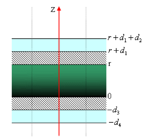
Figure 1: A schematic representation of the dielectric slab between two photonic crystals occupying the regions $z<0$ and $z>r$.

The system that we consider here consists of a dielectric cavity occupying the region $0<z<r$ and the photonic crystals occupy the regions $z>r$ and $z<0$. For long wavelength fields and in the effective medium approach, the photonic crystal has the optical characteristic of a uniaxial medium [3]. Moreover we shall specialize to uniaxial media, so that our system has only two principal axes with the $z-$axis as the optical axis. In this case, the components of the dielectric tensor appropriate to the photonic crystals can be written as

$$\epsilon=\left(\begin{array}[]{c}\epsilon\\ 0\\ 0\end{array}\begin{array}[]{c}0\\ \epsilon\\ 0\end{array}\begin{array}[]{c}0\\ 0\\ \epsilon_{z}\end{array}\right),$$ (1)

where, $\epsilon=\epsilon_{0}\epsilon^{||},$ $\epsilon_{z}=\epsilon_{0}\epsilon_{z}.$ The dielectric tensor components for the two semi-infinite crystals can be written in the following forms $\epsilon_{1}^{||}=(\eta_{1}d_{1}+\eta_{2}d_{2})/d_{12},\qquad\epsilon_{z1}=\eta_{1}\eta_{2}d_{12}/(\eta_{1}d_{2}+\eta_{2}d_{1}),$ and $\epsilon_{2}^{||}=(\eta_{3}d_{3}+\eta_{4}d_{4})/d_{34},\qquad\epsilon_{z2}=\eta_{3}\eta_{4}d_{34}/(\eta_{3}d_{4}+\eta_{4}d_{3}),$ where the $d_{ij}=d_{i}+d_{j},$ the subscripts 1 and 2 on $\epsilon_{i}^{||}$ and $\epsilon_{zi}$ refer to the first and second photonic crystal. The dielectric functions $\eta_{1}$ and $\eta_{2},$ one or both of which may be frequency dependent. The photonic crystals are treated using the effective medium approach, which pertains to any layer structure formed by alternate periodic stacking of two types of layers of locally isotropic materials of thicknesses d₁ and $d_{2}$ (see figure 1).

In this paper we are concerned with the interface polaritons which are characterized by imaginary wave vectors normal to the interfaces such that the waves are decaying with distance from the interfaces at $z=0$ and $z=r$ into the outer regions and are hyperbolic in the slab [3, 23, 24]. To see the salient features of the effective medium description we shall ignore retardation effects, which amounts to ignoring throughout ($\omega/c$) terms. In this case dispersion relation for the surface polaritons takes the form

$$k_{s}r=\arctan h\left(-\frac{k_{s}}{\epsilon_{s}}\times\frac{(k_{1}/\epsilon_{1}^{||})+(k_{2}/\epsilon_{2}^{||})}{(k_{s}/\epsilon_{s})+(k_{1}k_{2}/\epsilon_{1}^{||}\epsilon_{2}^{||})}\right).$$ (2)

The dispersion relations obtained from the Maxwell wave equation of this system lead to two distinct equations [25] $k_{s}^{2}=k_{||}^{2}-\omega^{2}\epsilon_{s}/c^{2},\quad k_{i}^{2}=\epsilon_{i}^{||}k_{||}^{2}/\epsilon_{zi}-\omega^{2}\epsilon_{i}^{||}/c^{2},$ where s refers to the slab cavity.

It is important to note that infinite and semi-infinite photonic crystals have the same band structure [26]. The only difference is the existence of surface modes in the case of semi-infinite structure. The main feature of all 1D photonic crystals is that although forbidden gaps exist for most given values of the tangential component of the wave vector ($k$), there is not an absolute nor complete photonic band gap if all possible values of the tangential component of the wave vector are considered [4]. Having determined the modes we can now quantize the fields associated with these modes using the usual quantization procedure [3] the single-mode quantized field takes the form

$$E(\hat{x},t)=E_{0}\hat{a}(\hat{k}_{||})\exp[i(\hat{k}_{||}.\hat{x}-\omega t)]+H.C.,$$ (3)

where $E_{0}$ is the strength of the electric field, $\hat{k}_{||}$ is the wave vector, $\hat{x}$ is the position operator and $\hat{a}$ the annihilation operator.

2.1 The model and methods of solution

Accurate potentials are of course required for a quantitatively correct prediction of the behavior and properties of real quantum systems. However, even qualitative conclusions drawn from simulations employing inaccurate or invalidated potentials can be problematic. The most appropriate form of the potential depends largely upon the properties of interest to the simulators. Now we consider the interaction of the abovementioned modes with a three-level atom in three different configurations, namely, $V-,$ Lambda- and cascade-type. The transition in the 3-level atom is characterized by the dipole matrix element $\lambda_{ij}.$ The operator $\hat{S}_{ii}$ describes the atomic population of level $|i\rangle_{A}$ with energy $\omega_{j},(j=a,b,c)$ and the operator $\hat{S}_{ij},(i\neq j)$ describes the transition from level $|i\rangle_{A}$ to level $|j\rangle_{A}$.

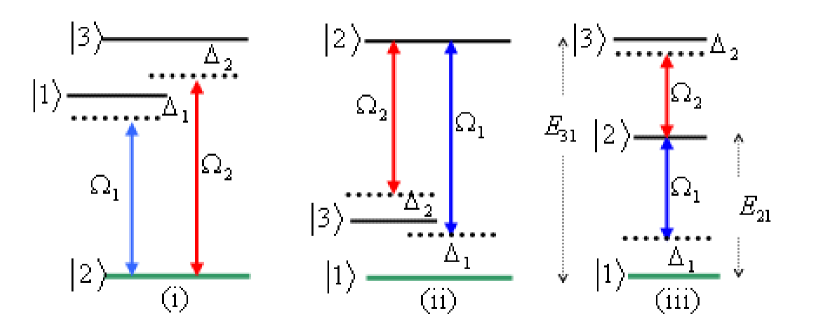
Figure 2: The V-type, $\Lambda$-type and $\Xi$-type three-level atom interacting with a bimodal field. The levels $|1\rangle_{A}$, $|2\rangle_{A}$, and $|3\rangle_{A}$, have the energy values $\hbar\omega_{1},\hbar\omega_{2}$ and $\hbar\omega_{3}$, respectively. The transitions $|1\rangle_{A}\longrightarrow|2\rangle_{A}$ , and $|2\rangle_{A}\longrightarrow|3\rangle_{A}$, are coupled to two intra-cavity different modes $\hat{a}_{1}$ and $\hat{a}_{2}$ with eigenfrequencies $\Omega_{1}$ and $\Omega_{2}$. The detunings of the levels $|1\rangle_{A},|2\rangle_{A}$, and $|2\rangle_{A},|3\rangle_{A}$, are $\Delta_{1}=\omega_{1}-\omega_{2}-\Omega_{1}$ and $\Delta_{2}=\omega_{3}-\omega_{2}-\Omega_{2}$, for V-type, and $\Xi$-type, while $\Delta_{1}=\omega_{2}-\omega_{1}-\Omega_{1}$ and $\Delta_{2}=\omega_{2}-\omega_{3}-\Omega_{2}$ for $\Lambda$-type.

The total Hamiltonian of this system is $\hat{H}=\hat{H}_{0}+\hat{H}_{int}$. The $3$ eigenstates, $\left|\xi_{i}\right\rangle$ and corresponding eigenenergies, $\alpha_{i}$ are assumed to be known. The total wave-function may be expanded in terms of the known eigenstates, namely

$$\left|\Psi(t)\right\rangle=A_{1}(t)\left|\xi_{1}\right\rangle+A_{2}(t)\left|\xi_{2}\right\rangle+A_{3}(t)\left|\xi_{3}\right\rangle.$$ (4)

With atomic units, using Schrödinger equation, we obtain the coupled equations for our three-level system, namely

$$i\frac{\partial A_{j}(t)}{\partial t}=r_{j}A_{j}(t)+\sum\limits_{k=1}^{3}H_{jk}A_{k}(t),$$ (5)

where $\hat{H}_{0}\left|\xi_{i}\right\rangle=r_{i}\left|\xi_{i}\right\rangle$ and $H_{jk}=\left\langle\xi_{j}\right|\hat{H}_{int}\left|\xi_{k}\right\rangle.$ These equations are exact for any three-level atom. In the interaction picture, let us consider a three-level system described, in an appropriate rotating frame, by the Hamiltonian

$$\hat{H}_{int}=\Delta_{1}\hat{S}_{11}+\Delta_{2}\hat{S}_{33}+\lambda_{21}\hat{R}_{1}\hat{S}_{21}+\lambda_{32}\hat{R}_{2}\hat{S}_{32}+\lambda_{21}^{\ast}\hat{R}_{1}^{\dagger}\hat{S}_{12}+\lambda_{32}^{\ast}\hat{R}_{2}^{\dagger}\hat{S}_{23}.$$ (6)

The atom-field couplings $\lambda_{ij}$ are given by $\lambda_{ij}=Y\mu_{ij}.E,$where $E$     is the quantized electric field given by equation (3) and $\mu_{ij}$ is the matrix dipole moment coupling between the state $i$ and $j$. The $Y$ factor accounts for local field effects and is given by $Y=3\epsilon_{s}(\omega)/(2\epsilon_{s}(\omega)+1),$ where $\epsilon_{s}(\omega)$ is given in equation (1). It is easy to write $\lambda_{ij}$ in the following form

$$\lambda_{ij}=\frac{3\epsilon_{s}(\omega)}{2\epsilon_{s}(\omega)+1}.\frac{\left(\omega/\omega_{T}\right)^{2}-\left(\omega_{L}/\omega_{T}\right)^{2}}{\left(\omega/\omega_{T}\right)^{2}-\eta^{2}},$$ (7)

where $\eta^{2}=[$ $2\epsilon_{s}(\omega)\left(\omega_{L}/\omega_{T}\right)^{2}+1]/[2\epsilon_{s}(\omega)+1]$. The transitions between the three levels may occur in three different configurations depending upon the relationship between the energies $E_{1},E_{2}$ and $E_{3}$ of levels $1,2$ and $3$. The possible configurations are [27] (i) the $V$-type corresponding to $E_{2}<E_{1}<E_{3}$, (ii) the $\Lambda-$type or Raman configuration corresponding to $E_{1}<E_{3}<E_{2}$ and (iii) the $\Xi-$type or ladder-type corresponding $E_{1}<E_{2}<E_{3}$. Each of the two pairs of levels can be coupled by only one-mode or two-mode. The field operators in the abovementioned three types are (i) $F_{1}=\hat{a}^{\dagger},F_{2}=\hat{b}$ for $V$-type, (ii) $F_{1}=\hat{a},F_{2}=\hat{b}^{\dagger}$ for $\Lambda$ -type and (iii) $F_{1}=\hat{a},F_{2}=\hat{b}$ for $\Xi$-type with $\hat{a}=\hat{b}$ if both pairs of levels are coupled by the same mode.

In order to solve equations (5), we assume that [27]

$$G(t)=A(t)+xB(t)+yC(t),$$ (8)

which means that

$$i\frac{dG(t)}{dt}=\left(r_{1}+v_{1}^{\ast}y\right)\left\{A(t)+\frac{r_{2}x+v_{2}^{\ast}y}{r_{1}+v_{1}^{\ast}y}B(t)+\frac{v_{2}x+r_{3}y}{r_{1}+v_{1}^{\ast}y}C(t)\right\},$$ (9)

where $v_{1}$ and $v_{2}$ are given using equations (5) and (6). We seek $G(t)$ such that $i\overset{.}{G}(t)=zG(t)$. This hold if

$$y=\frac{v_{2}x+r_{3}y}{r_{1}+v_{1}^{\ast}y},\quad x=\frac{r_{2}x+v_{2}^{\ast}y}{r_{1}+v_{1}^{\ast}y},\quad z=r_{1}+v_{1}^{\ast}y.$$

After some algebra this leads to a cubic equation which has three eigenvalues $x_{i}(y_{i})$ which determine the $z_{i}$. There are also three corresponding eigenfunctions $G_{j}(t)=G_{j}(0)\exp(-iz_{j}t)$, where

$$G_{j}(t)=M_{j1}A(t)+M_{j2}B(t)+M_{j3}C(t),$$ (10)

where

$$M_{ji}=\left(\begin{array}[]{c}1\\ 1\\ 1\end{array}\begin{array}[]{c}x_{1}\\ x_{2}\\ x_{3}\end{array}\begin{array}[]{c}y_{1}\\ y_{2}\\ y_{3}\end{array}\right).$$ (11)

Now, we express the unperturbed state amplitude $A(t),B(t)$ and $C(t)$ in terms of the dressed state amplitude $R_{j}$

$$F_{i}(t)=\sum\limits_{j=1}^{3}M_{ij}^{-1}G_{j}(t)=\sum\limits_{j=1}^{3}M_{ij}^{-1}G_{j}(0)\exp(-iz_{j}t),$$ (12)

$F_{1,2,3}(t)=A,B,C.$ Using the above equations, we can write

$$A(t) = \frac{1}{D}\left[(x_{2}y_{3}-y_{2}x_{3})e^{-iz_{1}t}+(x_{3}y_{1}-y_{3}x_{1})e^{-iz_{2}t}+(x_{1}y_{2}-y_{1}x_{2})e^{-iz_{3}t}\right],$$

$$B(t) = \frac{1}{D}\left[(y_{2}-y_{3})e^{-iz_{1}t}+(y_{3}-y_{1})e^{-iz_{2}t}+(y_{1}-y_{2})e^{-iz_{3}t}\right],$$ (13)

$$C(t) = \frac{1}{D}\left[(x_{2}-x_{3})e^{-iz_{1}t}-(x_{3}-x_{1})e^{-iz_{2}t}-(x_{1}-x_{2})e^{-iz_{3}t}\right],$$

where $D=\det(M)=x_{1}y_{2}+x_{2}y_{3}+x_{3}y_{1}-x_{1}y_{3}-x_{2}y_{1}-x_{3}y_{2}.$ We have thus completely determined the dynamics of a three-level system in the presence of photonic crystal.

The picture in this case is of the three-level system in the presence of photonic band gap and the detuning, rather than the usual picture of the three-level Jaynes-Cummings model (JCM) system. The important point to note here is that, using the above analytic approach, any three-level Hamiltonian is likewise exactly solvable, with precisely similar eigenvectors and eigenvalues that are obtained directly using equations (4) and (6). In Ref. [28] an analytic approach is proposed for three-level systems, based on the Riccati nonlinear differential equation. However, the solution obtained is valid only in certain situations. On the other hand, our analytic approach removed the restriction that considered in the previous work and this solution is valid for any three-level system.

Next, we discuss a frequently encountered phenomena of particular interest in which we define the entanglement measure of the present system.

3 Concurrence

Quantum entanglement has recently been attracted much attention as a potential resource for communication and information processing [29] . Entanglement is usually arise from quantum correlations between separated subsystems which can not be created by local actions on each subsystem. The concept of concurrence originates from the seminal work of Hill and Wootters [16] where the exact expression of the entanglement of formation of a system of two qubits was derived. They showed that the entanglement of formation, an entropic entanglement monotone, is a convex monotonic increasing function of the concurrence.

It has been shown that the concurrence of a mixed two-qubit state, $C(\rho_{AB})$, can be expressed in terms of the minimum average pure-state concurrence, $C\left(\left|\psi_{AB}\right\rangle\right)$, where the minimum is taken over all possible ensemble decompositions of $\rho_{AB}.$ So that, the concurrence is defined of a mixed state $\rho$ for $2\times 2$ quantum systems, in the following form [16]

$$C(\rho)=\max\left(\sigma_{1}-\sigma_{2}-\sigma_{3}-\sigma_{4}\right),$$ (14)

where the $\sigma_{i}$ are the square roots of the eigenvalues of the product matrix $Q$, the singular values (by convention sorted in descending fashion), all of which are non-negative real quantities

$$Q=\sqrt{\rho}^{T}\sigma_{y}\otimes\sigma_{y}\sqrt{\rho},$$ (15)

$\sigma_{y}$ is the well-known Pauli matrix, and $\sqrt{\rho}$ is any matrix satisfying $\sqrt{\rho}=\sqrt{\rho}^{\dagger}.$ The importance of this measure follows from the direct connection between concurrence and entanglement of formation $E_{f}$

$$E_{f}\left(\rho\right)=-\mu_{+}\ln\mu_{+}-\mu_{-}\ln\mu_{-},$$ (16)

where

$$\mu_{\pm}=\frac{1}{2}\left(1\pm\sqrt{1-C(\rho)^{2}}\right).$$ (17)

One can prove that $\rho$ is separable if and only if the concurrence is zero.

Let us now turn our attention to the definition of the concurrence of a pure state [30] on a $(N\times K)-$dimensional Hilbert space $\Re=\Re_{N}\otimes\Re_{K}.$ The flip operator $\mathit{F}$  acting on an arbitrary Hermitian operator $A$ on $\Re$ can be written as

$$F(A):=A+(trA)\Pi-(tr_{N}A)\otimes\Pi_{K}-\Pi_{N}\otimes(tr_{K}A),$$ (18)

where $tr_{N}$ and $tr_{k}$ the partail traces over $\Re_{N}$ and $\Re_{K},$ respectively. We denote by $\Pi_{N}$ and $\Pi_{K}$ the identity on $\Re_{N}$ and $\Re_{K},$ respectively. The expectation value $\left\langle\psi\right|F(\rho_{\psi})\left|\psi\right\rangle,$ where $\rho_{\psi}=\left|\psi\right\rangle\left\langle\psi\right|$, is non-negative for all pure states and equals zero if and only if $\left|\psi\right\rangle$ is a product state. This allows to define the concurrence of any arbitrary bipartite pure state as [30]

$$C\left(\left|\psi\right\rangle\right) = \sqrt{\left\langle\psi\right|F(\rho_{\psi})\left|\psi\right\rangle}$$ (19)

$$= \sqrt{2\left(\left\langle\psi|\psi\right\rangle^{2}-tr(\rho_{N}^{2})\right)},$$

where $\rho_{N}=tr_{K}\left(\rho_{\psi}\right)$ is the reduced density operator of dimension N. For a normalized state, $\left\langle\psi|\psi\right\rangle=1,$ it interpolates monotonously between zero for product states and $\sqrt{\frac{2(N-1)}{N}}$ for maximally entangled states.

To investigate the concurrence for the system under consideration, we have to evaluate the reduce atomic density matrix $\rho_{{}_{A}}=tr_{{}_{F}}\rho(t),$ which can be written as

$$\rho_{{}_{A}}=\sum_{i=1,2,3}\rho_{{}_{ii}}\left|i\right\rangle\left\langle i\right|+\sum_{i,j=1,2,3,i\neq j}\rho_{{}_{ij}}\left|i\right\rangle\left\langle j\right|,$$ (20)

where $\rho_{ij}(t)=\langle i|\rho_{{}_{A}}(t)|j\rangle,\quad i,j=1,2$ and $3.$ Using equations (19) and (20), we can write the concurrence in the following form

$$C\left(\left|\psi\right\rangle\right)=\sqrt{2\sum_{i,j=1,2,3,i\neq j}\left(\rho_{{}_{ii}}\rho_{{}_{jj}}-\rho_{{}_{ij}}\rho_{{}_{ji}}\right)}.$$ (21)

Although the concurrence and therefore the results we obtain are not restricted to the standard one-mode three-level system, we will use that language throughout most of the paper.

Having specified the various photonic crystal and field amplitude parameters, we will present in the following subsection the results of our numerical analysis of the concurrence.

3.1 Numerical results

For applications in real systems, we consider the dipole emitters with frequencies in the reststrahl band of  GaAs. In this subsection we will discuss the time dependence of the concurrence, which considered as an entanglement measure. We will consider the commonly used state as initial condition for the cavity field: the coherent state, which may be applicable in different situations. As might be expected, the behavior of the three-level system changes dramatically depending on the initial field state. Throughout this subsection the quantity to be examined is the concurrence $C\left(\left|\psi\right\rangle\right).$

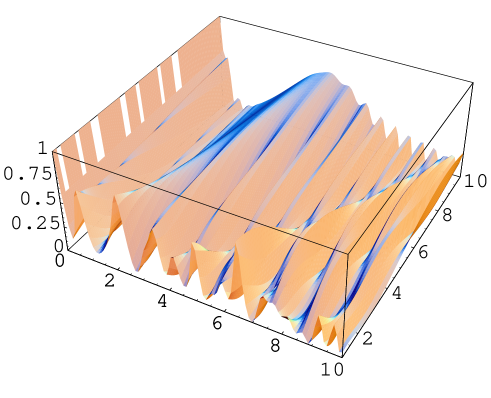
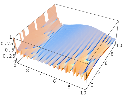
Figure 3: The evolution of the concurrence $C\left(\left|\psi\right\rangle\right)$ as a function of the scaled time $\lambda_{1}t$ and the mean photon number $\bar{n}$. The parameters are $\epsilon_{0}=10.89,$ $\eta=1.085,$ $\omega/\omega_{T}=2,$ $\omega_{0}/\omega_{T}=1,$ $\hslash\omega_{L}=36.29$meV, $\hslash\omega_{T}=33.25$meV, $d_{1}=500$ Å, $d_{2}=300$Å, $\epsilon_{1}=9,$ $\epsilon_{2}=1.3,$ $d_{3}=500$Å, $d_{4}=400$Å, $\epsilon_{3}=10,$ $\epsilon_{4}=1.5$ and $L=1.5d$, and different values of the detuning parameter, where $\Delta=0$ for Fig. 3a and $\Delta=5\lambda_{1}$ for Fig 3b.

In figure 3, we present the oscillatory behavior of the concurrence $C\left(\left|\psi\right\rangle\right)$ against the scaled time $\lambda_{1}t$ and the mean photon number $\overline{n}$ for different values of the detuning parameter, where $\Delta=0$ for Fig. 3a and $\Delta=5\lambda_{1}$ for Fig 3b. We consider a specific system in which the cavity is taken as GaAs with $\epsilon_{0}=10.89,$ $\eta=1.085,$ $\omega/\omega_{T}=2,$ $\omega_{0}/\omega_{T}=1,$ $\hslash\omega_{L}=36.29$meV, $\hslash\omega_{T}=33.25$meV. The photonic crystals parameters are given by the arbitrary set, $d_{1}=500$Å, $d_{2}=300$Å, $\epsilon_{1}=9,$ $\epsilon_{2}=1.3,$ $d_{3}=500$Å, $d_{4}=400$Å, $\epsilon_{3}=10,$ $\epsilon_{4}=1.5$ and $L=1.5d.$ The general behavior due to the coherent state of the field does not contain any surprises it is quite broad, corresponding to the standard quantum limit. The value of concurrence at the first maximum is 1, which is quit remarkable, see figure 3a. After the time goes on, we see that the maximum value of the concurrence decreases with small amplitude of the oscillations. As the mean photon number increased, the number of oscillations decreased.

The effect of the parameter which describes the mismatch between the atomic frequency and the mean frequency of the cavity mode has been considered in figure 3b. We set the other parameters as the same as in figure 3a, and $\Delta=5\lambda_{1}$. As $\Delta$ is increased the behavior of the three-level system becomes increasingly erratic. Shorter revival times cause successive revivals to overlap and interfere so that the time evolution appears irregular. The detuning parameter at which irregularity emerges is closely tied to the mean-photon number: the higher the mean-photon number, the smaller the detuning needed to produce irregular behavior. Larger detuning also results in decreased revival amplitude due to the larger number of frequencies in the sum, which causes the rephasing to be less complete. However, a signature of the revivals persists as a return to the bare Rabi frequency even at mean-photon number high enough that the behavior looks random and the revival amplitude is essentially washed out. From our further calculations (which are not presented here), we point out that as we increase the value of the detuning one can see that the revival time is also prolonged, however the period of fluctuations is decreasing. Detuning affects the revival time by elongating it and the maximum value of the entanglement degree becomes smaller and smaller. Similar to the case of a two-level atom, detuning shifted the atomic occupation probability around which it oscillates upward meaning that the energy is stored in the atomic system.

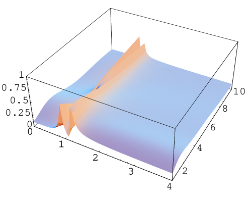
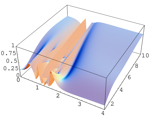
Figure 4: The evolution of the concurrence $C\left(\left|\psi\right\rangle\right)$ as a function of the mode-frequency $\omega/\omega_{T}$ and the mean photon number $\bar{n}$ for different values of the scaled time, where $\lambda_{1}t=\pi/2$ for Fig. 4a and $\lambda_{1}t=3\pi/2$ for Fig 4b.

Now we will turn our attention to the effect on the concurrence of the mode frequency $\omega/\omega_{T}$. In particular, we consider $\epsilon_{0}=10.89,$ $\eta=1.085,$ $\omega_{0}/\omega_{T}=1$ and for different values of the scaled time, where $\lambda_{1}t=\pi/2$ for Fig. 4a and $\lambda_{1}t=3\pi/2$ for Fig 4b. Our particular observation is the maximum entanglement occurs near the band edges, which corresponds to $\omega=1.085\omega_{T}$. Near the band edges the wave vector parallel to the interface reaches its maximum value, and this corresponds to the first two relatively small peaks around the point $1.085$. In the gap region or the reststrahl region of the $GaAs$ system no electromagnetic fields can propagate and coupling is therefore suppressed. The extra peaks around the point $1.085$ are attributed to local field effects and can be understood from looking at equation (7) where $\lambda_{ij}$ has a pole at $\eta=\omega/\omega_{T}.$ One has to bear in mind that the above calculation did not take into explicit account the spatial dependence of the coupling parameters. Therefore, a more careful calculation would have to take into account the nonstationary property of the present system. The above model calculations suggest that physical parameters such as mode frequency, mode-atom coupling and cavity dielectric have important effects on the entanglement. One can see that the oscillations collapse after few Rabi periods and after an interval of time in which the concurrence is constant, the oscillations reappear again. This revival then collapses and a new revival begins.

This behavior highlights once again the role of the functional form of the modified Rabi frequencies in controlling the time evolution of the concurrence. Rabi frequencies which obtained in the present model are similar to that obtained from the standard three-level model but involving a frequency-dependent dielectric function. An important point to keep in mind when comparing the results presented here with results from the usual three-level system in the absence of the photonic band gap is that: they are give a different feature relative to the entanglement. This raises an interesting question: can one use the present system in building quantum logic gates? Calculations and detailed discussion of this issue will be presented in a forthcoming paper.

4 Phase entropy

One of the most striking features of quantum mechanics is the property that certain observable cannot simultaneously be assigned arbitrarily precise values. This property does not compromise claims of completeness for the theory, since it may consistently be asserted that such observable cannot simultaneously be measured to an arbitrary accuracy [17]. The Shannon entropies associated with the photon number distribution $P_{m}$ and phase probability distribution $P(\theta,t),$

$$P_{m} = \langle m|\rho(t)|m\rangle,$$

$$P(\theta,t) = \langle\theta|\rho(t)|\theta\rangle,$$ (22)

where $|m\rangle$ is the Fock state and $|\theta\rangle$ is the phase state, are given respectively by [17]

$$R_{N} = -\sum\limits_{m=0}^{\infty}P_{m}\ln P_{m},$$

$$R_{\psi} = -\int\limits_{2\pi}\left(P(\theta,t)\ln P(\theta,t)\right)d\theta.$$ (23)

The entropic uncertainty relations for the number and phase distribution determine the lower bound on the sum of the Shannon entropies $R_{N}$ and $R_{\psi}:$

$$R_{N}+R_{\psi}\geq\ln(2\pi).$$ (24)

This equality is satisfied by a Fock state for which $R_{N}=0$ and $R_{\psi}=\ln(2\pi).$ Other physical states give an entropic sum greater than $\ln(2\pi).$ Specifically, for a coherent state we find that the sum is $\ln(e\pi)$ for the mean photon number greater than one, i.e.

$$R_{N}+R_{\psi}\geq\ln(e\pi).$$ (25)

The lower bound for the position-momentum entropic uncertainty relation is also given by right-hand side of this equation i.e $\ln(e\pi).$

The single-mode of the Pegg-Barnett phase formalism which of interest in the field of quantum optics can be constructed from the single-mode phases [31] to take the form

$$P(\theta,t)=\lim_{s\rightarrow\infty}\biggl{(}\frac{s+1}{2\pi}\biggr{)}\langle\theta_{m}|\rho(t)|\theta_{m}\rangle,$$ (26)

$|\theta_{m}\rangle$ is a phase state of the mode,

$$|\theta_{m}\rangle=\frac{1}{\sqrt{(s+1)}}\sum_{n=0}^{s}e^{in\theta_{m}}|n\rangle,$$ (27)

where $\theta_{m}=\theta_{\circ}+\frac{2\pi m}{s+1},$ and $m=0,1,...s,$ and $\theta_{\circ}$ arbitrary. Equation (26) defines a particular basis set of $(s+1)$ mutually orthogonal phase states.

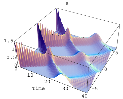
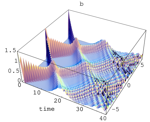
Figure 5: $P(\theta,t)$ against $\theta$ and the scaled time $\lambda_{1}t$. The parameters are $\epsilon_{0}=10.89,$ $\eta=1.085,$ $\omega/\omega_{T}=2,$ $\omega_{0}/\omega_{T}=1,$ $\hslash\omega_{L}=36.29$meV, $\hslash\omega_{T}=33.25$meV, $d_{1}=500$Å, $d_{2}=300$Å, $\epsilon_{1}=9,$ $\epsilon_{2}=1.3,$ $d_{3}=500$Å, $d_{4}=400$Å, $\epsilon_{3}=10,$ $\epsilon_{4}=1.5$ and $L=1.5d$, where (a) $\Delta=0$ and (b) $\Delta=5\lambda_{1}.$

Using the standard procedure [31], the phase probability distribution, the expectation value and the variance of the Hermitian phase operator may be obtained for the field. Since the coherent field at $t=0$ belongs to a class of partial phase states, we have chosen the reference phase $\theta_{0}$ as $\theta_{0}=\beta-\frac{\pi s}{s+1},$ and introduced the new phase labels $\zeta=m-\frac{1}{2}s$ where $m=0,1,2,...,s.$ Then as $s$ tends to infinity the summation may be transformed into an integral after replacing $\frac{2\pi\zeta}{s+1}$ by $\theta,$ and $\frac{2\pi}{s+1}$ by $d\theta.$ This leads to continuous phase probability distribution, where

$$P(\theta,t)=\frac{1}{2\pi}\left(1+2\sum\limits_{n>m}^{\infty}\left\{A_{n,m}(t)\cos[\theta(n-m)]+B_{n,m}(t)\sin[\theta(n-m)]\right\}\right),$$ (28)

where $A_{n,m}(t)$ and $B_{n,m}(t)$ are given by

$$A_{n,m}(t) = {Re}\left\{A_{n}(t)A_{m}^{\ast}(t)+B_{n}(t)B_{m}^{\ast}(t)+C_{n}(t)C_{m}^{\ast}(t)\right\},$$

$$B_{n,m}(t) = {Im}\left\{A_{n}(t)A_{m}^{\ast}(t)+B_{n}(t)B_{m}^{\ast}(t)+C_{n}(t)C_{m}^{\ast}(t)\right\}.$$ (29)

The phase probability distribution is normalized according to $\int_{-\pi}^{\pi}P(\theta,t)d\theta=1.$

4.1 Numerical results

In what follows we shall display some general arguments based on the equality sign in the Heisenberg uncertainty relations that to demonstrate the phase entropy of a general three-level system in the presence of photonic band gab when the initial state of the field is assumed to be in a coherent state.

In figure 5a, we have plotted the phase probability distribution $P(\theta,t)$ as a function of the scaled time $\lambda_{1}t$ and $\theta$ taking into consideration the presence of the photonic band gap. For example at time $\lambda_{1}t=0$ we realize that the phase distribution $P(\theta,t)$ starts with a single-peaked structure at $\theta=0$ corresponding to the initial coherent state. Then as the time develops the peak splits into two peaks moving into two opposite directions.

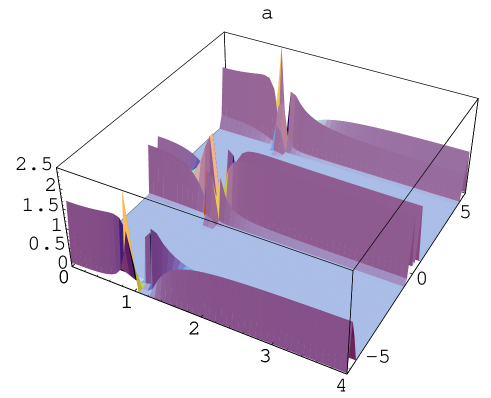
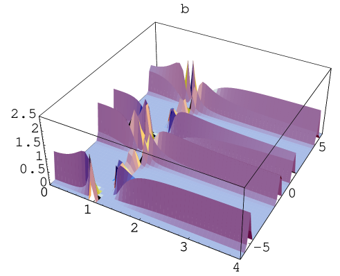
Figure 6: $P(\theta,t)$ against the mode-frequency $\omega/\omega_{T}$ and $\theta$. The parameters are the same as in figure 5, but (a) $\lambda_{1}t=\pi/2$ and (b) $\lambda_{1}t=3\pi/2.$

However the amplitudes of the split peaks fluctuate in time giving a top like shape until the two peaks reach the values $\theta=\pm\pi$ at middle of the revival time but in this range the amplitudes of the peaks do not show any fluctuations. The picture changes greatly as time develops further (say $\lambda_{1}t>40$) where we find that the two-peak profile breaks up into multi peak with reduction of the amplitudes of these peaks. Thus the phase distribution shows diffusion as well as bifurcation. Different features are visible when we consider the off-resonant case and the behavior of the phase probability distribution is changed dramatically (see figure 5b). In this case we observe that there is a diffusion of the peaks at earlier time.

In figure 6, we consider the behavior of the phase probability distribution against the mode frequency $\omega/\omega_{T}$ and $\theta$ for the same parameters as in figure 5, while in this figure, we keep the the scaled time $\lambda_{1}t$ fixed, where, $\lambda_{1}t=\pi/2$ for figure 6a and $\lambda_{1}t=3\pi/2$ for figure 6b. One may clearly see that the phase probability distribution is discontinuous near the band edges. This corresponds to the zero value at the point $1.085$. We can prove, in an analogous manner to the equation (7), that the $\omega/\omega_{T}=1.085$ is a pole of the atom-field coupling can not avoided. It is interesting to see that, the phase probability distribution does not depend on the mode frequency for a fixed value of $\theta,$ except at the point $1.085$. As the time increased, the only difference is that, the phase probability distribution peak splits into two peaks moving into two opposite directions, keeping the symmetry around the point $\theta=0.$

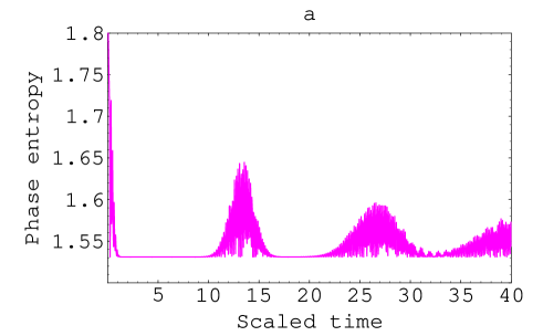
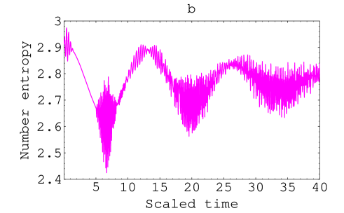
Figure 7: The phase entropy $R_{\psi}$ (a) and the number entropy $R_{N}$ (b) as functions of the scaled time $\lambda_{1}t$ with an initial coherent state of the radiation field with $\bar{n}=20$ based on the exact numerical results due to equation (23). We consider the same parameters as in figure 1.

In figure 7, we plot the number entropy $R_{N}$ and the phase entropy $R_{\psi}$ as functions of the scaled time $\lambda_{1}t$. The initial state of the field is considered as a coherent state. We specifically present the results for the same values of figure 5. It should be noted that at a special choice of the mean-photon number parameter, the situation becomes interesting, where the Rabi frequency has a minimum value at $\bar{n}$. In this case we find that the general behavior of the entropies $R_{N}$ and $R_{\psi}$ and with an initially coherent field exhibit irregular structures instead of the regular structure resembling those manifested by the number or vacuum states cases.

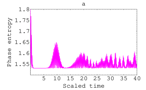
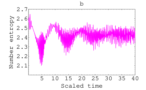
Figure 8: The phase entropy $R_{\psi}$ (a) and the number entropy $R_{N}$ (b) as functions of the scaled time $\lambda_{1}t$ where, $\bar{n}=10$ and the same parameters as in figure 1.

Here it is interesting to note that the periodic oscillations are observed for a short period of the interaction time only. When we consider smaller mean-photon number, the regularity behavior of the oscillations in the entropies $R_{N}$ and $R_{\psi}$ are still obvious (see figure 8) where we have considered the initial mean photon number $\overline{n}=10$. However, the number of oscillations is increased. Also it is interesting to point out that at the revival time optimal phase entropy is attained in all the cases which means that the atom has achieved an almost pure state, this has been observed all through our figures. The number and phase entropic uncertainties for a weak coherent state follow those of underlying states superposition.

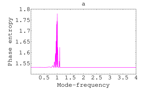
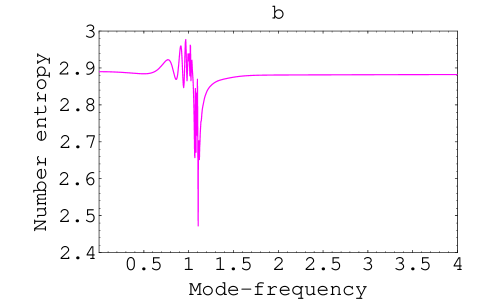
Figure 9: The phase entropy $R_{\psi}$ (a) and the number entropy $R_{N}$ (b) as functions of the mode-frequency $\omega/\omega_{T}$, where, $\bar{n}=20,\lambda_{1}t=\pi/2$.

In figure 9 we plot the entropies $R_{N}$ and $R_{\psi}$ against the mode-frequency $\omega$ in units of $\omega_{T}$ for different values of the scaled time. Now, where the atom-field coupling is proportional to $\lambda_{ij}$ this explains the origin of the second peak in this figure. It is interesting to note the dependence of these entropies on the mode-frequency, with different values of the scaled time. We wonder, as a possible generalization of this concept, whether there exist another family of similar oscillations if we consider two-qubit system. In such a case, the properties of these systems would probably be of interest, in order to bring further insight and knowledge about entanglement and quantum logic gates for multi-partite systems. As the scaled time increased, a characteristic feature of the entropies $R_{N}$ and $R_{\psi}$ is quit interesting, where more oscillations exist, also, only around the resistable region for the number entropy but less number of oscillations exist for the phase entropy (see figure 10).

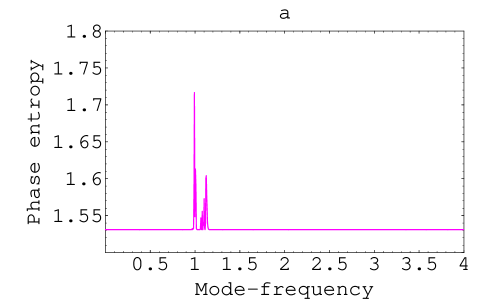
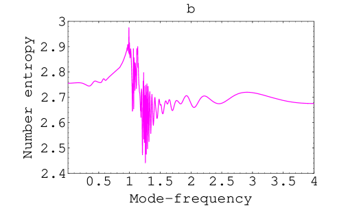
Figure 10: The phase entropy $R_{\psi}$ (a) and the number entropy $R_{N}$ (b) as functions of the mode-frequency $\omega/\omega_{T}$, where, $\bar{n}=20,\lambda_{1}t=3\pi/2$.

Far from the resistable region the entropies behavior observed here does not depend on the mode frequency and the intensity of the initial field mode.

Given a $3D$ photonic crystal with a complete gap, one has the possibility of introducing a defect in the structure which will create a localized state in the gap. If this is a point-like defect then the photon mode will be completely localized about a point. In figure 10, we show the zero point associated with the defect created by removing a small amount of dielectric from one of the vertical dielectric columns of the crystal structure. The resulting defect mode has a state near mid gap. One feature that should be highlighted in this context is the appearance of a frequency gap between the pair of interface dispersion. This gap is present only when the two photonic crystal regions are different, and disappears when they are identical.

5 Experimental prospects

The perfect semiconductor crystal is quite elegant and beautiful, but it becomes ever more useful when it is doped. Likewise, the perfect photonic crystal can become of even greater value when a defect is introduced [32]. The point to make about photonic crystals is that they are very empty structures, consisting of about 78 empty space. But in a sense they are much emptier than that. They are emptier and quieter than even the vacuum, since they contain not even zero-point fluctuations within the forbidden frequency band. Our model system consist of a three-level atom located inside a photonic band gap material. There are several ways of placing such an atom inside a photonic crystal. From a material standpoint, it is possible to dope an existing photonic band gap material using ion beam implantation methods. For instance, it has recently been shown that $Er^{3+}$ ions implanted into bulk silicon exhibit sharp free-atom-like spectra [32, 33]. Intense temperature-dependent photoluminescent (PL) at $1.54{\ \mu}m$ is observed in the system at low temperatures (when the host material is crystalline, Er-related PL is quenched at temperatures above $80K$ so that it cannot be detected at room temperatures). This wavelength is particularly significant because it corresponds to the minimum absorption of silica fibre-based optical communication system. Because the PL at $1.54\mu m$ is due to the spin-orbit split ${}^{4}I_{13/2}\rightarrow^{4}I_{15/2}$ of $4f$ electrons in the $Er^{3+}$ ions which are shielded by outer $5s^{2}5p^{6}$ shells, the influence of the host lattice on the luminescence wavelength is weak. (The key to the success of erbium is that the upper level of the amplifying transition ${}^{4}I_{13/2}$ is separated by a large energy gap from the next-lowest level ${}^{4}I_{15/2}$ so that its lifetime is very long and mostly radiative. In spite of the screening of the atomic transition by the outer shells, it is likely that thermal phonons in the silicon host would cause significant dephasing of the quantum degrees of freedom within the erbium 4f shell. Consequently, such a system must be cooled to liquid helium temperatures. Such experiments appear to be nearly within the reach of current technology. Although it has not yet been demonstrated, the system consisting of a multi-level system coupled to a multi-mode appears to be another potential candidate for achieving new features. Such systems are potentially interesting for their ability to process information in a novel way and might find application in models of quantum logic gates. Therefore, atoms or trapped ions + cavities in a presence of photonic band gap represent, in our opinion, a very promising system for quantum information processing.

6 Conclusion

In this communication the quantum electrodynamic properties of a three-level atom embedded in a photonic band gap material were investigated. We have focused on the application of the effective-medium theory to the present problem in a nanoscale dielectric cavity QED situation. The effective-medium approach can in fact be applied to situations in which all three regions of the structure possess frequency-dependent dielectric functions. Specifically, the combined effects of coherent control by an external driving field and photon localization facilitated by a photonic band gap on entanglement from a three-level atom embedded in a photonic band gap material were examined. Exact solutions of the wave function in the Schrödinger picture have been obtained within rotating wave approximation. In particular, we have chosen to focus on three-level system coupled to a single mode. Observation of the three-level system may offer some insight into the quantum nature of the resonator, just as atoms provide a sensitive probe for the nonclassical nature of electromagnetic fields. The observation of revivals, which are a strictly nonclassical phenomenon, would give evidence for the quantum nature of the quantum system.

The results point to a number of interesting features, which arise from the variation of the adjustable parameters of the system, namely, the mode-frequency, dipole vector orientation, dipole position within the slab, the slab width, and the photonic crystal parameters: layer widths and dielectric functions. Our investigations for the entanglement, collapse-revival phenomena, and phase and number entropic uncertainty relations in the presence of the photonic band gap as compared with the usual three-level model are summarized as follows:-

i) The concurrence behavior is reflect the pattern of collapse and revival which is qualitatively similar to that of the usual three-level model but with reduced amplitude. In case of a smaller mean photon number and for initially excited atom the usual pattern in the three-level model of collapse and revival changes to rapid fluctuations of interference patterns for all time considered. In this way, our concurrence function contains all the information necessary to identify the entanglement of a given state. Nevertheless, it depends on the particular choice of the mode-frequency.

ii) The phase entropy can be used to measure entanglement of the system presented here with explicitly atom-field coupling in the presence of photonic band gap. We would like to point out that the phase Shannon entropic considered for the presented model has not been treated in this manner before.

iii) The photonic band gap introduces sudden changes in the concurrence and phase entropy due to the variation of these quantities with mode frequency. This feature attributed to the fact that in the photonic band gap region electromagnetic modes are not allowed to propagate into the dielectric slab and hence no interaction can take place in this region. Theory predicts analytically this behavior for a GaAs system at $\omega=\eta\omega_{T}$.

Finally, we emphasize the fact that without any conditions it was possible to obtain exact analytic solution which reproduce the most important features of the three-level atom interacting with a cavity one- or two-mode in the presence of photonic band gap. A similar set of equations have been derived in [28] for a three-level system using some approximations, based on the Riccati nonlinear differential equation. In contrast, the method used here gives exact analytic solutions without any conditions.

Acknowledgment

I acknowledge the hospitality and financial support from the Center for Computational and Theoretical Sciences, Kulliyyah of Science, IIUM, Malaysia where the final version of the paper was prepared. Also, helpful discussions with Prof. A.-S. F. Obada and Prof. M. R. B. Wahiddin are gratefully acknowledged.

References

- [1] R.-K. Lee, Y. Lai: J. Opt. B: Quantum Semiclass. Opt. 6, S715 (2004); Jan Perina Jr., C. Sibilia, D. Tricca, M. Bertolotti: Phys. Rev. A 70, 043816 (2004)
- [2] S. Yamada, Y. Watanabe, Y. Katayama, J. B. Cole: J. Appl. Phys. 93, 1859 (2003); 5. S. Yamada, Y. Watanabe, Y. Katayama, X. Y. Yan, J. B. Cole: J. Appl. Phys. 92, 1181 (2002).
- [3] A. Kamli, M. Babiker: Phys. Rev A 62, 043804 (2000).
- [4] J. D. Joannoupoulos, R. B. Meade, J. N. Winn: Photonic Crystals: Molding the Flow of Light (Princeton University Press, Princeton N.J., 1995); S. John: Phys. Rev. Lett. 58 2486 (1987); E. Yablonovitch: Phys. Rev. Lett. 58, 2059 (1987).
- [5] S. John, J. Wang: Phys. Rev. Lett. 64, 2418 (1990).
- [6] S. John, T. Quang: Phys. Rev. A 50, 1764 (1994).
- [7] S.-Y. Zhu, H. Chen, H. Huang: Phys. Rev. Lett. 79, 205 (1997).
- [8] E. Paspalakis, P.L. Knight: Phys. Rev. Lett. 81, 293 (1998)
- [9] E. Paspalakis, N. J. Kylstra, P. L. Knight: Phys. Rev. A 60, R33 (1999).
- [10] M. Florescu, S. John: Phys. Rev. A 64, 033801 (2001).
- [11] G. Vidal, J. I. Latorre, E. Rico, A. Kitaev: Phys. Rev. Lett. 90, 227902 (2003); T. J. Osborne, M. A. Nielsen: Phys. Rev. A 66, 032110 (2002); A. Osterloh, L. Amico, G. Falci, R. Fazio: Nature 416, 608 (2002); I. Bose, E. Chattopadhyay: Phys. Rev. A 66, 062320 (2002).
- [12] V. Buzek, G. Drobny, M. S. Kim, G. Adam, P. L. Knight: Phys. Rev. A 56, 2352 (1997); X. Luo, X. Zhu, Y. Wu, M. Feng, K. Gao, Phys. Lett. A 237, 354 (1998); A. S. Parkins, H. J. Kimble: J.Opt. B: Quantum Semiclass. Opt. 1 , 496 (1999); A. S. Parkins, E. Larsabal: Phys. Rev. A 63, 012304 (2000).
- [13] A. C. Doherty, P. A. Parrilo, F. M. Spedalieri: Phys. Rev. Lett. 88, 187904 (2002); O. Rudolph, quant-ph/0202121; M. Horodecki, P. Horodecki, Horodecki: quant-ph/0206008; for a review see D. Bru ß et. al.: J. Mod. Opt. 49, 1399 (2002).
- [14] A. Peres: Found. Phys. 29, 589 (1999).
- [15] M. Horodecki, P. Horodecki, R. Horodecki: Phys. Lett. A 223, 1 (1996); B.M. Terhal: ibid. 271, 319 (2000); M. Lewenstein et al.: Phys. Rev. A 62, 052310 (2000).
- [16] W. K. Wootters: Phys. Rev. Lett. 80, 2245 (1998); F. Verstraete, K. Audenaert, J.Dehaene, B. De Moor: J. Phys. A: Math. Gen. 34, 10327 (2001); S. Hill, W. Wootters: Phys. Rev. Lett. 80 , 2245 (1998); Opt. Comm.152, 119 (1998); J. Math. Phys. 39 , 4604 (1998).
- [17] I. Bialynicki-Birula, J. Mycielski: Commun. Math. Phys. 44, 129 (1975); D. L. Deutsch, Phys. Rev. Lett. 50, 631 (1983); H. Maassen, J. B. M. Uffink: Phys. Rev. Lett. 60, 1103 (1988).
- [18] J. M. Bendickson, J. P. Dowling: Phys. Rev. E 53, 4107 (1996).
- [19] C. M. Cornelius, J. P. Dowling: Phys. Rev. A 59, 4736 (1999); A. J. Stimpson, J. P. Dowling, Thermal emissivity of 3d photonic band-gap structures, presented at the Optical Society of American Annual Meeting, Long Beach, CA (2001).
- [20] S.-Y. Lin, J. G. Fleming, E. Chow, J. Bur: Phys. Rev. B 62, R2243 (2000).
- [21] S. John, N. Akozbek: Phys. Rev. Lett. 71, 1168 (1993); Phys. Rev. E 57, 2287 (1998).
- [22] A.A. Sukhorukov, Yu.S. Kivshar, O. Bang: Phys. Rev. E 60, R41 (1999).
- [23] A. R. McGurn: Phys. Lett. A 251, 322 (1999); Phys. Lett. A 260, 314 (1999).
- [24] M. Cottam, D. R. Tilley, Introduction to Surface and Superlattice Excitations (Cambridge University Press, Cambridge, England, 1989); V. M. Agranovich, D. L. Mills, Surface Polaritons (North-Holland, Amsterdam, 1982).
- [25] J. A. Kong: Theory of Electromagnetic Waves (Wiley, New York, 1975).
- [26] F. Zolla, D. Felbacq, B. Guizal: Opt. Commum. 148, 6 (1998)
- [27] A. M. Abdel-Hafez, A.-S. F. Obada, M. M. A. Ahmed: Physica A, 144, 530 (1987); A. M. Abdel-Hafez, A. M. M. Abu-Sitta, A.-S. F. Obada: Physica A, 156, 689 (1989); J. H. McGuire, K. K. Shakov, K. Y. Rakhimov: J. Phys. B 36, 3145 (2003)
- [28] S. Bougouffa, A. Kamli: J. Opt. B: Quantum Semiclass. Opt. 6, S60 (2004).
- [29] C. H. Bennett, D. P. DiVincenzo, J. A. Smolin, W.K. Wootters: Phys. Rev. A 54, 3824 (1996); C. H. Bennett, S. J. Wiesner: Phys. Rev. Lett. 69, 2881 (1992); C. H. Bennett, G. Brassard, C. Crepeau, Rjozsa, A. Peres, W. K. Wootters: Phys. Rev. Lett. 70, 1895 (1993).
- [30] P. Rungta, V. Buzek, C. M. Caves, M. Hillery, G. J. Milburn: Phys. Rev. A 64, 042315 (2001); A. Lozinski, A. Buchleitner, K. Zyczkowski, T. Wellens: Europhys. Lett. 62, 168 (2003).
- [31] A.-S. F. Obada, A. M. Abdel-hafez, M. Abdel-Aty: Eur. Phys. J. D 3, 289 (1998); D. T. Pegg, S. M. Barnett: Phys. Rev. A 39, 1065 (1989).
- [32] E Yablonovitch: J. Phys.: Condens. Matter 5, 2443 (1993); M. Woldeyohannes, S. John: J. Opt. B: Quantum Semiclass. Opt. 5, R43 (2003); C. M. Bowden, J. P. Dowling, H. O. Everitt: J. Opt. Soc. Am. B 10, 280 (1993); G. Kurizki, J. W. Haus: Special issue on photonic band structures, J. Mod. Opt. 41, 171 (1994).
- [33] S. Lanzerstorfer, L. Palmetshofer, W. Jantsch, J. Stimmer: Appl. Phys. Lett. 72, 809 (1998); X. Zhao, S. Komuro, H. Isshiki, Y. Aoyagi, T. Sugano: Appl. Phys. Lett. 74 120 (1999).