State space structure and entanglement of rotationally invariant spin systems

Abstract

We investigate the structure of $\mathrm{SO(3)}$-invariant quantum systems which are composed of two particles with spins $j_{1}$ and $j_{2}$. The states of the composite spin system are represented by means of two complete sets of rotationally invariant operators, namely by the projections $P_{J}$ onto the eigenspaces of the total angular momentum $J$, and by certain invariant operators $Q_{K}$ which are built out of spherical tensor operators of rank $K$. It is shown that these representations are connected by an orthogonal matrix whose elements are expressible in terms of Wigner’s $6$-$j$ symbols. The operation of the partial time reversal of the combined spin system is demonstrated to be diagonal in the $Q_{K}$-representation. These results are employed to obtain a complete characterization of spin systems with $j_{1}=1$ and arbitrary $j_{2}\geq 1$. We prove that the Peres-Horodecki criterion of positive partial transposition (PPT) is necessary and sufficient for separability if $j_{2}$ is an integer, while for half-integer spins $j_{2}$ there always exist entangled PPT states (bound entanglement). We construct an optimal entanglement witness for the case of half-integer spins and design a protocol for the detection of entangled PPT states through measurements of the total angular momentum.

I Introduction

Entanglement is a basic feature of composite quantum systems connected to the tensor product structure of the underlying Hilbert space of states. A mixed state of a bipartite quantum system described by some density matrix $\rho$ is said to be entangled or inseparable if $\rho$ cannot be written as a convex linear combination of product states. Otherwise it is called classically correlated or separable WERNER . The properties of entangled states are responsible for many of the fascinating and curious aspects of the quantum world and lie at the core of many proposed applications in quantum information processing ECKERT ; ALBER ; NIELSEN .

The general characterization and quantification of entanglement in mixed quantum states is a highly non-trivial problem. It is even very difficult in general to formulate simple operational criteria which allow a unique identification of all separable states of a given composite system. There do exist, however, many necessary separability criteria PERES ; HORODECKI96a ; HORODECKI99 ; CERF ; KEMPE ; RUDOLPH03 ; CHEN ; TERHAL ; LEWENSTEIN00 . A simple and, in fact, very strong criterion is the Peres-Horodecki criterion PERES ; HORODECKI96a which states that a necessary condition for a given density matrix $\rho$ to be separable is that it has a positive partial transposition (PPT states). It is known that this criterion is necessary and sufficient for certain low-dimensional systems, while it is only necessary in higher dimensions HORODECKI96a .

The analysis of the entanglement structure is greatly facilitated through the introduction of symmetries, i. e., if one restricts to those states of the composite system which are invariant under certain groups of symmetry transformations. Important examples in this context are the manifolds of the Werner states WERNER , of the isotropic states RAINS ; HORODECKI99 and of the orthogonal states VOLLBRECHT . Here, we investigate entanglement under the symmetry group $\mathrm{SO(3)}$ of proper three-dimensional rotations of the coordinate axes. More precisely, we consider the problem of mixed state entanglement of systems which are composed of two particles with spins $j_{1}$ and $j_{2}$, and which are invariant under product representations of the group $\mathrm{SO(3)}$ or, equivalently, of the covering group $\mathrm{SU(2)}$. A basic tool of our analysis is the work of Vollbrecht and Werner VOLLBRECHT which provides a general scheme for the treatment of entanglement under given symmetry groups.

Mixed $\mathrm{SO(3)}$-invariant states of composite systems arise, for example, from the interaction of open systems TheWork with isotropic environments GORINI . Their analysis is of great importance and leads to many applications. As examples we mention investigations on the connection between quantum phase transitions and the behaviour of entanglement measures (see, e. g., OSTERLOH ; OSBORNE ), the analysis of entanglement of $\mathrm{SU(2)}$-invariant multiphoton states generated by parametric down-conversion DURKIN , and studies of the entanglement of formation CAVES . The technique of this paper could also be relevant for the characterization of quantum correlations in Fermionic or Bosonic systems developed recently SCHLIEMANN01 ; BRUSS .

The Hilbert space of a system which is composed of two particles with spins $j_{1}$ and $j_{2}$ is given by the tensor product ${\mathbb{C}}^{N_{1}}\otimes{\mathbb{C}}^{N_{2}}$, where $N_{1}=2j_{1}+1$ and $N_{2}=2j_{2}+1$ are the dimensions of the local spin spaces. We call such a system an $N_{1}\otimes N_{2}$ system. Throughout the paper we will assume that $j_{1}\leq j_{2}$, i. e., $N_{1}\leq N_{2}$.

According to the Peres-Horodecki criterion PERES ; HORODECKI96a the cases of $2\otimes 2$ and $2\otimes 3$ systems are trivial: It is known that in these cases the PPT criterion is necessary and sufficient for all states, i. e., even for states which are not invariant under rotations. Schliemann SCHLIEMANN1 has shown recently that the PPT criterion is also necessary and sufficient for $\mathrm{SO(3)}$-invariant $2\otimes N_{2}$ systems with arbitrary $N_{2}$. The case of $3\otimes 3$ systems has been treated by Vollbrecht and Werner VOLLBRECHT , who proved that the PPT criterion is again necessary and sufficient for separability. For $4\otimes 4$ systems a qualitatively new situation arises: It has been demonstrated in NtensorN that the PPT criterion is not sufficient and that the entangled PPT states form a three-dimensional manifold which is isomorphic to a prism. In the present work we investigate the important special case of $3\otimes N_{2}$ systems with arbitrary $N_{2}$.

The method developed in NtensorN enables the treatment of the case of equal spins $j_{1}=j_{2}$. In this paper we extend this method to arbitrary spins $j_{1}$ and $j_{2}$. For the analysis of entanglement under $\mathrm{SO(3)}$-symmetry it is advantageous to replace the transposition used in the PPT criterion by another unitarily equivalent operation, namely by the antiunitary transformation of the time reversal. The reason for this fact is that the operation of the time reversal of states commutes with the representations of the rotation group.

There are two natural representations of rotationally invariant states. The first one uses the fact that any invariant state can be written as a unique convex linear combination of the projections $P_{J}$ onto the eigenspaces of the total angular momentum $J$ of the composite spin system. The advantage of this representation is that it leads to very simple conditions expressing the positivity and the normalization of physical states. However, the set of the PPT states is most easily determined in another representation which employs the irreducible spherical tensor operators of spin-$j$ particles. We will construct a complete system of invariant operators $Q_{K}$ which are built out of the spherical tensors of rank $K$. Any invariant state of the composite spin system can then be written as a unique linear combination of the $Q_{K}$. The introduction of the invariant operators $Q_{K}$ generalizes the ideas of Schliemann SCHLIEMANN1 ; SCHLIEMANN2 , who has developed a representation of $\mathrm{SU(2)}$-invariant states by means of spin-spin correlators and has formulated various separability conditions and sum rules in terms of these correlators.

The paper is organized as follows. The representations of $\mathrm{SO(3)}$-invariant states in terms of the invariant operators $P_{J}$ and $Q_{K}$ are constructed in Sec. II. We also derive in this section the linear transformation which connects these representations and show that it is given by an orthogonal matrix whose elements are determined by Wigner’s $6$-$j$ symbols. The behaviour of states under partial time reversal and the construction of the set of the invariant separable states are discussed in Sec. III.

The general theory is then applied in Sec. IV to the case of $3\otimes N_{2}$ systems with arbitrary $N_{2}$. We prove that the PPT criterion represents a necessary and sufficient separability condition for $3\otimes N_{2}$ systems if and only if $N_{2}$ is odd. Thus, for integer spins $j_{2}$ all PPT states are separable, while for half-integer spins $j_{2}$ there always exist entangled PPT states. This fact has already been conjectured by Hendriks HENDRIKS on the basis of a detailed numerical investigation. We also show that for half-integer $j_{2}$ the boundary of the separability region is curved. Finally, Sec. V contains a discussion of the results and some conclusions. In particular, we construct an optimal entanglement witness for the case of half-integer spins and exploit this witness to design a protocol which allows the detection of entangled PPT states through measurements of the total angular momentum.

II Representations of $\mathrm{SO(3)}$-invariant states

We consider two particles with spins $j_{1}$ and $j_{2}$ and corresponding angular momentum operators $\hat{\bm{j}}^{(1)}$ and $\hat{\bm{j}}^{(2)}$. The Hilbert space ${\mathbb{C}}^{N_{1}}$ of the first particle is spanned by the common eigenstates $|j_{1},m_{1}\rangle$ of the square of $\hat{\bm{j}}^{(1)}$ and of $\hat{\bm{j}}^{(1)}_{z}$, where $N_{1}\equiv 2j_{1}+1$ and $m_{1}=-j_{1},\ldots,+j_{1}$. Correspondingly, the Hilbert space ${\mathbb{C}}^{N_{2}}$ of the second particle is spanned by the eigenstates $|j_{2},m_{2}\rangle$, where $N_{2}\equiv 2j_{2}+1$ and $m_{2}=-j_{2},\ldots,+j_{2}$.

The Hilbert space of the total system composed of both particles is given by the tensor product ${\mathbb{C}}^{N_{1}}\otimes{\mathbb{C}}^{N_{2}}$. The angular momentum operator of the composite system is defined by:

$$\hat{\bm{J}}=\hat{\bm{j}}^{(1)}\otimes I+I\otimes\hat{\bm{j}}^{(2)},$$ (1)

where $I$ denotes the unit matrix. A state of the composite system is described by a density matrix on the product space, i. e., by a positive operator $\rho$ on ${\mathbb{C}}^{N_{1}}\otimes{\mathbb{C}}^{N_{2}}$ with unit trace: $\rho\geq 0$, ${\mathrm{tr}}\rho=1$.

The irreducible unitary representation of the group $\mathrm{SO(3)}$ of proper rotations $R$ on the state space of a particle with spin $j$ will be denoted by $D^{(j)}(R)$. The transformation of the states of the composite spin system is then given by the product representation $D^{(j_{1})}(R)\otimes D^{(j_{2})}(R)$. A state $\rho$ of the combined system is said to be rotationally invariant or $\mathrm{SO(3)}$-invariant if the relation

$$\left[D^{(j_{1})}(R)\otimes D^{(j_{2})}(R)\right]\rho\left[D^{(j_{1})}(R)\otimes D^{(j_{2})}(R)\right]^{\dagger}=\rho$$

holds true for all proper rotations $R\in SO(3)$.

We shall use two different representations of rotationally invariant states. The first one employs the projection operators

$$P_{J}=\sum_{M=-J}^{+J}|JM\rangle\langle JM|,$$ (2)

where $|JM\rangle$ denotes the common eigenstate of the square of the total angular momentum $\hat{\bm{J}}$ and of its $z$-component $\hat{J}_{z}$, i. e., we have $\hat{\bm{J}}^{2}|JM\rangle=J(J+1)|JM\rangle$ and $\hat{J}_{z}|JM\rangle=M|JM\rangle$. The operator $P_{J}$ projects onto the manifold which is spanned by the eigenstates belonging to a fixed value $J$ of the total angular momentum. According to the triangular inequality $J$ takes on $N_{1}$ different values which may be integer or half-integer valued:

$$J=j_{2}-j_{1},j_{2}-j_{1}+1,\ldots,j_{2}+j_{1}.$$ (3)

It follows from Schur’s lemma that any invariant state $\rho$ can be written as a linear combination of the $P_{J}$:

$$\rho=\frac{1}{\sqrt{N_{1}N_{2}}}\sum_{J}\frac{\alpha_{J}}{\sqrt{2J+1}}P_{J}.$$ (4)

Here, the $\alpha_{J}$ are real parameters and we have introduced convenient normalization factors of $\sqrt{N_{1}N_{2}}$ and $\sqrt{2J+1}$. In order for Eq. (4) to represent a true density matrix the $\alpha_{J}$ must of course be positive and normalized appropriately:

$$\alpha_{J} \geq 0,$$ (5)

$${\mathrm{tr}}\rho = \sum_{J}\sqrt{\frac{2J+1}{N_{1}N_{2}}}\alpha_{J}=1.$$ (6)

Any invariant state $\rho$ is thus uniquely characterized by a real vector $\bm{\alpha}$ in an $N_{1}$-dimensional parameter space ${\mathbb{R}}^{N_{1}}$ which will be referred to as $\alpha$-space. The conditions of the positivity and of the normalization of $\rho$ are expressed by the relations (5) and (6). We denote the set of all vectors $\bm{\alpha}$ whose components $\alpha_{J}$ satisfy these relations by $S^{\alpha}$. Being isomorphic to the set of invariant states, $S^{\alpha}$ is of course a convex set. We infer from Eqs. (5) and (6) that $S^{\alpha}$ represents an $(N_{1}-1)$-dimensional simplex.

A useful alternative representation of the invariant states is obtained by use of a complete system of irreducible spherical tensor operators (see, e. g. EDMONDS ; SCHWINGER ). The tensor operators which act on the state space of the particle with spin $j_{i}$ are written as $T^{(i)}_{K_{i}q_{i}}$, where $i=1,2$. The index $K_{i}=0,1,\ldots,2j_{i}$ denotes the rank of the tensor operator. For a given rank $K_{i}$ the index $q_{i}$ takes on the values $q_{i}=-K_{i},-K_{i}+1,\ldots,+K_{i}$. We thus have $(2K_{i}+1)$ tensor operators $T^{(i)}_{K_{i}q_{i}}$ of rank $K_{i}$ which transform under rotations according to an irreducible representation of the rotation group. The explicit definitions of the tensors and a brief summary of their properties are given in Appendix A.

Using the tensor operators one defines Hermitian operators $Q_{K}$ acting on the state space of the composite spin system:

$$Q_{K}=\sum_{q=-K}^{+K}T^{(1)}_{Kq}\otimes T^{(2)\dagger}_{Kq},$$ (7)

where the index $K$ takes on $N_{1}$ different integer values:

$$K=0,1,\ldots,2j_{1}.$$ (8)

It follows from the transformation properties of the tensor operators that all $Q_{K}$ are invariant under rotations. For instance, the operator $Q_{0}$ is proportional to the identity, $Q_{0}=\frac{1}{\sqrt{N_{1}N_{2}}}I\otimes I$, while $Q_{1}$ is proportional to the invariant scalar product $\hat{\bm{j}}^{(1)}\cdot\hat{\bm{j}}^{(2)}$ of the spin vectors.

The $Q_{K}$ defined by Eq. (7) form a complete system of operators. This means that any rotationally invariant Hermitian operator can be represented as a unique linear combination of the $Q_{K}$ in a way analogous to Eq. (4):

$$\rho=\frac{1}{\sqrt{N_{1}N_{2}}}\sum_{K}\frac{\beta_{K}}{\sqrt{2K+1}}Q_{K}.$$ (9)

Here, we have again introduced appropriate normalization factors and real parameters $\beta_{K}$ which form a vector $\bm{\beta}$ in an $N_{1}$-dimensional parameter space ${\mathbb{R}}^{N_{1}}$ referred to as $\beta$-space. The operators $Q_{K}$ satisfy ${\mathrm{tr}}\{Q_{K}Q_{K^{\prime}}\}=(2K+1)\delta_{KK^{\prime}}$. This fact follows directly from the orthogonality relation (76) for the spherical tensors. The $Q_{K}$ for $K\neq 0$ are therefore traceless which leads to the normalization condition

$${\mathrm{tr}}\rho=\beta_{0}=1.$$ (10)

The sets $\{P_{J}\}$ and $\{Q_{K}\}$ represent complete systems of invariant operators. The corresponding parameter vectors $\bm{\alpha}$ and $\bm{\beta}$ must therefore be related by a linear transformation ${\mathbb{R}}^{N_{1}}\mapsto{\mathbb{R}}^{N_{1}}$. We write

$${\bm{\beta}}=L{\bm{\alpha}},$$ (11)

where $L$ is an $(N_{1}\times N_{1})$ matrix. To find the elements of this matrix we use Eqs. (4) and (9) to get

$$\sum_{J}\frac{\alpha_{J}}{\sqrt{2J+1}}P_{J}=\sum_{K}\frac{\beta_{K}}{\sqrt{2K+1}}Q_{K}.$$ (12)

Multiplying this equation by $Q_{K^{\prime}}$ and taking the trace we find that the elements of $L$ are given by

$$L_{KJ}=[(2K+1)(2J+1)]^{-1/2}{\mathrm{tr}}\{Q_{K}P_{J}\}.$$ (13)

This can be expressed as

$$L_{KJ}=\sqrt{(2K+1)(2J+1)}(-1)^{j_{1}+j_{2}+J}\left\{\begin{array}[]{ccc}j_{1}&j_{2}&J\\ j_{2}&j_{1}&K\end{array}\right\}.$$ (14)

The curly brackets denote a $6$-$j$ symbol introduced by Wigner WIGNER into the quantum theory of angular momentum. A proof of the relation (14) is given in Appendix B. The $6$-$j$ symbols are scalar quantities which are defined through invariant sums over products of Clebsch-Gordan coefficients. They describe the transformation between different coupling schemes for the addition of three angular momenta EDMONDS . Their properties have been studied in great detail and many closed formulae, recursion relations and sum rules are known. In particular, it follows from the sum rules that $L$ represents an orthogonal $(N_{1}\times N_{1})$ matrix.

The above results lead to the conclusion that the set of $\mathrm{SO(3)}$-invariant states is represented in $\beta$-space by the set

$$S^{\beta}=LS^{\alpha}.$$ (15)

The set $S^{\beta}$ is again an $(N_{1}-1)$-dimensional simplex which may be constructed by determining the images of the extreme points of $S^{\alpha}$ under the orthogonal transformation $L$.

The introduction of two parameter spaces is motivated by the following observations. On the one hand, the set of states is most easily constructed as a subset in $\alpha$-space. This is due to the fact that the representation of Eq. (4) corresponds to the spectral decomposition of $\rho$ and, therefore, the requirement of the positivity of $\rho$ immediately leads to the simple condition (5). On the other hand, the representation (9) of states in $\beta$-space is much more suitable for the construction of the set of separable states, which is due to the fact that the operation of the partial time reversal is diagonal in the $Q_{K}$-representation.

III Invariant separable states

A state $\rho$ of the composite spin system is said to be separable if it is possible to write this state as a convex linear combination of product states:

$$\rho=\sum_{i}\lambda_{i}\rho_{i}^{(1)}\otimes\rho_{i}^{(2)},\qquad\lambda_{i}\geq 0,\qquad\sum_{i}\lambda_{i}=1,$$ (16)

where the $\rho_{i}^{(1)}$ and $\rho_{i}^{(2)}$ are normalized states of the first and of the second spin, respectively WERNER . It is clear that the set in $\beta$-space which represents the invariant and separable states is a convex subset of $S^{\beta}$. This subset will be denoted by $S^{\beta}_{\mathrm{sep}}$.

Following the work of Vollbrecht and Werner VOLLBRECHT we define a projection super-operator ($\mathrm{SO(3)}$ twirling) by means of

$$\Pi\rho=\int dR\;U(R)\rho U(R)^{\dagger},$$ (17)

where $U(R)\equiv D^{(j_{1})}(R)\otimes D^{(j_{2})}(R)$ and the integration is extended over all group elements $R\in SO(3)$. The twirl operation maps any state $\rho$ of the composite spin system to an $\mathrm{SO(3)}$-invariant state $\Pi\rho$. Moreover, if $\rho$ is separable then also $\Pi\rho$ is separable. In terms of the invariant operators $P_{J}$ or $Q_{K}$ the action of the twirl operation may be expressed by

$$\Pi\rho=\sum_{J}\frac{{\mathrm{tr}}\{P_{J}\rho\}}{2J+1}P_{J}=\sum_{K}\frac{{\mathrm{tr}}\{Q_{K}\rho\}}{2K+1}Q_{K}.$$ (18)

It is known that any invariant separable state is a convex linear combination of $\Pi$-projections of pure product states. Given a pure product state

$$\rho=|\varphi^{(1)}\varphi^{(2)}\rangle\langle\varphi^{(1)}\varphi^{(2)}|,$$ (19)

Eq. (18) shows that the corresponding parameters $\alpha_{J}$ and $\beta_{K}$ of its projection $\Pi\rho$ are given by

$$\alpha_{J} = \sqrt{\frac{N_{1}N_{2}}{2J+1}}\langle\varphi^{(1)}\varphi^{(2)}|P_{J}|\varphi^{(1)}\varphi^{(2)}\rangle,$$ (20)

$$\beta_{K} = \sqrt{\frac{N_{1}N_{2}}{2K+1}}\langle\varphi^{(1)}\varphi^{(2)}|Q_{K}|\varphi^{(1)}\varphi^{(2)}\rangle.$$ (21)

We introduce into Eq. (21) the definition (7) of the $Q_{K}$ and define the functions

$$\tilde{\beta}_{K}[\varphi^{(1)},\varphi^{(2)}]$$

$$=\sqrt{\frac{N_{1}N_{2}}{2K+1}}\sum_{q=-K}^{+K}\langle\varphi^{(1)}|T^{(1)}_{Kq}|\varphi^{(1)}\rangle\langle\varphi^{(2)}|T^{(2)\dagger}_{Kq}|\varphi^{(2)}\rangle.$$

Let us further define $W^{\beta}$ as the range of the parameter vector $\bm{\beta}$ whose components are given by these functions, where $|\varphi^{(1)}\rangle\in{\mathbb{C}}^{N_{1}}$ and $|\varphi^{(2)}\rangle\in{\mathbb{C}}^{N_{2}}$ run independently over all normalized states of the first and of the second spin, respectively:

$$W^{\beta}=\left\{\bm{\beta}\left|\;\beta_{K}=\tilde{\beta}_{K}[\varphi^{(1)},\varphi^{(2)}],\;||\varphi^{(1,2)}||=1\right.\right\}.$$ (23)

The set of separable states is then equal to the convex hull of $W^{\beta}$:

$$S^{\beta}_{\mathrm{sep}}={\mbox{hull}}\left(W^{\beta}\right).$$ (24)

This means that $S^{\beta}_{\mathrm{sep}}$ is equal to the smallest convex set which contains $W^{\beta}$.

Within this formulation the problem of constructing $S^{\beta}_{\mathrm{sep}}$ reduces to the determination of the convex hull of the range of the functions $\tilde{\beta}_{K}$. Even for the present case of a highly symmetric state space this is, in general, an extremely difficult task. A strong necessary condition for separability is the Peres-Horodecki criterion PERES ; HORODECKI96a . According to this criterion a necessary condition for a given state $\rho$ to be separable is that its partial transposition is a positive operator: $T_{2}\rho\equiv(I\otimes T)\rho\geq 0$. Here, $TB=B^{T}$ denotes the transposition of the operator $B$ on ${\mathbb{C}}^{N_{2}}$ which is defined in terms of the basis states of the second spin by means of $\langle j_{2},m_{2}|B^{T}|j_{2},m^{\prime}_{2}\rangle=\langle j_{2},m^{\prime}_{2}|B|j_{2},m_{2}\rangle$. The partial transposition $T_{2}$ is then defined by $T_{2}(A\otimes B)=A\otimes B^{T}$.

The operation of taking the partial transposition destroys the rotational invariance of states, i. e., if $\rho$ is invariant under rotations the partially transposed state $T_{2}\rho$ is generally not $\mathrm{SO(3)}$-invariant. However, there exist another operation which is unitarily equivalent to $T_{2}$ and which does map rotationally invariant operators to rotationally invariant operators. This operation will be denoted by $\vartheta_{2}=I\otimes\vartheta$. It involves the antiunitary time reversal transformation $\vartheta$ of the second spin and will therefore be referred to as partial time reversal.

According to Wigner’s representation theorem WIGNER the action of the time reversal transformation $\vartheta$ on an operator $B$ can be expressed as:

$$\vartheta B=VB^{T}V^{\dagger}=\tau B^{\dagger}\tau^{-1}.$$ (25)

In the first expression $T$ denotes again the transposition and $V$ is a unitary matrix which represents a rotation of the coordinate system about the $y$-axis by the angle $\pi$. In the second expression of Eq. (25) $\tau$ denotes the operator $\tau=V\tau_{0}$ which is composed of the $\pi$-rotation $V$ and of the operator $\tau_{0}$ of the complex conjugation. The operator $\tau$ is antiunitary and satisfies

$$\tau^{2}=(-1)^{2j_{2}}.$$ (26)

$\vartheta$ is a positive but not completely positive map. It is unitarily equivalent to the transposition $T$ and, hence, the Peres-Horodecki criterion can be expressed by

$$\vartheta_{2}\rho\equiv(I\otimes\vartheta)\rho\geq 0.$$ (27)

A great advantage of the representation of states in $\beta$-space is that the operators $Q_{K}$ have a very simple behaviour under the map $\vartheta_{2}$. Namely, as is shown in Appendix A they are eigenoperators of the partial time reversal: $\vartheta_{2}Q_{K}=(-1)^{K}Q_{K}$. In $\beta$-space the map $\vartheta_{2}$ therefore induces a reflection of the coordinate axes corresponding to the odd values of $K$:

$$\vartheta_{2}:\;\beta_{K}\mapsto(-1)^{K}\beta_{K}.$$ (28)

We thus get the image $\vartheta_{2}S^{\beta}$ of $S^{\beta}$ by reversing the signs of the odd coordinates.

We define $S^{\beta}_{\mathrm{ppt}}$ as the set of states which are positive under $\vartheta_{2}$ or, equivalently, under $T_{2}$ (PPT states). This set is equal to the intersection of $S^{\beta}$ with its image $\vartheta_{2}S^{\beta}$. According to the Peres-Horodecki criterion the set of separable states is a subset of the set of PPT states. Hence, we have

$$S^{\beta}_{\mathrm{sep}}\subset S^{\beta}_{\mathrm{ppt}}=S^{\beta}\cap\vartheta_{2}S^{\beta}.$$ (29)

We note three properties which turn out to be useful in the construction of the set of separable states.

(1) The functions defined by Eq. (III) are invariant under simultaneous rotations of the input arguments:

$$\tilde{\beta}_{K}[D^{(j_{1})}(R)\varphi^{(1)},D^{(j_{2})}(R)\varphi^{(2)}]=\tilde{\beta}_{K}[\varphi^{(1)},\varphi^{(2)}].$$ (30)

This property is an immediate consequence of the rotational invariance of the operators $Q_{K}$.

(2) The range $W^{\beta}$ defined in Eq. (23) is obviously invariant under the partial time reversal $\vartheta_{2}$. This means that $\bm{\beta}\in W^{\beta}$ implies $\vartheta_{2}\bm{\beta}\in W^{\beta}$.

(3) There exist two distinguished separable states. These are the state given by the parameter vector $\bm{\alpha}$ with components

$$\alpha_{J}=\sqrt{\frac{N_{1}N_{2}}{2J_{\max}+1}}\delta_{J,J_{\max}},\qquad J_{\max}\equiv j_{1}+j_{2},$$ (31)

and the partially time reversed state given by $\bm{\alpha}^{\prime}=\vartheta_{2}\bm{\alpha}$. To proof this statement we consider a pure product state $\rho$ of the form of Eq. (19) with $|\varphi^{(1)}\rangle=|j_{1},+j_{1}\rangle$ and $|\varphi^{(2)}\rangle=|j_{2},+j_{2}\rangle$. We then have the obvious relation $|J=J_{\max},M=+J_{\max}\rangle=|\varphi^{(1)}\varphi^{(2)}\rangle$ and, hence,

$$\langle\varphi^{(1)}\varphi^{(2)}|P_{J}|\varphi^{(1)}\varphi^{(2)}\rangle=\delta_{J,J_{\max}}.$$ (32)

Equation (20) then immediately leads to Eq. (31). This means that the pure product state $\rho$ is mapped under the twirl operation to the separable state $\Pi\rho=\frac{1}{2J_{\max}+1}P_{J_{\max}}$ corresponding to the maximal value of the total angular momentum $J_{\max}$. It follows from point (2) that also the partially time reversed state is separable.

The point $\bm{\alpha}$ given by Eq. (31) is an extreme point of the simplex $S^{\alpha}$ and its image $\bm{\alpha}^{\prime}$ is an extreme point of $\vartheta_{2}S^{\alpha}$. Thus, $\bm{\alpha}$ and $\bm{\alpha}^{\prime}$ are extreme points of $S^{\alpha}_{\mathrm{ppt}}$. It follows that the corresponding points $\bm{\beta}=L\bm{\alpha}$ and $\bm{\beta}^{\prime}=L\bm{\alpha}^{\prime}$ in $\beta$-space belong to $W^{\beta}$ and represent extreme points of $S^{\beta}_{\mathrm{ppt}}$.

As an illustration of the above analysis consider a $2\otimes N_{2}$ system for which $j_{1}=\frac{1}{2}$ and $j_{2}$ is arbitrary. As has been demonstrated by Schliemann SCHLIEMANN1 the PPT criterion is a necessary and sufficient separability condition in this case. Within the present formulation this statement can be proven as follows. We first note that the index $K$ takes on the two values $K=0,1$ such that $\bm{\beta}$ is a two-dimensional vector. Because of the normalization condition (10) we only need a single parameter $\beta_{1}$ to characterize uniquely an invariant state of a $2\otimes N_{2}$ system. It follows that $S^{\beta}$ can be represented by an interval of the $\beta_{1}$-axis, and $S^{\beta}_{\mathrm{ppt}}$ by a sub-interval of this interval. Since an interval has exactly two extreme points (its endpoints) we conclude with the help of point (3) above that the extreme points of $S^{\beta}_{\mathrm{ppt}}$ belong to $W^{\beta}$. By the relation (24) the sets $S^{\beta}_{\mathrm{ppt}}$ and $S^{\beta}_{\mathrm{sep}}$ therefore coincide. This shows that the PPT criterion is indeed necessary and sufficient for separability.

IV $3\otimes N$ systems

Let us now consider the case $j_{1}=1$ ($N_{1}=3$) and $j_{2}$ arbitrary, i. e. the case of $3\otimes N_{2}$ systems. For convenience we write $N\equiv N_{2}=2j_{2}+1$. Since $J$ takes on the values $J=j_{2}-1$, $j_{2}$ and $j_{2}+1$, $\bm{\alpha}$ is a three-vector

$$\bm{\alpha}=\left(\begin{array}[]{c}\alpha_{j_{2}-1}\\ \alpha_{j_{2}}\\ \alpha_{j_{2}+1}\end{array}\right).$$ (33)

The set $S^{\alpha}$ of invariant states is given by the relations:

$$\alpha_{j_{2}-1},\alpha_{j_{2}},\alpha_{j_{2}+1}\geq 0$$ (34)

and

$$\sqrt{\frac{N-2}{3N}}\alpha_{j_{2}-1}+\sqrt{\frac{1}{3}}\alpha_{j_{2}}+\sqrt{\frac{N+2}{3N}}\alpha_{j_{2}+1}=1.$$ (35)

We observe that $S^{\alpha}$ is a 2-simplex, i. e. a triangle whose vertices are given by the following parameter vectors $\bm{\alpha}$:

$$\left(\begin{array}[]{c}0\\ 0\\ \sqrt{\frac{3N}{N+2}}\end{array}\right),\qquad\left(\begin{array}[]{c}\sqrt{\frac{3N}{N-2}}\\ 0\\ 0\end{array}\right),\qquad\left(\begin{array}[]{c}0\\ \sqrt{3}\\ 0\end{array}\right).$$ (36)

In order to transform to $\beta$-space we first determine the matrix $L$ by means of the formulae (102)-(104):

$$L=$$

$$\left[\begin{array}[]{ccc}\sqrt{\frac{N-2}{3N}}&\sqrt{\frac{1}{3}}&\sqrt{\frac{N+2}{3N}}\\ -\sqrt{\frac{(N-2)(N+1)}{2N(N-1)}}&-\sqrt{\frac{2}{(N-1)(N+1)}}&\sqrt{\frac{(N-1)(N+2)}{2N(N+1)}}\\ \sqrt{\frac{(N+1)(N+2)}{6N(N-1)}}&-\sqrt{\frac{2(N-2)(N+2)}{3(N-1)(N+1)}}&\sqrt{\frac{(N-1)(N-2)}{6N(N+1)}}\end{array}\right].$$

The extreme points of $S^{\beta}$ are found by applying this matrix to the vectors given in Eq. (36). Since $\beta_{0}$ is identically equal to $1$ by the normalization condition (10) we can represent points in $\beta$-space by two coordinates $(\beta_{1},\beta_{2})$. One finds that $S^{\beta}$ is a triangle in the $(\beta_{1},\beta_{2})$-plane with the vertices:

$$A=\left(\sqrt{\frac{3(N-1)}{2(N+1)}},\sqrt{\frac{(N-1)(N-2)}{2(N+1)(N+2)}}\right),$$ (38)

$$B=\left(-\sqrt{\frac{3(N+1)}{2(N-1)}},\sqrt{\frac{(N+1)(N+2)}{2(N-1)(N-2)}}\right),$$ (39)

$$C=\left(-\sqrt{\frac{6}{(N-1)(N+1)}},-\sqrt{\frac{2(N-2)(N+2)}{(N-1)(N+1)}}\right).$$ (40)

Figure 1: State space structure of a system composed of two particles with spins $j_{1}=1$ and $j_{2}=\frac{3}{2}$ ($N=4$). The triangle $ABC$ represents the set $S^{\beta}$ of invariant states, while the triangle $\vartheta_{2}S^{\beta}$ is its image under the partial time reversal. The polygon $AA^{\prime}DE$ represents the set $S^{\beta}_{\mathrm{ppt}}$ of the PPT states.

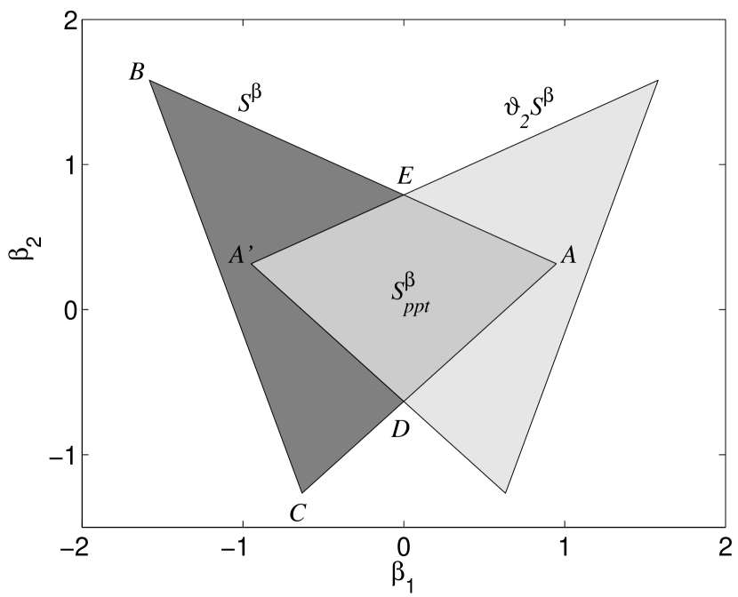
The image $\vartheta_{2}S^{\beta}$ of $S^{\beta}$ under the partial time reversal is obtained by reversing the sign of the coordinate $\beta_{1}$. Consequently, $S^{\beta}_{\mathrm{ppt}}$ is a polygon with the four vertices $A$, $A^{\prime}$, $D$ and $E$, where $A$ is given by Eq. (38) and:

$$A^{\prime} = \left(-\sqrt{\frac{3(N-1)}{2(N+1)}},\sqrt{\frac{(N-1)(N-2)}{2(N+1)(N+2)}}\right),$$ (41)

$$D = \left(0,-\sqrt{\frac{2(N-1)(N-2)}{(N+1)(N+2)}}\right),$$ (42)

$$E = \left(0,\sqrt{\frac{(N+1)(N-1)}{2(N+2)(N-2)}}\right).$$ (43)

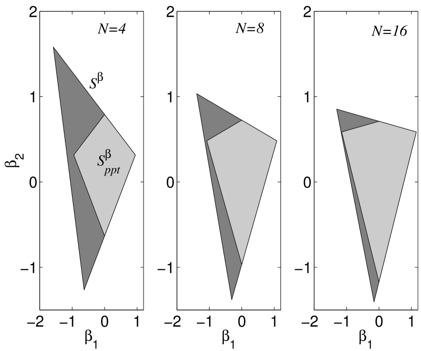
Here, $A^{\prime}=\vartheta_{2}A$ is the image of $A$ under $\vartheta_{2}$, while $D$ and $E$ are the intersections of the lines $AC$ and $AB$ with the $\beta_{2}$-axis, respectively. The case $N=4$ is illustrated in Fig. 1. Similar pictures are obtained for other values of $N$. Examples are shown in Fig. 2. Note that the origin of the $(\beta_{1},\beta_{2})$-plane describes the state $\rho=\frac{1}{3N}I\otimes I$ of maximal entropy.

Figure 2: The sets of the invariant states $S^{\beta}$ and of the invariant PPT states $S^{\beta}_{\mathrm{ppt}}$ for three different values of $N$.

To construct the set $S^{\beta}_{\mathrm{sep}}$ of separable states we have to investigate the functions:

$$\tilde{\beta}_{1}[\varphi^{(1)},\varphi^{(2)}]$$

$$=\sqrt{N}\sum_{q=-1}^{+1}\langle\varphi^{(1)}|T^{(1)}_{1q}|\varphi^{(1)}\rangle\langle\varphi^{(2)}|T^{(2)\dagger}_{1q}|\varphi^{(2)}\rangle$$

and

$$\tilde{\beta}_{2}[\varphi^{(1)},\varphi^{(2)}]$$

$$=\sqrt{\frac{3N}{5}}\sum_{q=-2}^{+2}\langle\varphi^{(1)}|T^{(1)}_{2q}|\varphi^{(1)}\rangle\langle\varphi^{(2)}|T^{(2)\dagger}_{2q}|\varphi^{(2)}\rangle.$$

We distinguish two cases, namely the cases of odd and of even $N$.

Theorem 1

For integer spins $j_{2}=1,2,3,\ldots$ one has $S^{\beta}_{\mathrm{ppt}}=S^{\beta}_{\mathrm{sep}}$. Hence, for all $3\otimes N$ systems with odd $N$ the PPT criterion represents a necessary and sufficient condition for the separability of rotationally invariant states.

To proof this theorem we show that the vertices $A$, $A^{\prime}$, $D$ and $E$ of the polygon $S^{\beta}_{\mathrm{ppt}}$ belong to $W^{\beta}$. The statement $S^{\beta}_{\mathrm{ppt}}=S^{\beta}_{\mathrm{sep}}$ then follows immediately from Eq. (24).

The point $A$ corresponds to the parameter vector $\bm{\alpha}$ given by Eq. (31). It follows that this point as well as the point $A^{\prime}=\vartheta_{2}A$ belong to $W^{\beta}$. Hence, it suffices to verify that $D,E\in W^{\beta}$.

To show that $E\in W^{\beta}$ we choose the states

$$|\varphi^{(1)}\rangle=|1,m_{1}=0\rangle,\qquad|\varphi^{(2)}\rangle=|j_{2},m_{2}=0\rangle.$$ (46)

According to the selection rules for the matrix elements of the tensor operators (78) and to Eq. (85) we have that $\langle\varphi^{(1)}|T^{(1)}_{1q}|\varphi^{(1)}\rangle=0$ for $q=0,\pm 1$ and, therefore,

$$\tilde{\beta}_{1}=0.$$ (47)

On the other hand, the non-vanishing matrix elements of the second-rank tensors are given by [see Eq. (87)]:

$$\langle\varphi^{(1)}|T^{(1)}_{20}|\varphi^{(1)}\rangle=-\frac{2}{\sqrt{6}},$$ (48)

and

$$\langle\varphi^{(2)}|T^{(2)}_{20}|\varphi^{(2)}\rangle=\frac{-2\sqrt{5}j_{2}(j_{2}+1)}{\sqrt{(N+2)(N+1)N(N-1)(N-2)}},$$ (49)

which yields:

$$\tilde{\beta}_{2} = \sqrt{\frac{3N}{5}}\langle\varphi^{(1)}|T^{(1)}_{20}|\varphi^{(1)}\rangle\langle\varphi^{(2)}|T^{(2)}_{20}|\varphi^{(2)}\rangle$$ (50)

$$= \sqrt{\frac{(N+1)(N-1)}{2(N+2)(N-2)}}.$$

We see from Eqs. (47), (50) and (43) that $(\tilde{\beta}_{1},\tilde{\beta}_{2})=E$ and, hence, that the point $E$ belongs to $W^{\beta}$.

To show that also $D$ belongs to $W^{\beta}$ we take the states

$$|\varphi^{(1)}\rangle=|1,0\rangle,\qquad|\varphi^{(2)}\rangle=|j_{2},+j_{2}\rangle.$$ (51)

Since the state $|\varphi^{(1)}\rangle$ is the same as before, Eqs. (47) and (48) hold true. Instead of Eq. (49), however, we get

$$\langle\varphi^{(2)}|T^{(2)}_{20}|\varphi^{(2)}\rangle=\frac{2\sqrt{5}[3j_{2}^{2}-j_{2}(j_{2}+1)]}{\sqrt{(N+2)(N+1)N(N-1)(N-2)}}.$$ (52)

This gives

$$\tilde{\beta}_{2} = \sqrt{\frac{3N}{5}}\langle\varphi^{(1)}|T^{(1)}_{20}|\varphi^{(1)}\rangle\langle\varphi^{(2)}|T^{(2)}_{20}|\varphi^{(2)}\rangle$$ (53)

$$= -\sqrt{\frac{2(N-1)(N-2)}{(N+1)(N+2)}}.$$

A comparison with Eq. (42) shows that $(\tilde{\beta}_{1},\tilde{\beta}_{2})=D\in W^{\beta}$. This concludes the proof of the theorem.

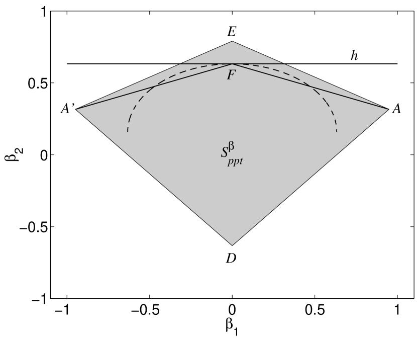
Let us now turn to the case of half-integer spins $j_{2}$, i. e., we assume that $N$ is even. Of course, we again have that $A$ and $A^{\prime}$ belong to $W^{\beta}$. But also $D\in W^{\beta}$ because the state $|j_{2},+j_{2}\rangle$ exists for integer as well as for half-integer spins $j_{2}$. The argument following Eq. (51) can thus also be applied in the present case. It follows that $S^{\beta}_{\mathrm{sep}}$ contains at least the triangle $AA^{\prime}D$ (see Fig. 3).

Figure 3: The set of PPT states $S^{\beta}_{\mathrm{ppt}}$ for $N=4$. The set $S^{\beta}_{\mathrm{sep}}$ lies entirely below the straight line $h$ through $F$ which is parallel to the $\beta_{1}$-axis. The broken line shows the curve defined by Eqs. (70) and (71).

On the other hand, the state $|j_{2},m_{2}=0\rangle$ exists, of course, only for integer spins $j_{2}$. Instead of (46) we consider the states

$$|\varphi^{(1)}\rangle=|1,0\rangle,\qquad|\varphi^{(2)}\rangle=|j_{2},+1/2\rangle,$$ (54)

which lead to

$$\tilde{\beta}_{1}=0,\qquad\tilde{\beta}_{2}=\sqrt{\frac{(N+2)(N-2)}{2(N+1)(N-1)}}.$$ (55)

This shows that the point

$$F=\left(0,\sqrt{\frac{(N+2)(N-2)}{2(N+1)(N-1)}}\right)$$ (56)

belongs to $W^{\beta}$. Hence, $S^{\beta}_{\mathrm{sep}}$ contains at least the polygon with the vertices $A$, $A^{\prime}$, $D$ and $F$.

We introduce the straight line $h$ which intersects the point $F$ and which is parallel to the $\beta_{1}$-axis (see Fig. 3). We are going to demonstrate that $S^{\beta}_{\mathrm{sep}}$ lies entirely below this line. The line $h$ is thus tangential to $S^{\beta}_{\mathrm{sep}}$ and corresponds to an optimal entanglement witness (see Sec. V). To show this we employ the rotational invariance of the functions $\tilde{\beta}_{K}$ [see Eq. (30)] to obtain a suitable parametrization of the states of the first spin $j_{1}=1$. Namely, by an appropriate rotation $R$ any state of this spin can be brought into the following form:

$$|\varphi^{(1)}\rangle=\sqrt{r}|1,+1\rangle+\sqrt{1-r}|1,-1\rangle,$$ (57)

where we omit an irrelevant overall phase factor and $r$ is a real parameter taken from the interval $[0,1]$. Invoking the rotational invariance we may assume without restriction that $|\varphi^{(1)}\rangle$ is of this form. The state space of the first spin $j_{1}$ has thus only a single relevant parameter $r\in[0,1]$.

By use of the representation (57) the quantities $\tilde{\beta}_{1}$ and $\tilde{\beta}_{2}$ become functions of the parameter $r$ and of the state vector $|\varphi^{(2)}\rangle$ of the second spin. Inserting Eq. (57) into Eq. (IV) and using Eqs. (85) and (86) of Appendix A we get

$$\tilde{\beta}_{1}[r,\varphi^{(2)}]=\sqrt{\frac{N}{2}}(2r-1)\langle\varphi^{(2)}|T^{(2)}_{10}|\varphi^{(2)}\rangle.$$ (58)

The function $\tilde{\beta}_{2}$ is found by substituting the expression (57) into Eq. (IV) and by using Eqs. (87)-(A). One finds that $\tilde{\beta}_{2}$ can be written as the expectation value

$$\tilde{\beta}_{2}[r,\varphi^{(2)}]=\langle\varphi^{(2)}|H(\lambda)|\varphi^{(2)}\rangle$$ (59)

of the Hermitian $(N\times N)$ matrix

$$H(\lambda)\equiv H_{0}+\lambda H_{1}.$$ (60)

Here, we have defined

$$H_{0}=\sqrt{\frac{N}{10}}T^{(2)}_{20},\qquad H_{1}=\frac{1}{2}\sqrt{\frac{3N}{5}}\left(T^{(2)}_{22}+T^{(2)\dagger}_{22}\right),$$

and introduced the parameter

$$\lambda=2\sqrt{r(1-r)},\qquad 0\leq\lambda\leq 1.$$ (61)

Figure 4: The largest eigenvalue $\varepsilon_{0}(\lambda)$ of the matrix $H(\lambda)$ defined by Eq. (60) for different values of $N$.

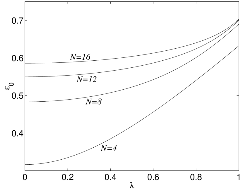
For a given value of $\lambda$ the function $\tilde{\beta}_{2}$ defined by Eq. (59) is certainly smaller than or equal to the largest eigenvalue of $H(\lambda)$ which we denote by $\varepsilon_{0}(\lambda)$. We are going to demonstrate below that $\varepsilon_{0}(\lambda)$ is a monotonically increasing function of $\lambda$ and attains its maximum at $\lambda=1$:

$$\varepsilon_{0}(1)=\sqrt{\frac{(N+2)(N-2)}{2(N+1)(N-1)}}.$$ (62)

Hence, we have

$$\tilde{\beta}_{2}[r,\varphi^{(2)}]\leq\varepsilon_{0}(1)$$ (63)

for all $r$ and $|\varphi^{(2)}\rangle$. Note that $\varepsilon_{0}(1)$ is equal to the $\beta_{2}$-coordinate of the point $F$ [see Eq. (56)]. This shows that, as claimed, all points of $W^{\beta}$ and, hence, all points of $S^{\beta}_{\mathrm{sep}}$ lie below the line $h$.

To prove that $\varepsilon_{0}(\lambda)$ is a monotonically increasing function of $\lambda$ we denote the eigenvalues of $H(\lambda)$ by $\varepsilon_{n}(\lambda)$, where $n=0,1,2\ldots$, and $n=0$ labels the largest eigenvalue. With the help of Eq. (83) one verifies that $H(\lambda)$ is invariant under time reversal. It follows that if $|\varphi\rangle$ is an eigenstate of $H(\lambda)$ then also the time reversed state $\tau|\varphi\rangle$ is an eigenstate with the same eigenvalue. Since $j_{2}$ is half-integer valued the states $|\varphi\rangle$ and $\tau|\varphi\rangle$ are orthogonal. In fact, using the antiunitarity of $\tau$ and Eq. (26) we get

$$\langle\tau\varphi|\varphi\rangle=\langle\tau^{2}\varphi|\tau\varphi\rangle^{\ast}=(-1)^{2j_{2}}\langle\tau\varphi|\varphi\rangle=-\langle\tau\varphi|\varphi\rangle,$$

which shows that $\langle\tau\varphi|\varphi\rangle=0$.

All eigenvalues $\varepsilon_{n}(\lambda)$ are thus two-fold degenerate and we write the corresponding eigenstates as $|\varphi_{n,k}(\lambda)\rangle$, where the index $k=1,2$ labels the eigenstates corresponding to the same eigenvalue: $|\varphi_{n,2}(\lambda)\rangle=\tau|\varphi_{n,1}(\lambda)\rangle$. We remark that the two-fold degeneracy is analogous to the Kramers degeneracy according to which the energy levels of an invariant system of an odd number of spin-$\frac{1}{2}$ particles are at least two-fold degenerate (see, e. g. SAKURAI ).

The Hellman-Feynman theorem now yields

$$\frac{d\varepsilon_{0}}{d\lambda}=\langle\varphi_{0,1}(\lambda)|H_{1}|\varphi_{0,1}(\lambda)\rangle.$$ (64)

In particular, we have

$$\left.\frac{d\varepsilon_{0}}{d\lambda}\right|_{\lambda=0}=0.$$ (65)

On differentiating Eq. (64) once again we find:

$$\frac{d^{2}\varepsilon_{0}}{d\lambda^{2}}=2\sum_{n\neq 0,k}\frac{|\langle\varphi_{n,k}(\lambda)|H_{1}|\varphi_{0,1}(\lambda)\rangle|^{2}}{\varepsilon_{0}(\lambda)-\varepsilon_{n}(\lambda)}\geq 0.$$ (66)

This shows that $\varepsilon_{0}(\lambda)$ is a convex function of $\lambda$ with zero derivative at $\lambda=0$. It follows that $\varepsilon_{0}(\lambda)$ increases monotonically. Some examples of the behaviour of this functions are shown in Fig. 4.

It remains to verify Eq. (62). We first note that $H(1)$ can be written with the help of Eqs. (87) and (A) in terms of the spin operator $\hat{\bm{j}}^{(2)}$ as:

$$H(1) = 2\sqrt{\frac{2}{(N+2)(N+1)(N-1)(N-2)}}$$ (67)

$$\times\left(\left[\hat{\bm{j}}^{(2)}\right]^{2}-3\left[\hat{j}_{y}^{(2)}\right]^{2}\right).$$

The largest eigenvalue of this matrix is given by

$$\varepsilon_{0}(1) = 2\sqrt{\frac{2}{(N+2)(N+1)(N-1)(N-2)}}$$ (68)

$$\times\left(j_{2}(j_{2}+1)-\frac{3}{4}\right).$$

Using $N=2j_{2}+1$ one shows that this equation coincides with Eq. (62).

We finally demonstrate that the boundary of $S^{\beta}_{\mathrm{sep}}$ is differentiable at the point $F$ [see Eq. (56)]. To this end, we construct a smooth curve which belongs to $W^{\beta}$ and passes the point $F$. Consider the following fixed state of the second spin:

$$|\varphi^{(2)}\rangle=\frac{1}{\sqrt{2}}\left|\hat{j}^{(2)}_{y}=+1/2\right\rangle+\frac{i}{\sqrt{2}}\left|\hat{j}^{(2)}_{y}=-1/2\right\rangle.$$ (69)

This is an eigenstate of the matrix $H(1)$ [Eq. (67)] corresponding to the largest eigenvalue $\varepsilon_{0}(1)$. Since $|\varphi^{(2)}\rangle$ is fixed the functions $\tilde{\beta}_{1}$ and $\tilde{\beta}_{2}$ depend only on the parameter $r$ and describe a curve in the $(\beta_{1},\beta_{2})$-plane. Writing $r\equiv(1+\mu)/2$ and determining the matrix elements one finds:

$$\tilde{\beta}_{1} = \sqrt{\frac{3N^{2}}{8(N+1)(N-1)}}\mu,$$ (70)

$$\tilde{\beta}_{2} = \frac{\varepsilon_{0}(1)}{4}\left(1+3\sqrt{1-\mu^{2}}\right),$$ (71)

where $-1\leq\mu\leq+1$. The curve described by these equations represents the upper half of an ellipse in the $(\beta_{1},\beta_{2})$-plane (see Fig. 3). It intersects the point $F$ and lies entirely in $W^{\beta}$. Since $F$ is the only point of $h$ belonging to $W^{\beta}$, it follows that the boundary of the separability region must be curved and that it is differentiable at the extreme point $F$, the line $h$ being the tangent. Summarizing, we have shown:

Theorem 2

For half-integer spins $j_{2}=\frac{3}{2},\frac{5}{2},\frac{7}{2},\ldots$ the set $S^{\beta}_{\mathrm{sep}}$ of separable states is a true subset of the set of PPT states. Hence, for all $3\otimes N$ systems with even $N$ the PPT criterion is only necessary and there always exist entangled PPT states. The line $h$ represents the tangent to $S^{\beta}_{\mathrm{sep}}$ at the extreme point $F$. The set $S^{\beta}_{\mathrm{sep}}$ is bounded by the straight lines $AD$ and $A^{\prime}D$ and by a concave curve which passes the points $A$, $A^{\prime}$ and $F$.

V Discussion and conclusions

The state space structure of rotationally invariant spin systems has been analyzed in this paper. The set of invariant states has been represented by means of two systems of invariant operators, namely by the projections $P_{J}$ onto the total angular momentum manifolds and by the invariant operators $Q_{K}$ composed of the spherical tensors. The transformation between both representations was found to be given by a matrix $L$ which is determined by certain $6$-$j$ symbols of Wigner. The $Q_{K}$-representation is particularly useful in applying the PPT criterion for separability because the $Q_{K}$ are eigenoperators of the partial time reversal. The method has been demonstrated to lead to a complete classification of separability of $3\otimes N$ systems. We have shown that the PPT criterion is necessary and sufficient for all system with odd $N$, while entangled PPT states exist for systems with even $N$.

Some remarks on the structure of the state space in the limit $N\rightarrow\infty$ might be of interest. In this limit the value of the second spin $j_{2}$ becomes arbitrary large. We infer from Eqs. (39)-(42) that the point $B$ then converges to the point $A^{\prime}$, and $C$ to $D$. At the same time $F$ converges to $E$ [see Eqs. (43) and (56)]. Hence, as $N$ increases the set $S^{\beta}_{\mathrm{ppt}}$ approaches the set $S^{\beta}$ and $S^{\beta}_{\mathrm{sep}}$ approaches $S^{\beta}_{\mathrm{ppt}}$. This behaviour is also indicated in Fig. 2. The limit $N\rightarrow\infty$ thus corresponds to a kind of classical limit in which all invariant states have a positive partial transpose and are separable.

The line $h$ constructed in Sec. IV leads to an entanglement witness which we denote by ${\mathcal{W}}$. An entanglement witness is a Hermitian operator which satisfies ${\mathrm{tr}}\{{\mathcal{W}}\sigma\}\geq 0$ for any separable state $\sigma$, and ${\mathrm{tr}}\{{\mathcal{W}}\rho\}<0$ for at least one non-separable state $\rho$ HORODECKI96a ; TERHAL . The hyperplane $h$ corresponding to an entanglement witness ${\mathcal{W}}$ is defined by ${\mathrm{tr}}\{{\mathcal{W}}\rho\}=0$. In the case of $3\otimes N$ systems $h$ is a one-dimensional line and the witness is, in fact, optimal LEWENSTEIN00 because $h$ is tangential to the region of separable states. We have formulated the witness in $\beta$-space. Transforming back to $\alpha$-space one easily shows that the entanglement witness corresponding to $h$ may be written in terms of the projections $P_{J}$ as:

$${\mathcal{W}}=-\frac{1}{N-2}P_{j_{2}-1}+P_{j_{2}}+\frac{1}{N+2}P_{j_{2}+1}.$$ (72)

This expression leads to the following physical interpretation of ${\mathcal{W}}$. Suppose one carries out a measurement of the total angular momentum $J$ on some invariant state $\rho$. If $\rho$ is separable the inequality

$$-\frac{p_{j_{2}-1}}{N-2}+p_{j_{2}}+\frac{p_{j_{2}+1}}{N+2}\geq 0$$ (73)

must be satisfied, where $p_{J}={\mathrm{tr}}\{P_{J}\rho\}$ denotes the probability of finding the value $J$. In other words, if the inequality (73) is violated the state $\rho$ must necessarily be entangled.

We exploit the witness (72) to design a prescription for the detection of entangled PPT states in $3\otimes N$ systems with even $N$ (bound entanglement HORODECKI98 ). A given state $\rho$ is positive under partial transposition if and only if the corresponding point $(\beta_{1},\beta_{2})$ lies below the line through $A^{\prime}$ and $E$, and above the line through $A^{\prime}$ and $D$ (see Fig. 1). If we transform to $\alpha$-space this yields the conditions

$$-\frac{2p_{j_{2}-1}}{N-1}+\frac{(N^{2}-5)p_{j_{2}}}{(N+1)(N-1)}+\frac{2p_{j_{2}+1}}{N+1}\geq 0$$ (74)

and

$$\frac{2p_{j_{2}-1}}{(N-1)(N-2)}-\frac{2p_{j_{2}}}{N-1}+p_{j_{2}+1}\geq 0.$$ (75)

These inequalities are equivalent to the PPT condition (27). Hence, entangled PPT states can be detected in the following way: Suppose again that a total angular momentum measurement is performed on some state $\rho$. If one finds that the measurement outcomes, i. e. the probabilities $p_{J}$, satisfy the inequalities (74) and (75) and violate the inequality (73) then the state $\rho$ must be an entangled PPT state.

The witness ${\mathcal{W}}$ defined in Eq. (72) does not detect all entangled PPT states. As has been shown in Sec. IV a part of the boundary of the region of the separable states is curved and, therefore, one needs an infinite number of linear entanglement witnesses. The upper boundary of $S^{\beta}_{\mathrm{sep}}$ can of course be described by means of a suitable nonlinear equation. A possible way to derive the latter is to construct the envelope of appropriate families of curves of the type given by Eqs. (70) and (71).

The considerations of Sec. IV reveal that for $3\otimes N_{2}$ systems half-integer spins are crucial for the emergence of entangled PPT states. The entanglement structure of systems involving half-integer spins is thus quite different from those with integer spins. It seems that this is closely connected to the fact that pure states which are invariant under time reversal only exist for integer spins, while for half-integer spins a given pure state is always orthogonal to its time reversed state. A clear physical interpretation of this result and its generalization to arbitrary $N_{1}\otimes N_{2}$ systems is of great interest. The next step to further investigate this point could be to study $4\otimes N_{2}$ systems, which is possible by the method developed in this paper.

Appendix A Spherical tensor operators

We define here the irreducible spherical tensor operators $T_{Kq}$ acting on the state space ${\mathbb{C}}^{N}$ of a particle with spin $j$, where $N=2j+1$, $K=0,1,\ldots,2j$, and $q=-K,\ldots,+K$. The tensor operators $T^{(i)}_{K_{i}q_{i}}$ for $i=1,2$ used in the main text are obtained by setting $j=j_{1}$ or $j=j_{2}$.

The spherical tensor operators $T_{Kq}$ represent a complete system of operators on ${\mathbb{C}}^{N}$. This means that any operator on the state space of the spin-$j$ particle may be written as a unique linear combination of the $T_{Kq}$. Moreover, the tensors are orthonormal with respect to the Hilbert-Schmidt inner product:

$${\mathrm{tr}}\left\{T^{\dagger}_{K^{\prime}q^{\prime}}T_{Kq}\right\}=\delta_{KK^{\prime}}\delta_{qq^{\prime}}.$$ (76)

For a fixed $K$ the $(2K+1)$ operators $T_{Kq}$ represent the spherical components of a tensor of rank $K$. They transform according to an irreducible representation of $\mathrm{SO(3)}$ which corresponds to the angular momentum $K$:

$$D^{(j)}(R)T_{Kq}D^{(j)}(R)^{\dagger}=\sum_{q^{\prime}=-K}^{+K}D^{(K)}_{q^{\prime}q}(R)T_{Kq^{\prime}}.$$ (77)

For instance, the $T_{1q}$ behave as components of a vector, and the $T_{2q}$ as components of a second-rank tensor.

The matrix elements of the tensors may be defined in term of Wigner’s $3$-$j$ symbols as WIGNER ; EDMONDS

$$\langle j,m|T_{Kq}|j,m^{\prime}\rangle=\sqrt{2K+1}(-1)^{j-m}\left(\begin{array}[]{ccc}j&j&K\\ m&-m^{\prime}&-q\end{array}\right).$$ (78)

The $3$-$j$ symbols are closely related to the Clebsch-Gordan coefficients:

$$\langle j_{1},m_{1};j_{2},m_{2}|JM\rangle=$$ (81)

$$\sqrt{2J+1}(-1)^{j_{1}-j_{2}+M}\left(\begin{array}[]{ccc}j_{1}&j_{2}&J\\ m_{1}&m_{2}&-M\end{array}\right).$$

According to the selection rules for the $3$-$j$ symbols the matrix element (78) is equal to zero for $m-m^{\prime}-q\neq 0$. In particular, we have $T_{00}=\frac{1}{\sqrt{N}}I$.

The matrix elements (78) of the tensor operators are real and one has $T^{\dagger}_{Kq}=T^{T}_{Kq}=(-1)^{q}T_{K,-q}$. It follows that the $T_{Kq}$ are eigenoperators of the time reversal transformation $\vartheta$ which was defined in Eq. (25). In fact, using the transformation behaviour (77) of the tensors and the fact that a rotation by $\pi$ about the $y$-axis is represented by the unitary matrix

$$D^{(K)}_{q^{\prime}q}(\pi)=(-1)^{K-q^{\prime}}\delta_{q^{\prime},-q},$$ (82)

one finds

$$\vartheta T_{Kq}=VT^{T}_{Kq}V^{\dagger}=(-1)^{K}T_{Kq}.$$ (83)

As a consequence the operators $Q_{K}$ which have been introduced in Eq. (7) are eigenoperators of the partial time reversal $\vartheta_{2}=I\otimes\vartheta$:

$$\vartheta_{2}Q_{K}=(-1)^{K}Q_{K}.$$ (84)

We finally list the non-vanishing matrix elements of the tensor operators needed in Sec. IV:

$$\langle j,m|T_{10}|j,m\rangle=2m\sqrt{\frac{3}{N(N-1)(N+1)}},$$ (85)

$$\langle j,m|T_{11}^{\dagger}|j,m+1\rangle=-\sqrt{\frac{6(j-m)(j+m+1)}{N(N-1)(N+1)}},$$ (86)

$$\langle j,m|T_{20}|j,m\rangle=\frac{2\sqrt{5}[3m^{2}-j(j+1)]}{\sqrt{(N+2)(N+1)N(N-1)(N-2)}},$$ (87)

$$\langle j,m|T_{21}^{\dagger}|j,m+1\rangle=$$

$$-\sqrt{5}(1+2m)\sqrt{\frac{6(j-m)(j+m+1)}{(N+2)(N+1)N(N-1)(N-2)}},$$

$$\langle j,m|T_{22}^{\dagger}|j,m+2\rangle=$$

$$\sqrt{5}\sqrt{\frac{6(j-m-1)(j-m)(j+m+1)(j+m+2)}{(N+2)(N+1)N(N-1)(N-2)}}.$$

Appendix B Proof of relation (14)

The starting point is given by Eq. (13). We insert into this equation the definitions (2) and (7) for the invariant operators $P_{J}$ and $Q_{K}$, and introduce complete sets of product basis states $|j_{1},m_{1};j_{2},m_{2}\rangle$. This yields a multiple sum over products of two Clebsch-Gordan coefficients and two matrix elements of the tensor operators. By use of Eqs. (78) and (81) the Clebsch-Gordan coefficients as well as the matrix elements of the spherical tensors can be written in terms of the $3$-$j$ symbols. We also use the selection rules for the $3$-$j$ symbols and their symmetry properties. This procedure leads to the following sum over $4$-fold products of $3$-$j$ symbols:

$$L_{KJ} = \sqrt{(2K+1)(2J+1)}(-1)^{j_{1}+j_{2}+J}\times$$

$$\sum_{\{m_{i}\}}\chi(\{m_{i}\})\times$$

$$\;\;\;\;\;\;\left(\begin{array}[]{ccc}j_{1}&j_{2}&J\\ m_{1}&m_{2}&m_{3}\end{array}\right)\left(\begin{array}[]{ccc}j_{1}&j_{1}&K\\ -m_{1}&m_{5}&-m_{6}\end{array}\right)\times$$ (95)

$$\;\;\;\;\;\;\left(\begin{array}[]{ccc}j_{2}&j_{2}&K\\ -m_{4}&-m_{2}&m_{6}\end{array}\right)\left(\begin{array}[]{ccc}j_{2}&j_{1}&J\\ m_{4}&-m_{5}&-m_{3}\end{array}\right),$$ (100)

where $\chi(\{m_{i}\})$ is a phase factor:

$$\chi(\{m_{i}\}) = (-1)^{j_{1}+m_{1}}(-1)^{j_{2}+m_{2}}(-1)^{J+m_{3}}\times$$

$$(-1)^{j_{2}+m_{4}}(-1)^{j_{1}+m_{5}}(-1)^{K+m_{6}}.$$

The sum over the quantum numbers $m_{1},\ldots,m_{6}$ in Eq. (B) exactly corresponds to a certain $6$-$j$ symbol of Wigner WIGNER . A general $6$-$j$ symbol involves six angular momenta and is written as

$$\left\{\begin{array}[]{ccc}j_{1}&j_{2}&j_{3}\\ j_{4}&j_{5}&j_{6}\end{array}\right\}.$$ (101)

The sum of Eq. (B) is equal to the $6$-$j$ symbol (101) with $j_{3}=J$, $j_{4}=j_{2}$, $j_{5}=j_{1}$ and $j_{6}=K$. Hence, we see that Eq. (B) reduces to Eq. (14). We remark that a similar technique has been used in Ref. NtensorN in order to derive an expression for the matrix which represents the partial time reversal $\vartheta_{2}$ in the $P_{J}$-representation.

By use of the formulae for the $6$-$j$ symbols EDMONDS we find that the first three rows of $L$ are given by

$$L_{0J}=\sqrt{\frac{2J+1}{N_{1}N_{2}}},$$ (102)

and

$$L_{1J}=-2\sqrt{3(2J+1)}\frac{j_{1}(j_{1}+1)+j_{2}(j_{2}+1)-J(J+1)}{\sqrt{(N_{1}-1)N_{1}(N_{1}+1)(N_{2}-1)N_{2}(N_{2}+1)}},$$ (103)

$$L_{2J}=2\sqrt{5(2J+1)}\frac{3X(X-1)-4j_{1}(j_{1}+1)j_{2}(j_{2}+1)}{\sqrt{(N_{1}-2)(N_{1}-1)N_{1}(N_{1}+1)(N_{1}+2)(N_{2}-2)(N_{2}-1)N_{2}(N_{2}+1)(N_{2}+2)}},$$ (104)

where $X\equiv j_{1}(j_{1}+1)+j_{2}(j_{2}+1)-J(J+1)$.

References

- (1) R. F. Werner, Phys. Rev. A 40, 4277 (1989).
- (2) K. Eckert, O. Gühne, F. Hulpke, P. Hyllus, J. Korbicz, J. Mompart, D. Bruß, M. Lewenstein and A. Sanpera, in Quantum Information Processing, edited by G. Leuchs and T. Beth (Wiley-VCH, Berlin, 2005).
- (3) G. Alber, T. Beth, M. Horodecki, P. Horodecki, R. Horodecki, M. Rötteler, H. Weinfurter, R. Werner and A. Zeilinger, Quantum Information (Springer-Verlag, Berlin, 2001).
- (4) M. A. Nielsen and I. L. Chuang, Quantum Computation and Quantum Information (Cambridge University Press, Cambridge, 2000).
- (5) A. Peres, Phys. Rev. Lett. 77, 1413 (1996).
- (6) M. Horodecki, P. Horodecki and R. Horodecki, Phys. Lett. A 223, 1 (1996).
- (7) M. Horodecki and P. Horodecki, Phys. Rev. A 59, 4206 (1999).
- (8) N. J. Cerf, C. Adami and R. M. Gingrich, Phys. Rev. A 60, 898 (1999).
- (9) M. A. Nielsen and J. Kempe, Phys. Rev. Lett. 86, 5184 (2001).
- (10) O. Rudolph, Phys. Rev. A 67, 032312 (2003).
- (11) Kai Chen and Ling-An Wu, Quant. Inf. Comp. 3, 193 (2003).
- (12) B. M. Terhal, Phys. Lett. A 271, 319 (2000).
- (13) M. Lewenstein, B. Kraus, J. I. Cirac and P. Horodecki, Phys. Rev. A 62, 052310 (2000).
- (14) E. M. Rains, Phys. Rev. A 60, 179 (1999).
- (15) K. G. H. Vollbrecht and R. F. Werner, Phys. Rev. A 64, 062307 (2001).
- (16) H. P. Breuer and F. Petruccione, The Theory of Open Quantum Systems (Oxford University Press, Oxford, 2002).
- (17) M. Verri and V. Gorini, J. Math. Phys. 19, 1803 (1978).
- (18) A. Osterloh, L. Amico, G. Falci and R. Fazio, Nature 416, 608 (2002).
- (19) T. J. Osborne and M. A. Nielsen, Phys. Rev. A 66, 032110 (2002).
- (20) G. A. Durkin, C. Simon, J. Eisert and D. Bouwmeester, Phys. Rev. A 70, 062305 (2004).
- (21) K. K. Manne, C. M. Caves, e-print eprint quant-ph/0506151.
- (22) J. Schliemann, J. I. Cirac, M. Kuś, M. Lewenstein and D. Loss, Phys. Rev. A 64, 022303 (2001).
- (23) K. Eckert, J. Schliemann, D. Bruß and M. Lewenstein, Ann. Phys. (N.Y.) 299, 88 (2002).
- (24) J. Schliemann, Phys. Rev. A 68, 012309 (2003).
- (25) H. P. Breuer, e-print eprint quant-ph/0503079 (Phys. Rev. A, in press).
- (26) J. Schliemann, e-print eprint quant-ph/0503123 (Phys. Rev. A, in press).
- (27) B. Hendriks, Diploma thesis, University of Braunschweig, Germany, 2002.
- (28) A. R. Edmonds, Angular Momentum in Quantum Mechanics (Princeton University Press, Princeton, 1957).
- (29) J. Schwinger, in Quantum Theory of Angular Momentum, edited by L. C. Biedenharn and H. Van Dam (Academic Press, New York, 1965), p. 229.
- (30) E. P. Wigner, Group theory and its application to the quantum mechanics of atomic spectra (Academic Press, New York, 1959).
- (31) J. J. Sakurai, Modern Quantum Mechanics (Addison-Wesley Publishing Company, Reading, 1994).
- (32) M. Horodecki, P. Horodecki and R. Horodecki, Phys. Rev. Lett. 80, 5239 (1998).