Noncyclic Pancharatnam phase for mixed state SU(2) evolution
in neutron polarimetry

Abstract

We have measured the Pancharatnam relative phase for spin-1/2 states. In a neutron polarimetry experiment the minima and maxima of intensity modulations, giving the Pancharatnam phase, were determined. We also considered general SU(2) evolution for mixed states. The results are in good agreement with theory.

I Introduction

In recent years much attention has been paid to the concept of geometric phase. Since its discovery by Berry Berry1984 the subject was widely expanded and subdued to several generalizations ShapereWilczek1989 , e.g. non adiabatic AharanovAnandan1987 and noncyclic SamuelBhandari1988 evolutions as well as the off-diagonal case ManiniPistolesi2000 . Ever since, a great variety of experimental confirmations of the Berry phase and its peculiar properties have been accomplished (see e.g. TomitaChao1986 ; WeinfurterBadurek1990 ; BadurekEtAl1993 ; AllmanEtAl1997 ; HasegawaEtAl2001 ; HasegawaEtAl2003 ). In 1956 Pancharatnam defined $\phi=\mbox{arg}\langle\psi_{0}|\psi\rangle$ as the phase acquired during an entirely arbitrary evolution of a wave-function Pancharatnam1956 . Provided the evolution takes place under condition of parallel transport, $\phi$ can be identified with the noncyclic geometric phase. Quite recently, also a concept of mixed state phase was developed by Sjöqvist et al. SjoeqvistEtAl2000 due to its importance in quantum computation. The theoretical predictions have been tested by Du et al. DuEtAl2003 and Ericsson et al. EricssonEtAl2004 using NMR and single-photon interferometry, respectively. In this letter, we report a neutron polarimetry experiment for measuring the Pancharatnam relative phase of a spinor subdued to an arbitrary SU(2) evolution, implementing the method described by Wagh and Rakhecha in WaghRakhecha1995 . We test its extension to the mixed state case put forward by Larsson and Sjöqvist LarssonSjoeqvist2003 .

II The pure state case

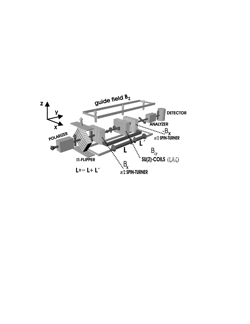
Figure 1: Sketch of the neutron polarimetry setup for Pancharatnam phase measurement including evolution of polarization vector for one specific relative position of spin turners at distance L₀ and SU(2) coils.

We consider the experimental setup shown in Fig. 1. A monochromatized neutron beam, polarized along the $+z$ direction experiences a $\pi$/2 flip about the $x$-axis, therefore being denoted as a superposition of the orthogonal states $|\pm z\rangle$. The beam travels in an overall guide field B_z of the length L, which is chosen to be parallel to the $+z$ direction. Under the influence of B_z the polarization vector rotates through an angle $\eta$ determined by the distance L. The two orthogonal components $|\pm z\rangle$ of the rotated superposition state acquire opposite phase undergoing the SU(2) transformation $\hat{\mbox{U}}_{0}$, denoted by the matrix

$$\mbox{U}_{0}(\xi,\delta,\zeta) = \left(\begin{array}[]{cc}\mbox{e}^{i\delta}\cos\xi&~{}-\mbox{e}^{-i\zeta}\sin\xi\\ \mbox{e}^{i\zeta}\sin\xi&~{}\mbox{e}^{-i\delta}\cos\xi\end{array}\right).$$ (3)

In neutron polarimetry the unitary, unimodular operator $\hat{\mbox{U}}(\vec{\alpha})$ is used for description of spin rotations (transformations) carried out within magnetic fields. By comparison of Eq.(3) to the matrix representation of $\hat{\mbox{U}}(\vec{\alpha})$, with

$$\hat{\mbox{U}}(\vec{\alpha}) = \exp\left(-i\frac{\hat{\vec{\sigma}}\cdot\vec{\alpha}}{2}\right)$$ (4)

$$= \hat{\mathchoice{\rm 1\mskip-4.2mul}{\rm 1\mskip-4.2mul}{\rm 1\mskip-4.6mul}{\rm 1\mskip-5.2mul}}\cos\frac{\alpha}{2}-i\left(\hat{\vec{\sigma}}\cdot\frac{\vec{\alpha}}{\alpha}\right)\sin\frac{\alpha}{2},$$

one is lead to sets ($\xi,\delta,\zeta$) of SU(2) parameters. $\vec{\alpha}$ points to the direction of the magnetic field constituting the rotation axis and $|\vec{\alpha}|=\alpha$ denotes the rotation angle. $\hat{\vec{\sigma}}$ is the Pauli vector operator. The resulting beam passes a distance L’ along the guide field B_z, its polarization rotating through the associated angle $2\mbox{n}\pi-\eta$ (n$=1,2,...$). L${}_{0}=$ L$+$L’ is set in such a way that the accumulated rotation angle within B_z equals an integer multiple of $2\pi$, $\mbox{L}_{0}=\mbox{n}\pi\hbar\mbox{v}/|\mu\mbox{B}_{z}|$. Finally, a $-\pi$/2 flip around the $x$-axis is applied and the output intensity, calculated as

I $$= \cos^{2}\xi\cos^{2}\delta+\sin^{2}\xi\sin^{2}(\zeta+\eta)$$ (5)

for the pure state case, is measured. The phase shift $\eta$, implemented by variation of the distances L and L’ at constant L₀ causes intensity modulations, yielding the extreme values

$$\mbox{I}_{\mbox{\scriptsize min}} = \cos^{2}\xi\cos^{2}\delta,$$ (6)

$$\mbox{I}_{\mbox{\scriptsize max}} = \cos^{2}\xi\cos^{2}\delta+\sin^{2}\xi.$$ (7)

In our case, the Pancharatnam phase $\phi$ is given by substituting $|\psi_{0}\rangle$ by $|+z\rangle$ and $|\psi\rangle$ by $\hat{\mbox{U}}_{0}|+z\rangle$. The relative phase shift between $|+z\rangle$ and $\hat{\mbox{U}}_{0}|+z\rangle$, $\phi=\mbox{arg}\langle+z|\hat{\mbox{U}}_{0}|+z\rangle=\delta+\mbox{arg}\cos\xi$ for the pure state case, is therefore computed from

$$\phi = \arccos\sqrt{\frac{\mbox{I}_{\mbox{\scriptsize min}}}{1-\mbox{I}_{\mbox{\scriptsize max}}+\mbox{I}_{\mbox{\scriptsize min}}}}.$$ (8)

III The mixed state case

More general, a neutron beam passing the setup explained above at any arbitrary degree of polarization r along the positive $z$-axis is described by the density operator

$$\hat{\rho} = \frac{1}{2}(\hat{\mathchoice{\rm 1\mskip-4.2mul}{\rm 1\mskip-4.2mul}{\rm 1\mskip-4.6mul}{\rm 1\mskip-5.2mul}}+r\hat{\sigma}_{z}),$$ (9)

with the Pauli spin operator $\hat{\sigma}_{z}$ and $0\leq r\leq 1$. The measured intensity for this mixed state is given by

$$\mbox{I}^{\rho} = \frac{1-r}{2}+r\mbox{I},$$ (10)

which obviously reduces to Eq.(5) for $r=1$. The relative mixed state phase $\Phi$ SjoeqvistEtAl2000 is

$$\Phi = \arctan[r\tan(\delta+\arg\cos\xi)].$$ (11)

With the associated extreme values of Eq.(10) for $r\geq 0$,

$$\mbox{I}^{\rho}_{\mbox{\scriptsize min}} = \frac{1-r}{2}+r\cos^{2}\xi\cos^{2}\delta$$ (12)

$$\mbox{I}^{\rho}_{\mbox{\scriptsize max}} = \frac{1-r}{2}+r(\cos^{2}\xi\cos^{2}\delta+\sin^{2}\xi),$$ (13)

one obtains the following expression for the mixed state relative phase LarssonSjoeqvist2003 :

$$\Phi = \arccos\sqrt{\frac{\mbox{I}^{\rho}_{\mbox{\scriptsize min}}-1/2(1-r)}{r^{2}[1/2(1+r)-\mbox{I}^{\rho}_{\mbox{\scriptsize max}}]+\mbox{I}^{\rho}_{\mbox{\scriptsize min}}-1/2(1-r)}}.$$ (14)

This formula is consistent with the pure state case since for $r=1$ it reduces to Eq.(8). The density operator formalism is subject to an ambiguity, in a sense that certain inherently distinct physical situations are described by identical density matrices. This is often referred to as ’decomposition freedom’ (see e.g. KultSjoeqvist2004 ). Moreover, it is not apparent from Eq.(9) by what means some mixed state of the system should be produced. Considering this, we introduced a $\pi$ flip in front of the actual setup, resulting in a beam polarized in the $-z$ direction. The intensities I${}_{\mbox{\scriptsize off}}$ and I${}_{\mbox{\scriptsize on}}$, corresponding to ’spin flipper off’ and ’spin flipper on’, respectively, were measured for equal time intervals. A density matrix was calculated from a weighted sum of I${}_{\mbox{\scriptsize off}}$ and I${}_{\mbox{\scriptsize on}}$ referring to a certain degree of polarization $r\geq 0$ and is therefore equivalent to the associated mixed state. Since a real polarizer does not work perfectly, it is important to note that the incident neutron beam can already be considered to be in a mixed state, as it was done in this work. For many experiments, in contrast, it is sufficient to assume the incident beam to be purely polarized in some arbitrarily chosen direction.

IV Experiment

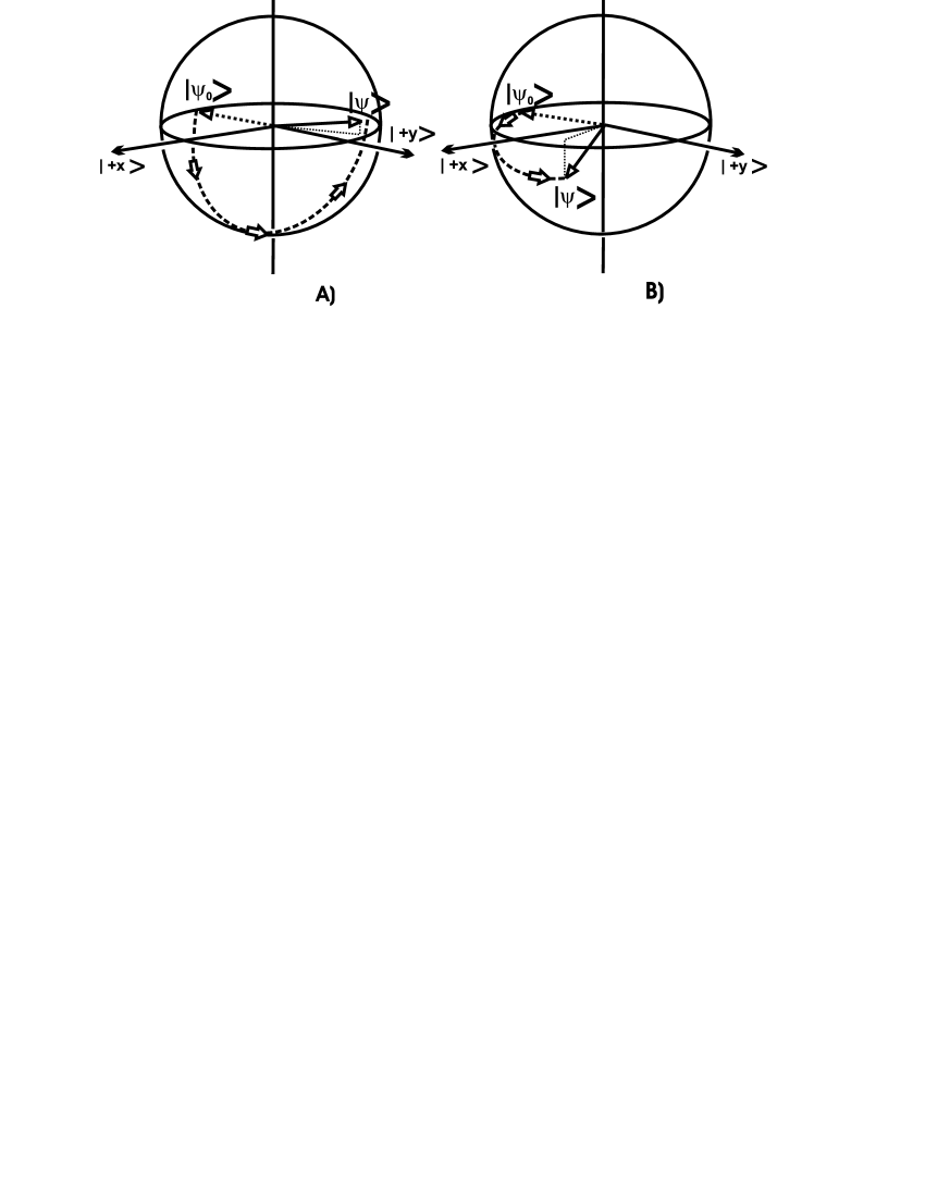
Figure 2: Rotations on the Poincaré sphere associated to parameter sets A: $(\xi^{\mbox{\scriptsize(A)}},\delta^{\mbox{\scriptsize(A)}},\zeta^{\mbox{\scriptsize(A)}})\rightarrow(1.71,0.38,-1.46)$ rad and B: $(\xi^{\mbox{\scriptsize(B)}},\delta^{\mbox{\scriptsize(B)}},\zeta^{\mbox{\scriptsize(B)}})\rightarrow(1.06,0.17,-1.40)$ rad for one specific relative position of spin turners and SU(2) coils.

The experiment was carried out at the tangential beam port of the 250 kW TRIGA research reactor of the Atomic Institute of the Austrian Universities, Vienna. The neutron beam of mean wavelength $\lambda=1.99$ Å , incident from a pyrolytic graphite monochromator, was polarized along the $+z$ direction by reflection from a bent Co-Ti supermirror array. All spin rotations were implemented by Larmor precessions about the magnetic field axes of DC coils made of anodized aluminium wire wound on frames with rectangular profile. After passing the DC $\pi$ flipper the beam encounters the first $\pi/2$ spin turner creating a superposition of the orthogonal states $|\pm z\rangle$. The polarization vector precesses in the $xy$-plane through the angle $\eta$ around the $+z$ direction in the guide field B_z and length L at an angular frequency $\omega=\frac{2\mu}{\hbar}\mbox{B}_{z}$. The guide field of length L₀ was realized by two rectangular coils of 150 cm length along the beam trajectory and a width of 12 cm. They were arranged in Helmholtz geometry to provide for optimal homogeneity. The combination of the guide field B_z measured by a Hall probe ($=5.893\pm 0.022$ G) and the distance 4 L₀ (about 46 cm) was chosen in such a way that more than one period ($\eta>2\pi$) of intensity oscillations could be scanned for its extreme values. The subsequent SU(2) transformation $\mbox{U}_{0}(\xi,\delta,\zeta)$ was carried out by two coils with mutually orthogonal orientation wound on the same frame. They define an arbitrary magnetic field axis in the $xz$-plane, whose effect on the spin state is denoted by Eq.(4). Along the distance L’ from the SU(2) coils to the second spin turner the polarization vector precesses by an angle $2\mbox{n}\pi-\eta$ about the guide field B_z before being turned through $-\pi/2$ about the $x$-axis, analyzed in the $+z$ direction by a second supermirror array and finally counted by a ³He detector. The variation of the phase shift $\eta$ is implemented by physical translation of the two $\pi/2$ spin turners at constant distance L${}_{0}=$ L $+$ L’. This can be done conveniently by steps of some mm, exhibiting the intensity oscillations evoked by the phase shift $\eta$.

Here, we present the results for two settings of SU(2) coil currents. For each set of transformation parameters ($\xi,\delta,\zeta$), three minima and maxima of $\mbox{I}_{\mbox{\scriptsize off}}$ and $\mbox{I}_{\mbox{\scriptsize on}}$ were measured in one scan. Given uncertainties contain both systematic and statistical errors.

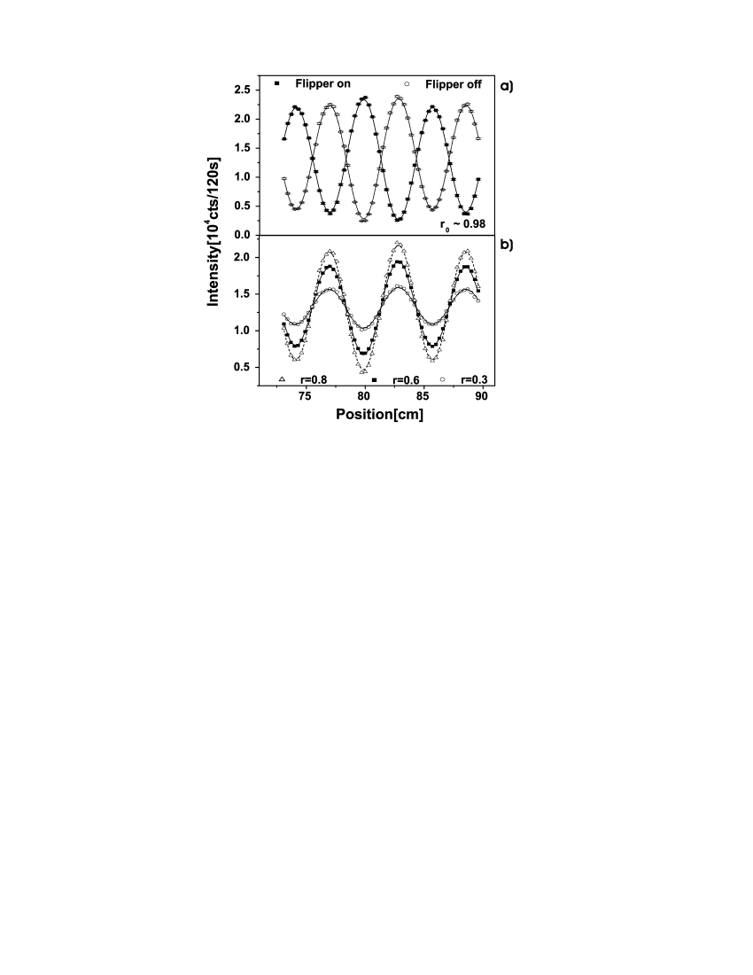
Figure 3: a) Measured intensities $\mbox{I}_{\mbox{\scriptsize off}}$ and $\mbox{I}_{\mbox{\scriptsize on}}$ for the parameter set $(\xi^{\mbox{\scriptsize(A)}},\delta^{\mbox{\scriptsize(A)}},\zeta^{\mbox{\scriptsize(A)}})\rightarrow(1.71,0.38,-1.46)$ rad at $r_{0}\sim 0.98$. b) Calculated mixed state intensities for three degrees of polarization r. Second order fits (see text) are included.

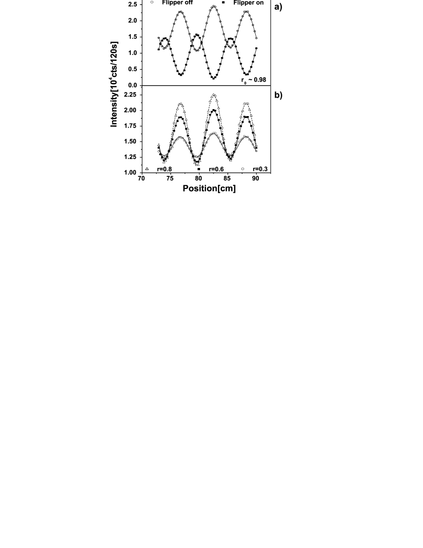
Figure 4: a) Measured intensities $\mbox{I}_{\mbox{\scriptsize off}}$ and $\mbox{I}_{\mbox{\scriptsize on}}$ for the parameter set $(\xi^{\mbox{\scriptsize(B)}},\delta^{\mbox{\scriptsize(B)}},\zeta^{\mbox{\scriptsize(B)}})\rightarrow(1.06,0.17,-1.40)$ rad at $r_{0}\sim 0.98$. b) Calculated mixed state intensities for three degrees of polarization r. Second order fits (see text) are included.

The first example is a rotation as depicted schematically in Fig. 2A. The associated SU(2) parameter set is $(\xi^{\mbox{\scriptsize(A)}},\delta^{\mbox{\scriptsize(A)}},\zeta^{\mbox{\scriptsize(A)}})\rightarrow(1.71,0.38,-1.46)$ rad. By application of Eq.(11) one obtains the theoretical result $\Phi_{\mbox{\scriptsize th}}^{\mbox{\scriptsize(A)}}=0.37$ rad, whereas the value computed from the measured data using Eq.(14) is $\Phi_{\mbox{\scriptsize m}}^{\mbox{\scriptsize(A)}}=0.38\pm 0.08$ rad at initial polarization $r^{\mbox{\scriptsize(A)}}_{0}=0.976\pm 0.004$. The measured intensities $\mbox{I}_{\mbox{\scriptsize off}}$, $\mbox{I}_{\mbox{\scriptsize on}}$ and the calculated mixed state intensities for three different degrees of polarization are shown in Fig. 3a and b, respectively. The second example is depicted in Fig. 2B, being described by parameters $(\xi^{\mbox{\scriptsize(B)}},\delta^{\mbox{\scriptsize(B)}},\zeta^{\mbox{\scriptsize(B)}})\rightarrow(1.06,0.17,-1.40)$ rad. For this set the theoretical prediction is $\Phi_{\mbox{\scriptsize th}}^{\mbox{\scriptsize(B)}}=0.17$ rad. The experimental result is $\Phi_{\mbox{\scriptsize m}}^{\mbox{\scriptsize(B)}}=0.16\pm 0.06$ rad at initial polarization $r^{\mbox{\scriptsize(B)}}_{0}=0.981\pm 0.005$. Measured and calculated intensities are shown in Fig. 4a and b. For the density matrices derived from the experimental data the results are $\Phi^{\mbox{\scriptsize(A)}}_{0.8}=0.35\pm 0.06~{}(0.31)$ rad, $\Phi^{\mbox{\scriptsize(A)}}_{0.6}=0.21\pm 0.06~{}(0.24)$ rad, $\Phi^{\mbox{\scriptsize(A)}}_{0.3}=0.05\pm 0.07~{}(0.12)$ rad for the transformation $(\xi^{\mbox{\scriptsize(A)}},\delta^{\mbox{\scriptsize(A)}},\zeta^{\mbox{\scriptsize(A)}})$ and $\Phi^{\mbox{\scriptsize(B)}}_{0.8}=0.12\pm 0.06~{}(0.14)$ rad, $\Phi^{\mbox{\scriptsize(B)}}_{0.6}=0.10\pm 0.07~{}(0.10)$ rad, $\Phi^{\mbox{\scriptsize(B)}}_{0.3}=0.02\pm 0.08~{}(0.05)$ rad for $(\xi^{\mbox{\scriptsize(B)}},\delta^{\mbox{\scriptsize(B)}},\zeta^{\mbox{\scriptsize(B)}})$. The values in parenthesis are the corresponding theoretical predictions for $\Phi$ calculated from Eq.(11).

V Discussion

The extreme values of the intensity modulations show slight irregularities in height as can be seen in the graphs. This can be explained as an effect of second order neutrons (wavelength $\lambda$/2). The monochromatization of the beam is governed by the Bragg condition $2\mbox{d}\sin\theta_{\mbox{\scriptsize B}}=\mbox{n}\lambda$, that - for a certain angle $\theta_{\mbox{\scriptsize B}}$ - is fulfilled for n$=1,2,...$ . Consequently, the beam used for the experiment is contaminated by a percentage of neutrons with only half the intended wavelength. In a time of flight (TOF) measurement, this percentage was found to be $\lesssim$ 7.2 % of the overall intensity. Neutrons that travel at double velocity spend only half the time in magnetic fields along the beam trajectory. Therefore, their spin rotates through only half the originally intended angles, showing a behavior rather different from the first order intensity. To compute the relative phase, values for $\mbox{I}_{\mbox{\scriptsize max}}$ and $\mbox{I}_{\mbox{\scriptsize min}}$ were determined from a least-squares fitting model (also shown in Fig. 3 and Fig. 4), taking into account the second order neutrons. The careful reader will point out that randomness is missing in the mixing procedure described above: the relative frequencies for finding the system in either one of the pure states $|+z\rangle$ or $|-z\rangle$ are not only well known, but even determined by the experimenter. As a matter of fact, the actual system, the neutron beam, is at no time of the experiment in one of the mixed states associated with r=0.8, 0.6 or 0.3. We are aware of the fact that the procedure carried out does by no means constitute a general mixing method, but represents a special approach within the wide scope of possible and accepted techniques for mixed state preparation. Nevertheless, the density matrices are generated by using the measured data resulting from the conducted experiments, fulfilling the predictions developed by Larsson and Sjöqvist LarssonSjoeqvist2003 . A neutron optical experiment showing the r dependence of the phase by application of some other preparation method will be carried out in the future.

The obtained experimental results are in good agreement with theoretical predictions for the relative mixed state phase, although systematic errors occur due to inherent difficulties of the experiment. Even though the guide field was constructed carefully, some inhomogeneity ($\sim 0.4$%) along its length cannot be avoided completely, accumulating an error of $\sim 5^{\circ}$ in the angle $\eta$ along the distance 4 L₀. Furthermore, it was difficult to compute values for the readjustment of 4 L₀ after a change of SU(2) coil currents. Consequently, the correct distance between the spin turners was tuned by its variation at minimum intensity relative position of spin turners and SU(2) coils, thereby exhibiting the maximum of visibility. Another point is that the two $\pi/2$ spin turners were situated within the guide field. Therefore they did not exactly carry out the designated rotations of the polarization vector to the -y direction and back to the +z direction. These inaccuracies are intrinsic to this experiment and can hardly be avoided at considerable effort. Further discussions gave rise to interesting ideas for possible improvements of the experimental setup concerning accuracy and robustness. At present, they are tested and will be described in a forthcoming paper Sponar .

VI Conclusion

To summarize, we have measured the Pancharatnam relative phase for the mixed state case in a neutron polarimetry experiment. The dependence of the phase of the degree of polarization was indicated by calculation of weighted sums of the density matrices corresponding to the measured intensities. The experimental data is in good agreement with theory. Deviations of the predicted behavior were explained to arise due to contamination of the beam by second order neutrons.

References

- (1) M.V.Berry, Proc. R. Soc. Lond. A 392, 45 (1984).
- (2) Edited by Alfred Shapere, Frank Wilczek, Geometric Phases in Physics, Advanced Series in Mathematical Physics, Vol. 5, World Scientific, 1989.
- (3) Y.Aharonov, J.S.Anandan, Phys. Rev. Lett. 58, 1593 (1987).
- (4) J.Samuel, R.Bhandari, Phys. Rev. Lett. 60, 2339 (1988).
- (5) N.Manini, F.Pistolesi, Phys. Rev. Lett. 85, 3076 (2000).
- (6) A.Tomita, R.Y.Chiao, Phys. Rev. Lett. 57, 937 (1986).
- (7) H.Weinfurter, G.Badurek, Phys. Rev. Lett. 64, 1318 (1990).
- (8) G.Badurek et al., Phys. Rev. Lett. 71, 307 (1993).
- (9) B.E.Allman et al., Phys. Rev. A 56, 4420 (1997).
- (10) Y.Hasegawa et al., Phys. Rev. Lett. 87, 070401 (2001).
- (11) Y.Hasegawa et al., Phys. Rev. A 65, 052111-1 (2002).
- (12) Pancharatnam, Proc. Indian Acad. Sci. A 44 (1956).
- (13) E.Sjöqvist et al., Phys. Rev. Lett. 85, 2845 (2000).
- (14) J.Du et al., Phys. Rev. Lett. 91, 100403 (2003).
- (15) M.Ericsson et al., Phys. Rev. Lett. 94, 050401 (2005).
- (16) A.G.Wagh, V.C.Rakhecha, Phys. Lett. A 197, 112 (1995).
- (17) P.Larsson and E.Sjöqvist, Phys. Lett. A 315, 12 (2003).
- (18) D. Kult and E.Sjöqvist, Int. J. Quantum Inf. 2, 247 (2004).
- (19) S.Sponar, J.Klepp, Y.Hasegawa, E.Jericha and G.Badurek, in preparation.