Multimode entanglement and telecloning in a noisy environment

Abstract

We address generation, propagation and application of multipartite continuous variable entanglement in a noisy environment. In particular, we focus our attention on the multimode entangled states achievable by second order nonlinear crystals, i.e. coherent states of ${\rm SU}(m,1)$ group, which provide a generalization of the twin-beam state of a bipartite system. The full inseparability in the ideal case is shown, whereas thresholds for separability are given for the tripartite case in the presence of noise. We find that entanglement of tripartite states is robust against thermal noise, both in the generation process and during propagation. We then consider coherent states of ${\rm SU}(m,1)$ as a resource for multipartite distribution of quantum information, and analyze a specific protocol for telecloning, proving its optimality in the case of symmetric cloning of pure Gaussian states. We show that the proposed protocol also provides the first example of a completely asymmetric $1\rightarrow m$ telecloning, and derive explicitly the optimal relation among the different fidelities of the $m$ clones. The effect of noise in the various stages of the protocol is taken into account, and the fidelities of the clones are analytically obtained as a function of the noise parameters. In turn, this permits the optimization of the telecloning protocol, including its adaptive modifications to the noisy environment. In the optimized scheme the clones’ fidelity remains maximal even in the presence of losses (in the absence of thermal noise), for propagation times that diverge as the number of modes increases. In the optimization procedure the prominent rule played by the location of the entanglement source is analyzed in details. Our results indicate that, when only losses are present, telecloning is a more effective way to distribute quantum information then direct transmission followed by local cloning.

I Introduction

Entanglement plays a fundamental role in quantum information, being recognized as the essential resource for quantum computing, teleportation, and cryptographic protocols. In the framework of quantum information with continuous variables (CV) vLB_rev ; Napoli the possibility of generating and manipulating entanglement allowed the realization of a variety of quantum protocols, such as teleportation, cryptography, dense coding and entanglement swapping. In these protocols the source of entanglement is the bipartite twin-beam state of two modes of radiation, usually generated by parametric down-conversion in $\chi^{(2)}$ crystals. However, recent experimental progresses Exps show that the coherent manipulation of entanglement between more then two modes may be achieved with current technology. This opens the opportunity to realize a true quantum information network, in which the information can be stored, manipulated and distributed among many parties, in a fashion resembling the current classical telecommunication networks. In a realistic implementation, entanglement needs to be transmitted along physical channels, such as optical fibers or the atmosphere. As a matter of fact, the propagation and the influence of the environment unavoidably lead to degradation of entanglement, owing to decoherence effects induced by losses and thermal noise. In this scenario, it is worth to study the entanglement properties and the possible applications of multipartite systems in noisy environments, which will be the subject of this paper.

A prominent class of CV states is constituted by the Gaussian states. They can be theoretically characterized in a convenient way, and generated and manipulated experimentally in a variety of physical systems. In a quantum information setting, entangled Gaussian states provide the basis for the quantum information protocols mentioned above. The basic reason for this is that the QED vacuum and radiation states at thermal equilibrium are themselves Gaussian states. This observation, in combination with the fact that the evolutions achievable with current technology are described by Hamiltonian operators at most bilinear in the fields, accounts for the fact that the states commonly produced in labs are Gaussian. Indeed, bilinear evolutions preserve the Gaussian character. As we already mentioned, the outmost used source of CV entanglement are the twin-beams, which belong to the class of bipartite Gaussian states. In a group-algebraic language, they are the coherent states of the group ${\rm SU}(1,1)$, i.e., the states evolved from vacuum via a unitary realization of the group. Within the class of Gaussian states, the simplest generalization of twin-beams to more then two modes are the coherent states of the group ${\rm SU}(m,1)$. Indeed, this states can be generated by multimode parametric processes in second order nonlinear crystals, with Hamiltonians that are at most bilinear in the fields. In particular, these processes involve $m+1$ modes of the field $a_{0},a_{1},\dots,a_{m}$, with mode $a_{0}$ that interacts through a parametric-amplifier-like Hamiltonian with the other modes, whereas the latter interact one each other only via a beam-splitter-like Hamiltonian vecchio ; puri . In the framework of CV quantum information, the first proposal to produce such states has been given in Ref. vLB_tlc , where a half of a two-mode squeezed vacuum state interacts with $m$ vacua via a proper sequence of beam splitters. Other unitary realizations of the algebra of ${\rm SU}(m,1)$ have been proposed, in optical settings como ; chirkin as well as with cold atoms nics or optomechanical systems cams . In these schemes the Hamiltonian of the system, rather then involving a sequence of two-mode interaction, is realized via simultaneous multimode interactions. Experimental realizations of tripartite entanglement in the optical domain have been recently reported Exps .

In this work we do not focus on any specific implementation of the ${\rm SU}(m,1)$ evolution. Rather, we will analyze the entanglement properties of ${\rm SU}(m,1)$ coherent states in a unified fashion valid for a generic Hamiltonian of this kind. As we will see in Sec. II, this is allowed by the observation that the coherent states of ${\rm SU}(m,1)$ have a common structure, which can be conveniently written in the Fock representation of the field puri . In particular, the degradation effects of both the thermal background in the generation process and of losses and thermal photons in the propagation will be outlined. The robustness of these states against noise will be analyzed in Sec. III where it will be also compared with the bipartite case.

As already mentioned, one of the main results in CV quantum communication concerned the realization of the teleportation protocol (for a recent experiment see furu05 ). The natural generalization of standard teleportation to many parties corresponds to a telecloning protocol murao . Teleportation is based on the coherent states of ${\rm SU}(1,1)$, which provide the shared entangled states supporting the protocol. Thus, in order to implement a multipartite version of this protocol, one is naturally led to consider a shared entangled state produced by a generic ${\rm SU}(m,1)$ interaction. The telecloning protocol will be analyzed in detail in Sec. IV. As concern cloning with CV, there are general results to assess the optimality of $n\rightarrow m$ symmetric cloning of coherent states cerf . Optimal local unitary realization of such schemes have been proposed in braunetal ; fiurasek , and an experimental realization of $1\rightarrow 2$ cloning has been recently reported leuchs . Concerning telecloning, existing proposals are about optimal $1\rightarrow m$ symmetric cloning of pure Gaussian states, using a particular coherent state of ${\rm SU}(m,1)$ as support vLB_tlc . Recently, a proposal which make use of partially disembodied transport has also been reported zhang . In view of the realization of a quantum information network, one is naturally led to consider the possibility to retrieve different amount of information from different clones. This means that one may consider the possibility to produce clones different one from each other, in what is called asymmetric cloning. Examples of optimal $1\rightarrow 2$ asymmetric cloning are given in Ref. fiurasek ; josab , where local and non-local realizations are considered. In this work, we will see how the telecloning protocol involving a generic coherent state of ${\rm SU}(m,1)$ provides the first example of a completely asymmetric $1\rightarrow m$ cloning of pure Gaussian states. In this sense, we provide a generalization of the proposal in Ref. vLB_tlc to the asymmetric case. Moreover, we found an expression for the maximum fidelity achievable by one clone when the fidelities of the others are fixed to prescribed values, thus giving explicitly the trade-off between the qualities of the different clones.

In Sec. V we will analyze the effect of noise in each step of the telecloning protocol. As expected, the presence of both thermal noise and losses unavoidably leads to a degradation of the cloning performances. Nevertheless, we will show that the protocol can be optimized in order to reduce these degradation effects. In particular, one may optimize not only the energy of the entangled support, but also the location of the source of entanglement itself. Remarkably, when only losses are considered, this optimization completely cancels the degrading effects of noise on the fidelity of the clones. This happens for finite propagation times which, however, diverge as the number of modes increases.

We conclude the paper with Sec. VI, where the main results will be summarized.

II Multimode parametric interactions: ${\rm\bf SU}\boldsymbol{(m,1)}$ coherent states

Let us consider the set of bilinear Hamiltonians expressed by

$$H_{m}=\sum_{l<k=1}^{m}\gamma_{kl}^{(1)}\,a_{k}a^{{\dagger}}_{l}+\sum_{k=1}^{m}\gamma_{k}^{(2)}\,a_{k}a_{0}+h.c.\;,$$ (1)

where $[a_{k},a_{l}]=0$, $[a_{k},a^{\dagger}_{l}]=\delta_{k,l}$ ($k,l=0,\dots,m$) are independent bosonic modes. A conserved quantity is the difference $D$ between the total mean photon number of the mode $a_{0}$ and the remaining modes, in formula

$$D=\sum_{k=1}^{m}a^{\dagger}_{k}a_{k}-a_{0}^{\dagger}a_{0}\;.$$ (2)

The transformations induced by Hamiltonians (1) correspond to the unitary representation of the ${\rm SU}(m,1)$ algebra puri . Therefore, the set of states obtained from the vacuum coincides with the set of ${\rm SU}(m,1)$ coherent states i.e.

$$|\boldsymbol{\Psi}_{m}\rangle\equiv\exp\left\{-iH_{m}t\right\}|\boldsymbol{0}\rangle=\exp\left\{\sum_{k=1}^{m}\beta_{k}a_{k}^{\dagger}a_{0}^{\dagger}-h.c.\right\}|\boldsymbol{0}\rangle\;,$$ (3)

where $\beta_{k}$ are complex numbers, parameterizing the state, which are related to the coupling constants $\gamma_{kl}^{(1)}$ and $\gamma_{k}^{(2)}$ in Eq. (1). Upon defining

$${\cal C}_{k}=\beta_{k}\frac{\tanh\left(\sum_{r=1}^{m}|\beta_{r}|^{2}\right)}{\sum_{r=1}^{m}|\beta_{r}|^{2}}\>,$$

$|\boldsymbol{\Psi}_{m}\rangle$ in Eq. (3) can be explicitly written as

$$|\boldsymbol{\Psi}_{m}\rangle= \sqrt{{\cal Z}_{m}}\sum_{\{\boldsymbol{n}\}}\frac{{\cal C}_{1}^{n_{1}}{\cal C}_{2}^{n_{2}}...{\cal C}_{m}^{n_{m}}\>\sqrt{(n_{1}+n_{2}+...+n_{m})!}}{\sqrt{n_{1}!n_{2}!...n_{m}!}}\>|\sum_{k=1}^{m}n_{k};\{\boldsymbol{n}\}\rangle\;,$$ (4)

where $\{\boldsymbol{n}\}=\{n_{1},n_{2},...,n_{m}\}$. The sums over $\boldsymbol{n}$ are extended over natural numbers and ${\cal Z}_{m}=1-\sum_{k=1}^{m}|{\cal C}_{k}|^{2}$ is a normalization factor. We see that for $m=1$ one recover the twin-beam state. Notice that, being interested in the entanglement properties and applications of states $|\boldsymbol{\Psi}_{m}\rangle$, we can take the ${\cal C}_{k}$’s coefficients as real numbers. In fact one can put to zero the possible phases associated to each ${\cal C}_{k}$ by performing a proper local unitary operation on mode $a_{k}$, which in turn does not affect the entanglement of the state. Calculating the expectation values of the number operators $N_{k}=\langle a^{\dagger}_{k}a_{k}\rangle$ on the multipartite state $|\boldsymbol{\Psi}_{m}\rangle$ one may re-express the coefficient in Eq. (4) as follows:

$${\cal C}_{k}=\left(\frac{N_{k}}{1+N_{0}}\right)^{1/2}\;,\qquad{\cal Z}_{m}=\frac{1}{1+N_{0}}\qquad(k=1,\dots m)\;.$$ (5)

In order to obtain Eq. (5) we have considered Eq. (2) with $D=0$ (vacuum input), from which follows that

$$N_{0}=\sum_{k=1}^{m}N_{k}\;,$$ (6)

and repeatedly used the following identity:

$$\sum_{n=0}^{\infty}x^{n}\frac{(n+a)!}{n!}=a!(1-x)^{-1-a}\;.$$ (7)

The case $D\neq 0$ will be considered in the next section, in which the effects of thermal background will be taken into account. The basic property of states in Eq. (4) is their full inseparability, i.e., they are inseparable for any grouping of the modes. To prove this statement first notice that, being evolved with a bilinear Hamiltonian from the vacuum, the states $|\boldsymbol{\Psi}_{m}\rangle$ are pure Gaussian states. They are completely characterized by their covariance matrix $\boldsymbol{\sigma}$, whose entries are defined as

$$[\boldsymbol{\sigma}]_{kl} =\frac{1}{2}\langle\{R_{k},R_{l}\}\rangle-\langle R_{l}\rangle\langle R_{k}\rangle\,,$$ (8)

where $\{A,B\}=AB+BA$ denotes the anticommutator, ${\boldsymbol{R}}=(q_{0},p_{0},\ldots,q_{m},p_{m})^{\scriptscriptstyle T}$ and the position and momentum operator are defined as $q_{k}=(a_{k}+a_{k}^{\dagger})/\sqrt{2}$ and $p_{k}=(a_{k}-a_{k}^{\dagger})/\sqrt{2}$. The covariance matrix for the states $|\boldsymbol{\Psi}_{m}\rangle$ reads as follows:

$$\boldsymbol{\sigma}_{m} =\left(\begin{array}[]{ccccc}\boldsymbol{\cal N}_{0}&\boldsymbol{\cal A}_{1}&\boldsymbol{\cal A}_{2}&\ldots&\boldsymbol{\cal A}_{m}\\ \boldsymbol{\cal A}_{1}&\boldsymbol{\cal N}_{1}&\boldsymbol{\cal B}_{1,2}&\ldots&\boldsymbol{\cal B}_{1,m}\\ \boldsymbol{\cal A}_{2}&\boldsymbol{\cal B}_{1,2}&\boldsymbol{\cal N}_{2}&\ddots&\vdots\\ \vdots&\vdots&\ddots&\ddots&\boldsymbol{\cal B}_{m-1,m}\\ \boldsymbol{\cal A}_{m}&\boldsymbol{\cal B}_{1,m}&\ldots&\boldsymbol{\cal B}_{m-1,m}&\boldsymbol{\cal N}_{m}\\ \end{array}\right)\,,$$ (14)

where the entries are given by the following $2\times 2$ matrices ($k=0,\dots,m$, $h=1,\dots,m$, $j=2,\dots,m$ and $0<i<j$)

$$\boldsymbol{\cal N}_{k}=(N_{k}+\frac{1}{2})\,\openone\qquad\boldsymbol{\cal A}_{h}=\sqrt{N_{h}(N_{0}+1)}\,\mathbb{P}\qquad\boldsymbol{\cal B}_{i,j}=\sqrt{N_{i}\,N_{j}}\,\openone\;,$$ (15)

with $\openone={\rm Diag}(1,1)$ and $\mathbb{P}={\rm Diag}(1,-1)$. Since $|\boldsymbol{\Psi}_{m}\rangle$ are pure states, full inseparability can be demonstrated by showing that the Wigner function does not factorize for any grouping of the modes, which in turn is ensured by the explicit expression of the covariance matrix $\boldsymbol{\sigma}_{m}$ given above (as soon as $N_{h}\neq 0$).

III Effect of noise on the generation and propagation of ${\rm\bf SU}\boldsymbol{(m,1)}$ coherent states

In view of possible applications of the coherent states of ${\rm SU}(m,1)$ to a real quantum communication scenario, it is worth to analyze the degrading effects on their entanglement that may arise when generation and propagation in a noisy environment is taken into account. Unfortunately, a manageable necessary and sufficient entanglement criterion for the general case of a Gaussian multipartite state is still lacking. Thus, in order to study quantitatively the effects of noise we must limit ourselves to the case when only three modes are involved (insights for the general $m$-mode case will be given in the following Sections). In fact, up to three modes the partial transpose criterion introduced in ppt ; duan ; simon is necessary and sufficient for separability ppt3 . It says that a Gaussian state described by a covariance matrix $\boldsymbol{\sigma}$ is fully inseparable if and only if the matrices $\omega_{k}=\boldsymbol{\sigma}-\frac{i}{2}{\widetilde{\boldsymbol{J}}}_{k}$ ($k=0,1,2$) are non-positive definite, where ${\widetilde{\boldsymbol{J}}}_{k}=\boldsymbol{\Lambda}_{k}{\boldsymbol{J}}\boldsymbol{\Lambda}_{k}$ with $\boldsymbol{\Lambda}_{0}={\rm Diag}(1,-1,1,1,1,1)$, $\boldsymbol{\Lambda}_{1}={\rm Diag}(1,1,1,-1,1,1)$, $\boldsymbol{\Lambda}_{2}={\rm Diag}(1,1,1,1,1,-1)$ and

$$\boldsymbol{J}=\left(\begin{array}[]{cc}\boldsymbol{0}&-\openone_{3}\\ \openone_{3}&\boldsymbol{0}\end{array}\right)\;,$$ (18)

and $\openone_{n}$ is the $n\times n$ identity matrix. This criterion has been applied in Refs. ppt3 ; chen in order to assess the separability of the CV tripartite state proposed in Ref. vLB_tlpnet when thermal noise is taken into account. In Ref. cams the entanglement properties of a state generated via a ${\rm SU}(2,1)$ evolution when one of the modes starts from thermal background has been also numerically addressed.

Let us now analyze if the generation process of states $|\boldsymbol{\Psi}_{m}\rangle$ is robust against thermal noise. This means that we have to study the separability properties of a state generated by a ${\rm SU}(m,1)$ interaction starting from a thermal background rather then from the vacuum, in formulae $\varrho=e^{-iH_{m}t}\varrho_{\nu}\,e^{iH_{m}t}$, where $\varrho$ and $\varrho_{\nu}$ are the density matrix of the evolved state and of a thermal state, respectively. We may call these states thermal coherent states of ${\rm SU}(m,1)$. First notice that, being the thermal state Gaussian, the thermal coherent states will be Gaussian too, and their covariance matrix $\boldsymbol{\sigma}_{m,{\rm th}}$ may be immediately identified from Eq. (14). In fact, in the phase space identified by the vector ${\boldsymbol{R}}$, every ${\rm SU}(m,1)$ evolution will act as a symplectic operation ${\boldsymbol{\cal S}}$ on the covariance matrix of the input state, i.e., $\boldsymbol{\sigma}_{\rm out}={\boldsymbol{\cal S}}^{T}\,\boldsymbol{\sigma}_{\rm in}{\boldsymbol{\cal S}}$. Recalling that the covariance matrix of a thermal state can be written as $\boldsymbol{\sigma}^{\rm th}=(2\,\nu+1)\boldsymbol{\sigma}_{v}$, being $\boldsymbol{\sigma}_{v}=\openone/2$ the covariance matrix of vacuum and $\nu$ the mean thermal photon number, we obtain

$$\boldsymbol{\sigma}_{m,{\rm th}}=(2\nu+1)\boldsymbol{\sigma}_{m}$$ (19)

Let us now apply the separability criterion recalled above to $\boldsymbol{\sigma}_{3,{\rm th}}$. Concerning the first mode, from an explicit calculation of the minimum eigenvalue of matrix $\omega_{0}$ it follows that

$$\lambda^{\rm min}_{0}=\nu+(1+2\nu)\left[N_{0}-\sqrt{N_{0}(N_{0}+1)}\right]\ \;.$$ (20)

As a consequence, mode $a_{0}$ is separable from the others when

$$\nu>N_{0}+\sqrt{N_{0}(N_{0}+1)}\;.$$ (21)

Calculating the characteristic polynomial of matrix $\omega_{1}$ one deals with the following pair of cubic polynomials

$$q_{1}(\lambda,N_{0},N_{1},N_{2},\nu)=\lambda^{3}-2\left[2(1+N_{0})+\nu(3+4N_{0})\right]\lambda^{2}\\ +4\left[1+N_{1}+2N_{2}+\nu(4+4N_{1}+6N_{2}+\nu(3+4N_{0}))\right]\lambda\\ -8\nu\left[1+N_{1}+\nu(2+\nu+2N_{1})\right]\;,$$ (22)

$$q_{2}(\lambda,N_{0},N_{1},\nu)=\lambda^{3}-2\left[1+2N_{0}+\nu(3+4N_{0})\right]\lambda^{2}\\ +4\left[N_{1}+2\nu(1+N_{0})+\nu^{2}(3+4N_{0})\right]\lambda\\ -8(1+\nu)(\nu^{2}-2N_{1}-2\nu N_{1})\;.$$ (23)

While the first polynomials admits only positive roots, the second one shows a negative root under a certain threshold. It is possible to summarize the three separability thresholds of the three modes involved in the following inequalities

$$\nu>N_{k}+\sqrt{N_{k}(N_{k}+1)}\;.$$ (24)

If Inequality (24) is satisfied for a given $k$, then mode $a_{k}$ is separable. Clearly, it follows that the state $|\boldsymbol{\Psi}_{2}\rangle$ evolved from vacuum (i.e., $\nu=0$) is fully inseparable, as expected from Section II. Remarkably, Inequality (24) is the same as for the twin beam evolved from noise serale , which means that the entanglement of the thermal coherent states of ${\rm SU}(2,1)$ is as robust against noise as it is for the case of the thermal coherent states of ${\rm SU}(1,1)$.

Let us now consider the evolution of the state $|\boldsymbol{\Psi}_{2}\rangle$ in three independent noisy channels characterized by loss rate $\Gamma$ and thermal photons $\mu$, equal for the three channels. The covariance matrix $\boldsymbol{\sigma}_{2}(t)$ at time $t$ is given by a convex combination of the ideal $\boldsymbol{\sigma}_{2}(0)$ [i.e., $\boldsymbol{\sigma}_{2}$ in Eq. (14)] and of the stationary covariance matrix $\boldsymbol{\sigma}_{\infty,2}=(\mu+\mbox{$\frac{1}{2}$})\openone_{6}$

$$\boldsymbol{\sigma}_{2}(t)=e^{-\Gamma t}\,\boldsymbol{\sigma}_{2}+(1-e^{-\Gamma t})\,\boldsymbol{\sigma}_{\infty,2}\;.$$ (25)

Consider for the moment a pure dissipative environment, namely $\mu=0$. Applying the separability criterion above to $\boldsymbol{\sigma}_{2}(t)$, one can show that it describes a fully inseparable state for every time $t$. In fact, we have that the minimum eigenvalue of $\omega_{0}$ is given by

$$\lambda^{\rm min}_{0}=2e^{-\Gamma t}\left[N_{0}-\sqrt{N_{0}(N_{0}+1)}\right]\,.$$ (26)

Clearly, $\lambda_{0}^{\rm min}$ is negative at every time $t$, implying that mode $a_{0}$ is always inseparable from the others. Concerning mode $a_{1}$, the characteristic polynomial of $\omega_{1}(t)$ factorizes into two cubic polynomials:

$$q_{1}(\lambda,\Gamma,N_{0},N_{1},N_{2}) =-\lambda^{3}+4\left[1+e^{-\Gamma t}N_{0}\right]\lambda^{2}$$

$$\hskip 28.45274pt+4\left[-1-e^{-\Gamma t}(2N_{1}+3N_{2}-e^{-\Gamma t}N_{0})\right]\lambda+8e^{-\Gamma t}N_{2}(1-e^{-\Gamma t})\;,$$ (27a)

$$q_{2}(\lambda,\Gamma,N_{0},N_{1},N_{2}) =-\lambda^{3}+2\left[1+2e^{-\Gamma t}N_{0}\right]\lambda^{2}$$

$$\hskip 85.35826pt+4\left[-e^{-\Gamma t}(2N_{1}+N_{2})+e^{-2\Gamma t}N_{0}\right]\lambda-8e^{-2\Gamma t}N_{1}\;.$$ (27b)

While the first polynomial has only positive roots, the second one admits a negative root at every time. Due to the symmetry of state $|\boldsymbol{\Psi}_{2}\rangle$ the same observation applies to mode $a_{2}$, hence full inseparability follows. This result resembles again the case of the twin beam state in a two-mode channel duan ; kim_stefano . In other words, the behavior of the coherent states of ${\rm SU}(2,1)$ in a pure lossy environment is the same as the behavior of the coherent states of ${\rm SU}(1,1)$, concerning their entanglement properties.

Figure 1: Separability thresholds for modes $a_{0}$ (continuous line) and $a_{1}$ (dashed line) according to Eq. (28) and Eq. (29) for the case of $N_{1}=N_{2}=N=1$. The behavior of these curves is similar if different values of $N$ are considered.

When thermal noise is taken into account ($\mu\neq 0$) separability thresholds arise, which again resembles the two-mode channel case. Concerning mode $a_{0}$, the minimum eigenvalue of matrix $\omega_{0}(t)$ is negative when

$$t<\frac{1}{\Gamma}\ln\left(1+\frac{\sqrt{\frac{1}{2}N_{tot}(\frac{1}{2}N_{tot}+1)}-\frac{1}{2}N_{tot}}{\mu}\right)\;,$$ (28)

where $N_{tot}=N_{0}+N_{1}+N_{2}$. Remarkably, this threshold is exactly the same as the two-mode case duan , if one consider both of them as a function of the total mean photon number of the TWB and of state $|\boldsymbol{\Psi}_{2}\rangle$ respectively. This consideration confirms the robustness of the entanglement of the tripartite state $|\boldsymbol{\Psi}_{2}\rangle$. Concerning mode $a_{1}$, the characteristic polynomial of $\omega_{1}(t)$ factorizes again into two cubic polynomials. As above, one of the two have always positive roots, while the other one admits a negative root for time $t$ below a certain threshold, in formulae:

$$-8e^{-2\Gamma t}N_{1}+8(e^{-\Gamma t}-1)e^{-\Gamma t}(e^{-\Gamma t}N_{0}-2N_{1}-N_{2})\mu\\ +8(e^{-\Gamma t}-1)^{2}(1+2e^{-\Gamma t}N_{0})\mu^{2}-8(e^{-\Gamma t}-1)^{3}\mu^{3}<0\;.$$ (29)

Mode $a_{2}$ is subjected to an identical separability threshold, upon the replacement $N_{1}\leftrightarrow N_{2}$. In Fig. 1 we compare the separability thresholds given by Eq. (28) and Eq. (29). As it is apparent from the plot, modes $a_{1}$ and $a_{2}$ become separable faster then modes $a_{0}$, hence the threshold for full inseparability of $|\boldsymbol{\Psi}_{2}\rangle$ is given by Eq. (29).

We conclude that the entanglement properties of the coherent states of $SU(2,1)$ in a noisy environment resembles the twin-beam case both in generation and during propagation. This may be relevant for applications, as the robustness of twin beam is at the basis of current applications in bipartite CV quantum information.

IV Telecloning

We now show how the multipartite states $|\boldsymbol{\Psi}_{m}\rangle$ introduced in Sec. II can be used in a quantum communication scenario. In particular we show that states $|\boldsymbol{\Psi}_{m}\rangle$ permit to achieve optimal symmetric and asymmetric $1\rightarrow m$ telecloning of pure Gaussian states. Optimal symmetric telecloning has been in fact already proposed in vLB_tlc using a shared state produced by a particular ${\rm SU}(m,1)$ interaction. Also a protocol performing optimal $1\rightarrow 2$ asymmetric telecloning of coherent states has been already suggested in Ref. josab , where the shared state is produced by a suitable bilinear Hamiltonian which generates a ${\rm SU}(2,1)$ evolution operator. Here we consider the general $1\rightarrow m$ telecloning of Gaussian pure states in which the shared entanglement is realized by a generic coherent state of ${\rm SU}(m,1)$. First recall that a single-mode pure Gaussian state can be always written as

$$|\xi,\alpha\rangle =S_{b}(\xi)\,D_{b}(\alpha)|0\rangle\;,$$ (30)

where $S_{b}(\xi)=\exp\left\{\frac{1}{2}\xi(b^{\dagger})^{2}-\frac{1}{2}\xi^{*}b^{2}\right\}$ and $D_{b}(\alpha)=\exp\left\{\alpha b^{\dagger}-\alpha^{*}b\right\}$ are the squeezing and the displacement operator respectively, whereas $b$ is the mode to be cloned. We emphasize that our goal is to create $m$ clones of state $\varrho_{\rm in}=|\xi,\alpha\rangle\langle\xi,\alpha|$ in a non-universal fashion, i.e. the information that we clone is encoded only in the coherent amplitude $\alpha$. In other words, we consider the knowledge of the squeezing parameter $\xi$ as a part of the protocol, as in the case of local cloning of Gaussian pure states cerf23 . The telecloning protocol is schematically depicted in Fig. 2. As a shared entangled state we consider the following note1 :

$$|\boldsymbol{\Phi}_{m}\rangle=S_{a_{0}}(\xi^{*})\otimes S_{a_{1}}(\xi)\otimes\ldots\otimes S_{a_{m}}(\xi)|\boldsymbol{\Psi}_{m}\rangle\;.$$ (31)

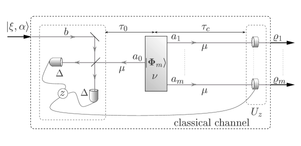
Figure 2: Schematic diagram of the telecloning scheme. After the preparation of the state $|\boldsymbol{\Phi}_{m}\rangle$, a conditional measurement is made on the mode $a_{0}$, which corresponds to the joint measurement of the sum- and difference-quadratures on two modes: mode $a_{0}$ itself and another reference mode $b$, which is excited in a pure Gaussian state $|\xi,\alpha\rangle$, to be teleported and cloned. The result $z$ of the measurement is classically sent to the parties who want to prepare approximate clones, where suitable displacement operations (see text) on modes $a_{1},\dots,a_{m}$ are performed. We indicated with $\nu$ and $\mu$ the mean thermal photons in generation and propagation, whereas $\Delta$ takes into account for the non unit efficiency in the detection stage. The effective propagation times $\tau_{0}$ and $\tau_{c}$ (see Sec. V) are related to the losses during propagation.

After the preparation of the state $|\boldsymbol{\Phi}_{m}\rangle$, a joint measurement is made on modes $a_{0}$ and $b$, which corresponds to measure the complex photocurrent $Z=b+a_{0}^{\dagger}$ (double-homodyne detection), as in the teleportation protocol. The measurement is described by the POVM $\{\Pi(z)\}_{z\in{\mathbb{C}}}$, acting on the mode $a_{0}$, whose elements are given by

$$\Pi(z) =\pi^{-1}D_{a_{0}}(z)\>\varrho_{\rm in}^{\scriptscriptstyle T}D_{a_{0}}^{\dagger}(z)$$

$$=\pi^{-1}S_{a_{0}}(\xi^{*})D_{a_{0}}(z^{\prime})D_{a_{0}}(\alpha^{*})\,|0\rangle\langle 0|\,D^{\dagger}_{a_{0}}(\alpha^{*})D_{a_{0}}^{\dagger}(z^{\prime})S^{\dagger}_{a_{0}}(\xi^{*})\;,$$ (32)

where $z$ is the measurement outcome, $z^{\prime}=z\cosh r+e^{-i\theta}z^{*}\sinh r$, $\xi=re^{i\theta}$ and ^T denotes transposition. The probability distribution of the outcomes is given by

$$P(z) =\hbox{Tr}_{0\dots m}\left[|\boldsymbol{\Phi}_{m}\rangle\langle\boldsymbol{\Phi}_{m}|\>\Pi(z)\bigotimes_{h=1}^{m}\mathbb{I}_{h}\right]$$

$$=\frac{1}{\pi(1+N_{0})}\>\exp\left\{-\frac{|z^{\prime}+\alpha^{*}|^{2}}{1+N_{0}}\right\}\;,$$ (33)

being $\mathbb{I}_{h}$ the identity operator acting on mode $a_{h}$. The conditional state of the remaining modes then reads

$$\varrho_{z} =\frac{1}{P(z)}\>\hbox{Tr}_{0}\left[|\boldsymbol{\Phi}_{m}\rangle\langle\boldsymbol{\Phi}_{m}|\>\Pi(z)\bigotimes_{h=1}^{m}\mathbb{I}_{h}\right]$$

$$=\bigotimes_{h=1}^{m}S_{a_{h}}(\xi)|{\cal C}_{h}(z^{\prime*}+\alpha)\rangle\langle{\cal C}_{h}(z^{\prime*}+\alpha)|S^{\dagger}_{a_{h}}(\xi)\;,$$ (34)

where $|{\cal C}_{h}(z^{\prime*}+\alpha)\rangle$ denotes a coherent state (of the usual Heisenberg Weyl group) with amplitude ${\cal C}_{h}(z^{\prime*}+\alpha)$. After the measurement, the conditional state should be transformed by a further unitary operation, depending on the outcome of the measurement. In our case, this is a $m$-mode product displacement $U_{z}=\bigotimes_{h=1}^{m}D_{h}^{\scriptscriptstyle T}(z)$. This is a local transformation, which generalizes to $m$ modes the procedure already used in the original CV teleportation protocol. The overall state is obtained by averaging over the possible outcomes

$$\varrho_{1\dots m}=\int_{\mathbb{C}}d^{2}z\>P(z)\>\tau_{z}\>.$$

where $\tau_{z}=U_{z}\>\varrho_{z}\>U_{z}^{\dagger}$. Thus, the partial traces $\varrho_{h}=\hbox{Tr}_{1,\dots,h-1,h+1,\dots,m}[\varrho_{1\dots m}]$ read as follows

$$\varrho_{h}=S_{h}(\xi)\,\left[\int_{\mathbb{C}}d^{2}z\>P(z)\>|\alpha\,{\cal C}_{h}+z^{\prime*}\,({\cal C}_{h}-1)\rangle\langle\alpha\,{\cal C}_{h}+z^{\prime*}\,({\cal C}_{h}-1)|\,\right]S^{\dagger}_{h}(\xi)\;.$$ (35)

Upon a changing in the integration variable we obtain the following expression for the clones:

$$\varrho_{h}=S_{h}(\xi)\,\left[\int_{\mathbb{C}}d^{2}w\>\frac{1}{\pi\,n_{h}}\exp\left\{-\frac{|w-\alpha|^{2}}{n_{h}}\right\}\>|w\rangle\langle w|\,\right]S^{\dagger}_{h}(\xi)\;,$$ (36)

where we defined

$$n_{h}=\left(\sqrt{N_{0}+1}-\sqrt{N_{h}}\right)^{2}\,.$$ (37)

From expression (36) one immediately recognize that the clones are given by thermal states $\varrho_{\rm th}(n_{h})$, with mean photon number $n_{h}$, displaced and squeezed by the amounts $\alpha$ and $\xi$ respectively, i.e.:

$$\varrho_{h}=S_{h}(\xi)\,D_{h}(\alpha)\,\varrho_{\rm th}(n_{h})\,D^{\dagger}_{h}(\alpha)\,S^{\dagger}_{h}(\xi)\;.$$ (38)

As a consequence, we see that the protocol acts like a proper covariant Gaussian cloning machine cerf23 , and that the noise introduced by the cloning process is entirely quantified by the thermal photons $n_{h}$, which in turn depend only on the value of the mean photon numbers $N_{h}$ of the shared state. The fidelity $F_{h}$ between the $h$-th clone and the initial state $|\xi,\alpha\rangle$ does not depend on the latter and is given by

$$F_{h}=\frac{1}{1+n_{h}}\,.$$ (39)

The expression of the clones in Eq. (38) says that they can either be equal or different one to each other, depending on the values of the $n_{h}$’s. In other words, a remarkable feature of this scheme is that it is suitable to realize both symmetric, when $n_{2}=\dots=n_{m}=n$, and asymmetric cloning, $n_{2}\neq\dots\neq n_{m}$. This arises as a consequence of the possible asymmetry of the state that supports the telecloning. To our knowledge, this is the first example of a completely asymmetric $1\rightarrow m$ cloning machine for continuous variable systems.

Concerning the symmetric cloning one has that this scheme saturates the bound given in Ref. cerf , hence ensuring the optimality of the protocol. In fact, the minimum added noise for a symmetric $1\rightarrow m$ cloner of coherent states is given by $n=\frac{m-1}{m}$, which in our case can be attained by setting $N_{1}=\dots=N_{m}=N^{\rm opt}$, where

$$N^{\rm opt}=\frac{1}{m(m-1)}$$ (40)

It follows that the fidelity is optimal, namely $F=m/(2m-1)$. It is not surprising that this result is the same as the one obtained in Ref. vLB_tlc . In fact, as already mentioned, the latter uses as support a specific ${\rm SU}(m,1)$ coherent state, generated with a particular interaction built from single mode squeezers and beam-splitters. Our calculation extends this result to any ${\rm SU}(m,1)$ coherent state used to support the telecloning protocol.

IV.1 Asymmetric cloning

Consider now the case of asymmetric cloning. In this case one deals with a true quantum information distributor, in which the information encoded in an original state may be distributed asymmetrically between many parties according to the particular task one desires to attain. In this scenario, a particularly relevant question concerns the maximum fidelity achievable by one party, say $F_{1}$, once the fidelities $F_{j}$ ($j=2,\dots,m$) of the other ones are fixed. Thanks to Eq. (39) we see that this is equivalent to the issue of finding the minimum noise $n_{1}$ introduced by the cloning process for fixed $n_{j}$’s ($n_{j}\neq 1$). The optimization has to be performed under the constrain given by Eq. (2), which allows to write $n_{1}$ as a function of the $n_{j}$’s and of the total mean photon number $N_{0}$ (the sums run for $j=2,\dots,m$):

$$n_{1}=\left[\sqrt{N_{0}+1}-\sqrt{N_{0}-\sum_{j}\left(\sqrt{N_{0}+1}-\sqrt{n_{j}}\right)^{2}}\right]^{2}\;.$$ (41)

The minimum noise $n_{1}^{\rm min}$ is then found setting $N_{0}$ such that

$$(N_{0}+1)(m-1)(m-2)-2\,\sqrt{N_{0}+1}(m-1){\scriptstyle\sum_{j}}\sqrt{n_{j}}+{\scriptstyle\sum_{j}}n_{j}+\left({\scriptstyle\sum_{j}}\sqrt{n_{j}}\right)^{2}-1=0\,.$$ (42)

For $m=2$ one obtains that the optimal choice for $N_{0}$ is given by $N_{0}^{\rm opt}=n_{2}+1/4n_{2}$. It follows that the minimum noise $n_{1}^{\rm min}$ allowed by our telecloning protocol for fixed $n_{2}$ is given by $n_{1}^{\rm min}=1/4n_{2}$. Hence we recover the result of Ref. josab for the fidelities:

$$F_{1}^{\rm max}=\frac{4(1-F_{2})}{4-3F_{2}}\;.$$ (43)

Notice that if one requires $F_{2}=1$ then $F_{1}=0$, that is no information is left to prepare a non-trivial clone on mode $a_{1}$. We remark that the result in Eq. (43) shows that the protocol introduced above, besides reaching the optimal bound in the symmetric case, is optimal also in the case of asymmetric $1\rightarrow 2$ cloning fiurasek . Coming back to the general case we see from Eqs.(41) and (42) that for $m\geq 3$ the minimum noise $n_{1}$ is given by

$$n_{1}^{\rm min}=\frac{1}{(m-2)^{2}}\left\{{\scriptstyle\sum_{j}}\sqrt{n_{j}}-\sqrt{(m-1)\left[({\scriptstyle\sum_{j}}\sqrt{n_{j}})^{2}-(m-2){\scriptstyle\sum_{j}}n_{j}-(m-2)\right]}\right\}^{2}\;,$$ (44)

and it is attained for the following optimal choice of $N_{0}$

$$N_{0}^{\rm opt}=\frac{1}{(m-1)^{2}(m-2)^{2}}\left\{(m-1){\scriptstyle\sum_{j}}\sqrt{n_{j}}-\sqrt{(m-1)\left[({\scriptstyle\sum_{j}}\sqrt{n_{j}})^{2}-(m-2){\scriptstyle\sum_{j}}n_{j}-(m-2)\right]}\right\}^{2}-1\;.$$ (45)

Substituting Eq. (44) in Eq. (39) one then obtains the maximum fidelity $F_{1}^{\rm max}$ achievable for $F_{j}$ fixed. Summarizing, if one fixes the fidelities $F_{j}$ (for $j=2,\dots,m$) then the thermal photons $n_{j}$ are given by Eq. (39), which in turn individuate the mean photon numbers $N_{j}$ and $N_{1}$ of the state that supports the telecloning via Eqs. (37), (44) and (45). This choice guarantees that the fidelity $F_{1}$ is the maximum achievable with the telecloning protocol described above, thus providing the optimal trade-off between the qualities of the different clones.

As an example, consider the fully asymmetric $1\rightarrow 3$ telecloning and fix the couple of fidelities $F_{2}$ and $F_{3}$. Specializing the formulae above we have that, choosing the state $|\boldsymbol{\Phi}_{3}\rangle$ such that:

$$N_{1}=\sqrt{\left(\frac{1}{F_{2}}-1\right)\left(\frac{1}{F_{3}}-1\right)}-\frac{1}{2}\,,\qquad N_{2\,(3)}=\left[\sqrt{\frac{1}{F_{3\,(2)}}-1}-\sqrt{N_{1}}\right]^{2}\,,$$ (46)

then the fidelity of the first clone is the maximal allowed by our scheme, in formulae:

$$F_{1}^{\rm max}=\left\{1+\left[\sqrt{\frac{1}{F_{2}}-1}+\sqrt{\frac{1}{F_{3}}-1}-\sqrt{2\left(2\sqrt{\left(\frac{1}{F_{2}}-1\right)\left(\frac{1}{F_{3}}-1\right)}-1\right)}\right]^{2}\right\}^{-1}\;.$$ (47)

Notice that $F_{1}^{\rm max}$ in Eq. (47) is valid iff the fixed fidelities $F_{2}$ and $F_{3}$ satisfy the relation $F_{2}\leq 4(1-F_{3})/(4-3F_{3})$, which coincides with the optimal relation given by Eq. (43). In other words, the optimal bound imposed by quantum mechanics to $1\rightarrow 2$ telecloning is automatically incorporated into the bound (47) for $1\rightarrow 3$ telecloning of our scheme. When $F_{2}=F_{3}=3/5$ (that is, the bound for an optimal symmetric $1\rightarrow 3$ cloner) we have that $F_{1}^{\rm\max}=3/5$, as one may expect from the discussion above concerning the symmetric cloning case. Remarkably, when $F_{2}=F_{3}=2/3$ (that is, the bound for an optimal symmetric $1\rightarrow 2$ cloner) one has that $F_{1}^{\rm\max}=1/3>0$. This means that, even if two optimal clones have been produced, there still remains some quantum information to produce a non-trivial third clone. A similar situation occurs for the case of cloning with discrete variables, as pointed out in Ref. IblisdirAsym .

Similar results occur for the generic $m$ case. In fact, it can be immediately shown by inspection that substituting $n_{j}=(m-1)/m$ (that is, the bound for the noise introduced by an optimal symmetric $1\rightarrow m$ cloner) in Eq. (44) one obtains $n_{1}^{\rm min}=(m-1)/m$. Hence optimal symmetric cloning is recovered. Similarly, substituting $n_{j}=(m-2)/(m-1)$ (that is, the bound for the noise introduced by an optimal symmetric $1\rightarrow(m-1)$ cloner) in Eq. (44) one obtains $n_{1}^{\rm min}=(m-1)/(m-2)$, from which a fidelity $F_{1}^{\rm max}=\frac{m-2}{2m-3}>0$ follows. This confirms that the production of $(m-1)$ optimal clones still leave some quantum information at disposal to produce an additional non-trivial clone. An explanation for this effect may be individuated recalling that for large $m$ the optimal cloner coincides with an optimal measurement on the original state followed by $m$ reconstruction cerf . As a consequence, one may expect that the production (reconstruction) of $(m-1)$ optimal clones leaves information (i.e., the measurement result) for the reconstruction of other ones.

A question strictly related to the one faced above, and probably more significant from an information distribution viewpoint, is the following. Suppose that one wants to distribute the information encoded in the original state by fixing the ratio between the noise that affects all the $m$ clones, and not by fixing the fidelities of $(m-1)$ clones. More specifically, suppose that one wants to give the minimum noise to, say, the first clone ($n_{j}>n_{1}$ for every $j=2,\dots,m$). Now fix the noise that affects the other clones by fixing their ratio $q_{j}$ with respect to the first one, that is $n_{j}=q_{j}\,n_{1}$. Then, which is the minimum noise $n_{1}^{\rm min}$ allowed by our protocol for fixed $q_{j}$? Solving Eq. (44) for $n_{1}$, one may find the following closed expression for $n_{1}^{\rm min}$ as a function of $q_{j}$:

$$n_{1}^{\rm min}=\frac{m-1}{\left(1+\sum_{j}\sqrt{q_{j}}\right)^{2}-(m-1)\left(1+\sum_{j}q_{j}\right)}\;.$$ (48)

The state $|\boldsymbol{\Psi}_{m}\rangle$ that provides this optimal result is simply given by setting the $N_{1}$ and $N_{j}$’s obtained by substituting back $n_{j}^{\rm min}=q_{j}\,n_{1}^{\rm min}$ in Eq. (45) and Eq. (37).

As a final remark we point out that a general bound for the fidelities in a fully asymmetric $1\rightarrow m$ cloning of coherent states has not yet been derived when $m\geq 3$. As a consequence, we cannot judge if the telecloning process introduced above is in general optimal or not for $m\geq 3$. Nevertheless, there are valuable indications for its optimality, i.e. the fact that it is optimal in the case of $m=2$, and, as we have already pointed out, it is optimal for any $m$ in the symmetric case. In addition, as already mentioned, our telecloning protocol allows to built a non-trivial additional clone when $(m-1)$ optimal ones have been produced.

V Telecloning in a noisy environment

The protocol described in the previous section is referred to the case of ideal generation and propagation of the states $|\boldsymbol{\Psi}_{m}\rangle$ as well as to double-homodyne detection with unit quantum efficiency. In order to take into account the possible losses and noise in the various steps, it is useful to reformulate the whole protocol in the phase space. Consider the characteristic function associated to the states $|\boldsymbol{\Psi}_{m}\rangle$: $\chi[\boldsymbol{\sigma}_{m}](\boldsymbol{\Lambda})=\exp\{-\frac{1}{2}\boldsymbol{\Lambda}^{T}\boldsymbol{\sigma}_{m}\boldsymbol{\Lambda}\}$. The covariance matrix $\boldsymbol{\sigma}_{m}$ given in Eq. (14) can be written accordingly to the following bipartite structure

$$\boldsymbol{\sigma}_{m}=\begin{pmatrix}{\boldsymbol{A}}&{\boldsymbol{C}}\\ {\boldsymbol{C}}^{T}&{\boldsymbol{B}}\end{pmatrix}\,,$$ (49)

where ${\boldsymbol{A}}$ is a $2\times 2$ matrix corresponding to mode $a_{0}$, while ${\boldsymbol{B}}$ and ${\boldsymbol{C}}$ are $2m\times 2m$ and $2\times 2m$ matrices respectively. Consider now a generic Gaussian POVM, acting on modes $a_{0}$ and $b$, defined by a covariance matrix ${\boldsymbol{M}}$ and a vector of first moments ${\boldsymbol{X}}$, i.e., $\chi[{\boldsymbol{M}},{\boldsymbol{X}}](\boldsymbol{\Lambda})=\exp\{-\frac{1}{2}\boldsymbol{\Lambda}^{T}{\boldsymbol{M}}\boldsymbol{\Lambda}-i\boldsymbol{\Lambda}^{T}{\boldsymbol{X}}\}$. The case of the ideal double-homodyne measurement introduced above, corresponds to

$${\boldsymbol{M}}=\mathbb{P}\boldsymbol{\sigma}_{\rm in}\mathbb{P}\,,\qquad{\boldsymbol{X}}=\mathbb{P}\overline{\boldsymbol{X}}+{\boldsymbol{Z}}\,,$$ (50)

where $\boldsymbol{\sigma}_{\rm in}$ and $\overline{\boldsymbol{X}}$ are the covariance matrix and the vector of first moments of the input state (mode $b$), whereas ${\boldsymbol{Z}}=\{\Re\hbox{e}[z],\Im\hbox{m}[z]\}$ is the measurement result [we recall that $\mathbb{P}={\rm Diag}(1,-1)$]. Then, the state conditioned to the result ${\boldsymbol{Y}}$ is given by a Gaussian state with covariance matrix

$$\boldsymbol{\sigma}_{c}={\boldsymbol{B}}-{\boldsymbol{C}}^{T}({\boldsymbol{A}}+{\boldsymbol{M}})^{-1}{\boldsymbol{C}}$$ (51)

and vector of displacements ${\boldsymbol{H}}={\boldsymbol{C}}^{T}({\boldsymbol{A}}+{\boldsymbol{M}})^{-1}{\boldsymbol{X}}$. The protocol is now completed with the proper generalized local displacement introduced in the previous section, i.e., $U_{z}=\bigotimes_{h=1}^{m}D_{h}^{\scriptscriptstyle T}(z)$. Averaging over all the possible outcomes we finally obtain the following expression for the covariance matrix of the Gaussian state at the output besancon :

$$\boldsymbol{\sigma}={\boldsymbol{B}}+\mathbb{J}^{T}\mathbb{P}({\boldsymbol{A}}+{\boldsymbol{M}})\mathbb{P}\mathbb{J}-\mathbb{J}^{T}\mathbb{P}{\boldsymbol{C}}-{\boldsymbol{C}}^{T}\mathbb{P}\mathbb{J}\;,$$ (52)

where $\mathbb{J}$ is given by the $2\times 2m$ matrix $\mathbb{J}=(\openone,\dots,\openone)$.

As already pointed out in Sec. III, if we consider a realistic scenario for the application of the telecloning protocol, we must take into account that the generation and the propagation of the states $|\boldsymbol{\Psi}_{m}\rangle$ are affected by thermal background and losses. In particular, concerning propagation we can consider that modes $a_{1},\dots,a_{m}$ propagate in noisy channels characterized by the same losses $\Gamma_{c}$. We may then define an effective propagation time $\tau_{c}=\Gamma_{c}t$ equal for all the clones, while the effective propagation time $\tau_{0}=\Gamma_{0}t$ for mode $a_{0}$ is left different from $\tau_{c}$. Consider in fact a scenario in which one has two distant location (see Fig. 2): the sending station, where the double-homodyne measurement is performed, and the receiving station, where the clones are eventually retrieved. The distance between the two stations can be viewed as a total effective propagation time $\tau_{\mbox{\tiny$T$}}$ which can be written as $\tau_{{\mbox{\tiny$T$}}}=\tau_{0}+\tau_{c}$. Then, the choice made above corresponds to the possibility of choosing at will, for a given $\tau_{\mbox{\tiny$T$}}$, which modes ($a_{1},\dots,a_{m}$ or $a_{0}$) will be affected by the unavoidable noise that separates the sending and the receiving station and to which extent. With a slight abuse of language, we may say that one can choose whether to put the source of the entangled state $|\boldsymbol{\Psi}_{m}\rangle$ near the sending station ($\tau_{{\mbox{\tiny$T$}}}=\tau_{c}$), near the receiving one ($\tau_{{\mbox{\tiny$T$}}}=\tau_{0}$), or somewhere in between. A similar strategy has been pursued in welsch to optimize the CV teleportation protocol in a noisy environment. In the following, we will see how to determine both the optimal location and the optimal $|\boldsymbol{\Psi}_{m}\rangle$ for a given amount of noise. For the sake of simplicity, the thermal photons $\mu$ will be taken equal in all the noisy channels. As it is natural to expect, in the generation process all the modes will be also considered to be affected by the same amount of noise, characterized by $\nu$ mean thermal photons. As a consequence, the matrix $\boldsymbol{\sigma}_{m}$ in Eq. (49) should be substituted by (see, e.g., Ref. Napoli ) its noisy counterpart:

$$\boldsymbol{\sigma}_{m,{\rm n}}=\mathbb{G}^{1/2}\boldsymbol{\sigma}_{m,{\rm th}}\mathbb{G}^{1/2}+(1-\mathbb{G})\boldsymbol{\sigma}_{\infty,m}$$ (53)

where we have used Eq. (19), and defined

$$\mathbb{G}=e^{-\tau_{0}}\openone\oplus_{j=1}^{m}\,e^{-\tau_{c}}\openone\qquad\boldsymbol{\sigma}_{\infty,m}=(\mu+\mbox{$\frac{1}{2}$})\openone_{2m}$$ (54)

Performing the calculation explicitly, upon defining $\gamma_{c}=e^{-\tau_{c}}$, $\gamma_{0}=e^{-\tau_{0}}$ , $\kappa=\mu+\mbox{$\frac{1}{2}$}$ and $\zeta=1+2\nu$, we obtain:

$$\boldsymbol{\sigma}_{m,\rm n}=\begin{pmatrix}\widetilde{\boldsymbol{A}}&\widetilde{\boldsymbol{C}}\\ \widetilde{\boldsymbol{C}}\,\!^{T}&\widetilde{\boldsymbol{B}}\end{pmatrix}\,,$$ (55)

where $\widetilde{\boldsymbol{A}}=\zeta\,[\gamma_{0}\boldsymbol{\cal N}_{0}+\frac{\kappa}{\zeta}(1-\gamma_{0})\openone]$, $\widetilde{\boldsymbol{C}}=\zeta\,\sqrt{\gamma_{0}\,\gamma_{c}}\,{\boldsymbol{C}}$ and

$$\widetilde{\boldsymbol{B}}=\zeta\left(\begin{array}[]{ccccc}\gamma_{c}\boldsymbol{\cal N}_{1}+\frac{\kappa}{\zeta}(1-\gamma_{c})\openone&\gamma_{c}\boldsymbol{\cal B}_{1,2}&\ldots&\gamma_{c}\boldsymbol{\cal B}_{1,m}\\ \gamma_{c}\boldsymbol{\cal B}_{1,2}&\gamma_{c}\boldsymbol{\cal N}_{2}+\frac{\kappa}{\zeta}(1-\gamma_{c})\openone&\ddots&\vdots\\ \vdots&\ddots&\ddots&\gamma_{c}\boldsymbol{\cal B}_{m-1,m}\\ \gamma_{c}\boldsymbol{\cal B}_{1,m}&\ldots&\gamma_{c}\boldsymbol{\cal B}_{m-1,m}&\gamma_{c}\boldsymbol{\cal N}_{m}+\frac{\kappa}{\zeta}(1-\gamma_{c})\openone\\ \end{array}\right)\,.$$ (60)

A non-unit efficiency $\eta$ in the detection stage corresponds to have the covariance matrix of the double-homodyne detection given by $\widetilde{\boldsymbol{M}}=\mathbb{P}\boldsymbol{\sigma}_{\rm in}\mathbb{P}+\frac{1}{2}\Delta\openone$ (where $\Delta=\frac{1-\eta}{\eta}$). Finally, considering an initial coherent state note2 and recalling Eq. (52), we have $\widetilde{\boldsymbol{M}}=\frac{1}{2}(1+\Delta)\openone$, whereas the covariance matrix of the $m$ output modes now reads:

$$\boldsymbol{\sigma}_{\rm n}=\widetilde{\boldsymbol{B}}+\mathbb{J}^{T}\mathbb{P}(\widetilde{\boldsymbol{A}}+\widetilde{\boldsymbol{M}})\mathbb{P}\mathbb{J}-\mathbb{J}^{T}\mathbb{P}\widetilde{\boldsymbol{C}}-\widetilde{\boldsymbol{C}}\,\!^{T}\mathbb{P}\mathbb{J}\;,$$ (61)

which in turn gives the following covariance matrix for the $h$-th clone:

$$\boldsymbol{\sigma}_{h,{\rm n}}=\left(\frac{1}{F_{h}}-\frac{1}{2}\right)\openone\,.$$ (62)

In the Equation above, $F_{h}$ represents the fidelity between the $h$-th clone and the original coherent state:

$$F_{h} =\left\{{\rm Det}\,\left[\boldsymbol{\sigma}_{h,{\rm n}}+\mbox{$\frac{1}{2}$}\openone\right]\right\}^{-1/2}$$

$$=\left\{1+\frac{\Delta}{2}+2\kappa+\zeta\left[\gamma_{0}\left(N_{0}+\frac{1}{2}-\frac{\kappa}{\zeta}\right)+\gamma_{c}\left(N_{h}+\frac{1}{2}-\frac{\kappa}{\zeta}\right)-2\,\sqrt{\gamma_{0}\,\gamma_{c}\,N_{h}(N_{0}+1)}\right]\right\}^{-1}\,.$$ (63)

V.1 Optimization of the symmetric protocol

In order to clarify the implication of the formula (V), let us focus our attention to the case of symmetric cloning (recall that in this case $N_{1}=\ldots=N_{m}=N$). Upon defining $x=\frac{\kappa}{\zeta}-\frac{1}{2}$, $\gamma_{\mbox{\tiny$T$}}=e^{-\tau_{\mbox{\tiny$T$}}}=\gamma_{0}\gamma_{c}$ and the following function

$$f(N,\gamma_{0};x,\gamma_{\mbox{\tiny$T$}})=\frac{\gamma_{\mbox{\tiny$T$}}}{\gamma_{0}}(N-x)+\gamma_{0}(m\,N-x)-2\,\sqrt{\gamma_{\mbox{\tiny$T$}}N(m\,N+1)}\;,$$ (64)

the fidelity reads as follows

$$F=\left\{\zeta\,f(N,\gamma_{0};x,\gamma_{\mbox{\tiny$T$}})+2\,\kappa+1+\frac{\Delta}{2}\right\}^{-1}\,.$$ (65)

Our aim is now to optimize, for a fixed amount of noise, the shared state $|\boldsymbol{\Psi}_{m}\rangle$ and the location of its source between the sending and the receiving station. Namely, one has to find $N$ and $\gamma_{0}$ which maximize the fidelity $F$ for $\gamma_{\mbox{\tiny$T$}}$, $\kappa$, $\zeta$, $\Delta$ fixed. This, in turn, means to minimize $f(N,\gamma_{0};x,\gamma_{\mbox{\tiny$T$}})$ for fixed $\gamma_{\mbox{\tiny$T$}}$ and $x$. The domain where to perform the minimization is the region $N>0$ and $\gamma_{T}<\gamma_{0}<1$. We will see that the possibility of varying $\gamma_{0}$ will reveal crucial in order to adapt the ideal cloning protocol, presented in Sec. IV, to a noisy environment.

Calculating the stationary points of $f(N,\gamma_{0};x,\gamma_{\mbox{\tiny$T$}})$ one finds:

$$s_{1} =\left\{N=\frac{x}{1-x(m-1)}\,,\,\gamma_{0}=\sqrt{\frac{\gamma_{\mbox{\tiny$T$}}\,x}{x+1}}\right\}\,,$$

$$s_{2} =\left\{N=\frac{x}{m[1+x(m-1)]}\,,\,\gamma_{0}=\sqrt{\frac{\gamma_{\mbox{\tiny$T$}}\,(1+m\,x)}{m\,x}}\right\}\,.$$ (66)

The points $s_{1}$ and $s_{2}$ belong to the domain for $\left\{\gamma_{\mbox{\tiny$T$}}<\frac{x}{x+1}\,,x<\frac{1}{m-1}\right\}$ and for $\left\{\gamma_{\mbox{\tiny$T$}}<\frac{m\,x}{m\,x+1}\,,\forall x\right\}$ respectively. By evaluating the Hessian matrix associated to $f(N,\gamma_{0};x,\gamma_{\mbox{\tiny$T$}})$, it follows that both $s_{1}$ and $s_{2}$ are not extremal points. As a consequence one has to look for the minimum of $f(N,\gamma_{0};x,\gamma_{\mbox{\tiny$T$}})$ along the boundary of the minimization domain. Three local minima are found in the three regions parametrized by $\gamma_{0}=\gamma_{\mbox{\tiny$T$}}$, $\gamma_{0}=1$ and $N\rightarrow\infty$, whereas the forth extremum is a maximum. In particular, in the first region the minimum is attained for

$$N=\left\{\begin{array}[]{ll}-\dfrac{\gamma_{\mbox{\tiny$T$}}}{m\gamma_{\mbox{\tiny$T$}}-1}&\;\gamma_{T}>1/m\\ \dfrac{1}{m(m\gamma_{\mbox{\tiny$T$}}-1)}&\;\gamma_{T}<1/m\end{array}\right.$$ (69)

Concerning the second and the third region, one finds that the minima are located at

$$N=-\frac{\gamma_{\mbox{\tiny$T$}}}{m(\gamma_{\mbox{\tiny$T$}}-m)}$$ (70)

and at

$$\gamma_{0}=\sqrt{\frac{\gamma_{\mbox{\tiny$T$}}}{m}}\;,$$ (71)

respectively. By evaluating the value of $f(N,\gamma_{0};x,\gamma_{\mbox{\tiny$T$}})$ in the minima, one eventually attain the global maximum $F^{\rm max}$ of the fidelity. A summary of the results is given in Tab. 1, where we have reintroduced the effective propagation times $\tau_{{\mbox{\tiny$T$}}}$, $\tau_{0}$ and defined the following quantities:

$$F^{a} =\frac{2\,m}{-2-4\,\nu+m\left\{\Delta+2\left[2+\mu+\nu+(\nu-\mu)e^{-\tau_{\mbox{\tiny$T$}}}\right]\right\}}\,,$$ (72)

$$F^{b} =2\left\{\Delta+2(2+\mu+\nu)-2\,(1+\mu+\nu)e^{-\tau_{\mbox{\tiny$T$}}}\right\}^{-1}\,,$$ (73)

$$F^{c} =\bigg{\{}2+\frac{\Delta}{2}+2\mu-\sqrt{\frac{e^{-\tau_{\mbox{\tiny$T$}}}}{m}}\left[1+\mu+\nu+m(\mu-\nu)\right]\bigg{\}}^{-1}\,.$$ (74)

$x$	$\tau_{\mbox{\tiny$T$}}$	$\tau_{0}^{\rm opt}$	$N^{\rm opt}$	$F^{\rm max}$
$\forall x$	$0<\tau_{\mbox{\tiny$T$}}<\ln m$	$\tau_{\mbox{\tiny$T$}}$	${\displaystyle\frac{1}{m(m\,e^{-\tau_{\mbox{\tiny$T$}}}-1)}}$	$F^{a}$
$-\frac{1}{2}<x<0$	$\tau_{\mbox{\tiny$T$}}>\ln m$	$\mbox{$\frac{1}{2}$}(\tau_{\mbox{\tiny$T$}}+\ln m)$	$N\rightarrow\infty$	$F^{c}$
$0<x<\frac{1}{m-1}$	${\displaystyle\ln m<\tau_{\mbox{\tiny$T$}}<\ln\left[\frac{(1+x)^{2}}{m\,x^{2}}\right]}$	$\mbox{$\frac{1}{2}$}(\tau_{\mbox{\tiny$T$}}+\ln m)$	$N\rightarrow\infty$	$F^{c}$
	$\tau_{\mbox{\tiny$T$}}>\ln\frac{(1+x)^{2}}{m\,x^{2}}$	$\tau_{\mbox{\tiny$T$}}$	${\displaystyle\frac{e^{-\tau_{\mbox{\tiny$T$}}}}{1-m\,e^{-\tau_{\mbox{\tiny$T$}}}}}$	$F^{b}$
$x>\frac{1}{m-1}$	$\tau_{\mbox{\tiny$T$}}>\ln m$	$\tau_{\mbox{\tiny$T$}}$	${\displaystyle\frac{e^{-\tau_{\mbox{\tiny$T$}}}}{1-m\,e^{-\tau_{\mbox{\tiny$T$}}}}}$	$F^{b}$

Table 1: Values of the optimized $N^{\rm opt}$ and $\tau_{0}^{\rm opt}$ for fixed values of $\tau_{\mbox{\tiny$T$}}$ and $x$. The value reached by the fidelity $F^{\rm max}$ for these optimal choices is given in the last column.

An inspection of Tab. 1 shows very interesting features of the telecloning protocol in presence of noise. It is immediate to recognize that the optimal value $N^{\rm opt}$ is significantly different from the optimal value in the ideal case [Eq. (40)]. As a matter of fact $N^{\rm opt}$ is divergent in some cases. Remarkably, in the optimization of $N$ and $\tau_{0}$ the homodyne detection efficiency $\Delta$ plays no role, whereas the thermal noises $\mu$ and $\nu$ introduce a dependence on $x$, i.e. only on their ratio. Furthermore, one may note that what we have called the best location of the source (that is $\tau_{0}^{\rm opt}$) is never given by the simple choices $\tau_{0}=0$ or $\tau_{0}=\tau_{\mbox{\tiny$T$}}/2$. In order to clarify this point let us first consider the case $\tau_{0}=0$, which can be physically implemented by homodyning mode $a_{0}$ immediately after the generation of $|\boldsymbol{\Psi}_{m}\rangle$, and then letting the other modes propagate to the receiving station where they are eventually displaced. An immediate calculation shows that in this case the fidelity (65) is maximized for $N^{\rm opt}=1/m(m\,e^{\tau_{\mbox{\tiny$T$}}}-1)$ and is given by

$$F^{\rm max}(\tau_{0}=0)=\frac{2\,m}{2\,e^{\tau_{\mbox{\tiny$T$}}}\left[1+m(\mu-\nu)+2\,\nu\right]-m\left[\Delta+2(2+\mu+\nu)\right]}\;.$$ (75)

Concerning the case $\tau_{0}=\tau_{\mbox{\tiny$T$}}/2$, whose physical implementation simply means to put the source of $|\boldsymbol{\Psi}_{m}\rangle$ in the middle of the transmission line, one has that the fidelity is maximized for $N^{\rm opt}=1/m(m-1)$ and reads

$$F^{\rm max}(\tau_{0}=\tau_{\mbox{\tiny$T$}}/2)=\frac{2\,m}{m(4+\Delta+4\,\mu)-2e^{-\tau_{\mbox{\tiny$T$}}/2}\left[1+2\,\nu+2\,m(\mu-\nu)\right]}\;.$$ (76)

Notice that only in this case the optimization over $N$ leads to the same $|\boldsymbol{\Psi}_{m}\rangle$ as in the ideal case (see Eq. (40)). A comparison of the last two instances with the optimal one, shows how significantly the choice of $\tau_{0}$ affects the value of the clones’ fidelity. In Figs. 3, 4 and 5 we compared the two fidelities given in Eqs. (75) and (76) with the one given in Tab. 1 (see captions for details). We clearly see that the optimized fidelity is much larger then the other two, thus providing a cloning beyond the classical limit for higher propagation times $\tau_{\mbox{\tiny$T$}}$. As it is apparent from Fig. 5 we have $F^{b}<\frac{1}{2}$ $\forall\tau_{\mbox{\tiny$T$}}$. Indeed, it can be shown analitically that $F^{b}<\frac{1}{2}$ in any regime for which $F^{\rm max}=F^{b}$.

Figure 3: Comparison of the fidelities given in Eqs. (75) (dotted line) and (76) (dashed line) with the one given in Tab. 1 (solid line). As an example, we have chosen the following parameters: $\mu=0.03$, $\nu=0.01$ and $\Delta=0.02$ ($x=1/51$). The plots are referred to the case $m=2,5,10$ and the vertical line corresponds to $\tau_{\mbox{\tiny$T$}}=\ln 2$, $\tau_{\mbox{\tiny$T$}}=\ln 5$ and $\tau_{\mbox{\tiny$T$}}=\ln 10$ respectively. Accordingly to Tab. 1, the optimal fidelity is given by Eq. (72) and Eq. (74) at the left and at the right of the vertical lines, respectively.

Figure 4: Comparison of the fidelities given in Eqs. (75) (dotted line) and (76) (dashed line) with the one given in Tab. 1 (solid line). As an example of the case $\mu<\nu$, we have chosen the following parameters: $\mu=0.05$, $\nu=0.2$ and $\Delta=0.05$ ($x=-3/28$). The plots are referred to the case $m=2,3,5$ and the vertical line corresponds to $\tau_{\mbox{\tiny$T$}}=\ln 2$, $\tau_{\mbox{\tiny$T$}}=\ln 3$ and $\tau_{\mbox{\tiny$T$}}=\ln 5$ respectively. Accordingly to Tab. 1, the optimal fidelity is given by Eq. (72) and Eq. (74) at the left and at the right of the vertical lines, respectively.

Figure 5: Comparison of the fidelities given in Eqs. (75) (dotted line) and (76) (dashed line) with the one given in Tab. 1 (solid line). As an example, we have chosen the following parameters: $\mu=0.6$, $\nu=0.01$ and $\Delta=0.1$ ($x=59/102$). The plots are referred to the case $m=2,3$ and the vertical line corresponds to $\tau_{\mbox{\tiny$T$}}=\ln 2$ and $\tau_{\mbox{\tiny$T$}}=\ln 3$ respectively. Accordingly to Tab. 1, for $m=2$ the optimal fidelity is given by Eq. (72) and Eq. (74) at the left and at the right of the vertical line, respectively. For $m=3$, it is instead given by Eq. (73) at the right of the vertical line.

Besides what we pointed out above, the most striking feature of the proposed telecloning protocol is that it saturates the bound for optimal cloning even in the presence of losses, for propagation times $\tau_{\mbox{\tiny$T$}}<\ln m$, hence divergent as the number of modes increases. More specifically, consider the first row in Tab. 1 and set $\mu=\nu=\Delta=0$. Then, one has that for $\tau_{\mbox{\tiny$T$}}<\ln m$ the maximum fidelity is given by $F^{\rm max}=m/(2m-1)$. That is, the optimal fidelity for a symmetric cloning can still be attained, carefully choosing $N$ and $\tau_{0}$. Such a result cannot be achieved letting the input state propagate directly to the receiving station and then cloning it locally besancon . Thus, in the context of our protocol the entangled resource significantly enhances the capacity of distributing quantum information. This is due to the fact that the transmission through a lossy channel of an unknown coherent state irreversibly degrades the information encoded in it, thus avoiding the local construction of optimal clones at the receiving station. On the other hand, multimode entanglement is robust against this type of noise and, even if decreased along the transmission line, it is still sufficient to provide optimal cloning. Actually, there is no need of an infinite amount of entanglement to perform an optimal telecloning process.

As concern the case of higher transmission times, i.e. $\tau_{\mbox{\tiny$T$}}>\ln m$, the fidelity reads (again for $\mu=\nu=\Delta=0$)

$$F^{\rm max}=\left(2-\sqrt{\frac{e^{-\tau_{\mbox{\tiny$T$}}}}{m}}\right)^{-1}.$$ (77)

Eq. (77) shows that the fidelity is always greater then the classical bound $F=\frac{1}{2}$, which in turn means that the state used to support the protocol is entangled for any $\tau_{\mbox{\tiny$T$}}$. This is reminiscent of the result already pointed out in Sec. III, where the full inseparability has been proved for any $\tau_{\mbox{\tiny$T$}}$ for $m=2$ (notice that $\tau_{0}=\tau_{\mbox{\tiny$T$}}/2$ in case of Sec. III). Here, we proved that the same conclusion is valid for any $m$.

Another interesting feature in the case $\tau_{\mbox{\tiny$T$}}<\ln m$ is that $F^{\rm max}$ does not depend on $\tau_{\mbox{\tiny$T$}}$ if $\mu=\nu$. Indeed, it turns out that for $\mu=0$ and $\nu\neq 0$ it is better to let the entangled resource propagate (up to $\tau_{T}=\ln m$) instead of using it immediately after the generation. This effect may be naively understood by considering that the entangled state generated for $\nu\neq 0$ is mixed and, as consequence, the propagation in a purely dissipative environment acts like a sort of purification process on it. As it is apparent from Eq. (72) this effect is present whenever $\mu<\nu$ (see also Fig. 4).

Finally, a comment is needed concerning the scaling of the fidelity with respect to the number of modes $m$. We have already pointed out that for the case $\mu=\nu=\Delta=0$ the fidelity remains optimal for times $\tau_{\mbox{\tiny$T$}}$ diverging with the number of modes. However, when thermal noise is added ($\mu,\nu,\Delta\neq 0$) the fidelity goes below the classical value $F=\frac{1}{2}$ for times $\tau_{\mbox{\tiny$T$}}$ that become smaller as $m$ increases, as it is apparent from Figs. 3, 4 and 5. Indeed, this is consistent with the fact that the optimal fidelity itself approaches the classical value $F=\frac{1}{2}$ as $m$ increases. Hence, even a small amount of thermal noise is enough to cancel the benefits due to quantum entanglement.

VI Conclusions

In this paper we have dealt with the properties and applications of a class of multimode states of radiation, the coherent states of group ${\rm SU}(m,1)$, which represent a potential resource for multiparty quantum communication, as recent theoretical and experimental investigation have shown. In particular, the common structure of these multimode states allowed to consider a $1\rightarrow m$ telecloning scheme in which a generic coherent state of ${\rm SU}(m,1)$ plays the role of entangled resource. Exploiting the possible asymmetry of ${\rm SU}(m,1)$ coherent states we have suggested the first example, in the framework of CV systems, of a fully asymmetric $1\rightarrow m$ cloning and have found the optimal relation, within our scheme, between the different fidelities of the clones. In particular, we have shown that when $(m-1)$ optimal clones are produced (accordingly to the general bound imposed by quantum mechanics), there still remains some quantum information at disposal. In fact, our protocol is able to use the remaining information to realize a non-trivial $m$-th clone. Our asymmetric scheme is aimed at the distribution of quantum information among many parties qid , and may find application for quantum cryptographic purposes gisin .

In view of possible applications of our protocol in realistic situations, we have considered the effects of noise in the various stages of the protocol, i.e. the presence of thermal photons in the generation process, thermal noise and losses during propagation, and non-unit efficiency in the detection. We have derived the fidelities of the clones as a function of the noise parameters, which in turn allowed for adaptive modification of the protocol to face the detrimental effects of noise. In particular, we have shown that the optimal entangled resource in the presence of noise is significantly different from the one in the ideal case. Also the location of the source plays a prominent role. In fact, we have demonstrated that the optimal location is neither in the middle between the sender and the receiver, nor at the sender station. A striking feature of the optimized protocol is that, even in the presence of losses along the propagation line, the clones’ fidelity remains maximal, a result which is not achievable by means of direct transmission followed by local cloning. This happens for propagation times that diverge as the number of modes increases. We then conclude that our optimized telecloning protocol is robust against noise.

References

- (1) S. L. Braunstein and P. van Loock, Rev. Mod. Phys., in press; e-print, quant-ph/0410100.
- (2) A. Ferraro, S. Olivares and M. G. A. Paris, “Gaussian States in Quantum Information ”, Napoli Series on Physics and Astrophysics (Bibliopolis, Napoli, 2005); e-print, quant-ph/0503237.
- (3) J. Jing et al., Phys. Rev. Lett. 90, 167903 (2003); T. Aoki et al., Phys. Rev. Lett. 91, 080404 (2003); H. Yonezawa, T. Aoki and A. Furusawa, Nature 431, 430 (2004); R. C. Pooser and O. Pfister, e-print, quant-ph/0505130.
- (4) M. E. Smithers and E. Y. C. Lu, Phys. Rev. A 10, 1874 (1974).
- (5) R. R. Puri, Phys. Rev. A 50, 5309 (1994)
- (6) P. van Loock and S. Braunstein, Phys. Rev. Lett. 87, 247901 (2001).
- (7) M. Bondani et al., Opt. Lett. 29, 180 (2004);
- (8) A. V. Rodionov and A. S. Chirkin, Pis’ma Zh. Éksp. Teor. Fiz. 79, 311 (2004) [JETP Lett. 79, 253 (2004)]; J. Guo et al., Phys. Rev. A 71, 034305 (2005).
- (9) N. Piovella, M. Cola and R. Bonifacio, Phys. Rev. A 67, 013817 (2003).
- (10) S. Pirandola et al., Phys. Rev. A 68, 062317 (2003).
- (11) N. Takei et al., e-print quant-ph/0501086.
- (12) M. Murao et al., Phys. Rev. A 59, 156 (1999).
- (13) N. J. Cerf and S. Iblisdir, Phys. Rev. A 62, 040301 (2000).
- (14) S. L. Braunstein et al., Phys. Rev. Lett. 86, 4938 (2001).
- (15) J. Fiurás̆ek, Phys. Rev. Lett. 86, 4942 (2001).
- (16) U. L. Andersen, V. Josse and G. Leuchs, Phys. Rev. Lett. 94, 240503 (2005).
- (17) J. Zhang, C. Xie and K. Peng, e-print quant-ph/0503184.
- (18) A. Ferraro et al., J. Opt. Soc. Am. B 21, 1241 (2004).
- (19) M. Horodecki, P. Horodecki and R. Horodecki, Phys. Lett. A 223, 1 (1996); A. Peres, Phys. Rev. Lett. 77, 1413 (1996).
- (20) L. Duan et al., Phys. Rev. Lett. 84, 2722 (2000).
- (21) R. Simon, Phys. Rev. Lett. 84, 2726 (2000).
- (22) G. Giedke et al., Phys. Rev. A 64, 052303 (2001).
- (23) X. Y. Chen, Phys. Lett. A 335, 121 (2005).
- (24) P. van Loock and S. Braunstein, Phys. Rev. Lett. 84, 3482 (2000).
- (25) A. Serafini et al., J. Opt. B 7, R19 (2005).
- (26) J. Lee, M. S. Kim and H. Jeong, Phys. Rev. A 62, 032305 (2000); S. Olivares, M. G. A. Paris and A. R. Rossi, Phys. Lett. A 319, 32 (2003).
- (27) N. J. Cerf, A. Ipe and X. Rottenberg, Phys. Rev. Lett. 85 1754 (2000).
- (28) Notice that state (31) does not belong to the class of the coherent states of anymore. Nevertheless being the additional squeezing operations local, then all the entanglement used to support the telecloning process is furnished by .
- (29) S. Iblisdir et al., e-print quant-ph/0411179; S. Iblisdir et al., e-print quant-ph/0505152.
- (30) A. Ferraro and M. G. A. Paris, e-print quant-ph/0506168.
- (31) A. V. Chizhov, L. Knöll and D.-G. Welsch, Phys. Rev. A 65, 022310 (2002).
- (32) The protocol can be straightforwardly generalized to squeezed states as in the ideal case.
- (33) S. L. Braunstein, V. Buzek and M. Hillary, Phys. Rev. A 63, 052313 (2001).
- (34) N. Cerf et al., Phys. Rev. Lett. 88, 127902 (2002).