QED of lossy cavities: operator and quantum-state input-output relations

Abstract

Within the framework of exact quantization of the electromagnetic field in dispersing and absorbing media the input-output problem of a high-$Q$ cavity is studied, with special emphasis on the absorption losses in the coupling mirror. As expected, the cavity modes are found to obey quantum Langevin equations, which could be also obtained from quantum noise theories, by appropriately coupling the cavity modes to dissipative systems, including the effect of the mirror-assisted absorption losses. On the contrary, the operator input-output relations obtained in this way would be incomplete in general, as the exact calculation shows. On the basis of the operator input-output relations the problem of extracting the quantum state of an initially excited cavity mode is studied and input-output relations for the $s$-parameterized phase-space function are derived, with special emphasis on the relation between the Wigner functions of the quantum states of the outgoing field and the cavity field.

I Introduction

The use of atoms interacting with light has been very promising in handling information storage, communication, and computation Monroe (2002); Pellizzari et al. (1995); Knill et al. (2001); van Enk et al. (1998); Tregenna et al. (2002). In fact, optical systems do not only allow the observation of fundamental quantum effects Hagley et al. (1997); Doherty et al. (2000); Pinkse et al. (2000); Hood et al. (2000), but they can be also used to implement quantum networks with photons, which may be regarded as representing the best qubit carriers for fast and long-distance quantum communication Pan et al. (2003); Bennett and DiVincenzo (2000). In optical systems resonatorlike devices—referred to as cavities in the following—are indispensable elements. In particular, high-$Q$ cavities have been well known to offer a number of possibilities to engineer nonclassical states of light Raimond et al. (2001); Lange and Kimble (2000).

Since high-$Q$ cavities feature well-pronounced line spectra of the electromagnetic field, which renders it possible to control the atom-field interaction to a high degree, they are best suited for the generation of quantum states on demand. For example, in Ref. Law and Eberly (1995) the creation of arbitrary superposition of Fock states of light inside a cavity by means of controlling the time sequence of the amplitudes and phases of the atom-field interactions of the quantized cavity field and the external driving fields with a trapped atom is considered. Another proposal to generate superposition Fock states or coherent states in a cavity is to exploit adiabatic interaction of the cavity field with an atomic system by achieving the transfer of ground-state Zeeman coherence onto the cavity-mode field Parkins et al. (1995). It is worth noting that the idea of the generation of a bit-stream of single photons on demand in an optical cavity is based on the concept of adiabatic passage Law and Kimble (1997); Hennrich et al. (2000); Kuhn et al. (2002). In the specific context of microwave cavities, a scheme proposed in Domokos et al. (1998) for the generation of photon number states on demand via $\pi$ pulse interaction of single two-level atoms passing through a cavity, has been experimentally realized dBrattke et al. (2001); Walther (2002).

To measure the quantum state of a cavity field, various schemes have been considered. As has been demonstrated experimentally Nogues et al. (2000); Bertet et al. (2002), the quantum state of a microwave cavity field can be reconstructed by employing the dispersive interaction of a single circular Rydberg atom with the cavity field Lutterbach and Davidovich (1997). To reconstruct the quantum state of a cavity field by measuring the field escaping from the cavity, the proposal has been made to use pulsed homodyne detection and an operational definition of the Wigner function in terms of appropriately chosen collective mode operators Santos et al. (2001).

However, to further use intracavity-generated photonic quantum states in applications such as quantum networks connecting distant quantum processors and memories, the issue of extraction from the cavities of the quantum states needs to be considered very carefully with respect to quantum decoherence. In the scheme in Refs. Cirac et al. (1997); van Enk et al. (1999) qubits that are stored in the internal states of cold atoms, located in the antinodes of a standing wave of a high-$Q$ optical cavity are mapped onto photon number states, which play the role of a communication channel by leaking out of the cavity and being caught in a second cavity. Further, schemes for the generation of entangled states of individual atoms held in distant cavities have been considered (see, e.g., Refs. Browne et al. (2003); Clark et al. (2003); Di Fidio and Vogel (2003)). In all the schemes the absorption losses unavoidably occurring in the processes of exit and entrance of the photons through the coupling mirrors are typically disregarded. However, even if from the point of view of classical optics these unwanted losses are very small, so that they effectively do not influence classical light, they can lead to a drastic degradation of nonclassical light features indispensable for quantum communication (see, e.g., Ref. Scheel and Welsch (2001)).

Roughly speaking, there have been two routes of treating the input-output problem of a leaky cavity. In the first—the quantum stochastic approach to the problem—standard Markovian damping theory is employed, where the dynamical system is identified with a chosen mode of the perfect cavity ( $Q$ $\!\to$ $\!\infty$), the dissipative system is identified with the continuum of modes outside the cavity, and a bilinear coupling energy between the modes of the two systems is assumed Collett and Gardiner (1984). In this way, the cavity mode is found to obey a quantum Langevin equation, and operator input-output relations can be derived. The theory can be used, e.g., to relate correlation functions of the outgoing field to correlation functions of the cavity field and the incoming field Gardiner and Collett (1985) or to describe the coupling of modes of two cavities through their respective input and output ports Gardiner (1993); Carmichael (1993).

In the second route—the quantum field theoretical approach to the problem—the calculations are based on Maxwell’s equations and exact quantization of the electromagnetic field in the presence of nonabsorbing cavity walls described in terms of appropriately chosen real permittivities Knöll et al. (1987); Dutra and Nienhuis (2000); Viviescas and Hackenbroich (2003). Having established the equivalence of the two routes, thereby constructing the interaction energy between the cavity field and the outer field, one may try to include unwanted absorption losses in the theory by allowing for further dissipative systems in such a way that appropriately chosen interaction energies between them and the cavity modes are added to the Hamiltonian used in the quantum stochastic approach Viviescas and Hackenbroich (2003); Khanbekyan et al. (2004). As we will show within the frame of exact quantum electrodynamics in dispersing and absorbing media, this simple concept, though leading to the correct quantum Langevin equations for the cavity field, does not lead to the correct operator input-output relations in general, because the absorption losses in the coupling mirrors are not properly taken into account.

If the operator input-output relations are known, the correlation functions of the outgoing field can be expressed in terms of correlation functions of the cavity field and the incoming field. In this context the question of the calculation of outgoing-field quantum state as a whole arises. Starting with the correct operator input-output relations that include both wanted and unwanted losses, we will calculate the quantum state of the pulselike field escaping from a high-$Q$ cavity, assuming that the quantum state of the corresponding cavity field at some initial time is known.

The paper is organized as follows. In Sec. II some basic equations are given and the cavity model is introduced. The intracavity field and the outgoing field, including the operator input-output relations, are studied in Secs. III and IV, respectively. The problem of extraction of an initially prepared cavity-quantum state is considered in Sec. V, and a summary and concluding remarks are given in Sec. VI. Some derivations are given in appendices.

II Preliminaries

II.1 Quantization scheme

Let us consider $N$ atoms (with the $A$th atom being at position $\mathbf{r}_{A}$) that in electric dipole approximation interact with the electromagnetic field in the presence of linear dielectric media of spatially varying and frequency-dependent complex permittivity

$$\varepsilon({\bf r},\omega)=\varepsilon^{\prime}({\bf r},\omega)+i\varepsilon^{\prime\prime}({\bf r},\omega).$$ (1)

Note that due to causality the real and imaginary parts $\varepsilon^{\prime}({\bf r},\omega)$ and $\varepsilon^{\prime\prime}({\bf r},\omega)$, respectively, are uniquely related to each other through the Kramers-Kronig relations. Following the approach to quantization of the macroscopic Maxwell field as given in Refs. Gruner and Welsch (1996); Scheel et al. (1998); Knöll et al. (2001); Scheel et al. (1999); Dung et al. (2000), we may write the multipolar-coupling Hamiltonian in the form of tex

$$\hat{H}=\hat{H}_{\mathrm{field}}+\hat{H}_{\mathrm{atom}}+\hat{H}_{\mathrm{int}}.$$ (2)

Here,

$$\hat{H}_{\mathrm{field}}=\int\!\mbox{\rm d}^{3}{r}\int_{0}^{\infty}\!\mbox{\rm d}\omega\,\hbar\omega\,\hat{\bf{f}}^{\dagger}({\bf r},\omega)\cdot\hat{\bf{f}}({\bf r},\omega)$$ (3)

is the Hamiltonian of the system composed of the electromagnetic field and the medium, including a reservoir necessarily associated with material absorption, with $\hat{\bf{f}}({\bf r},\omega)$ [and $\hat{\bf{f}}^{\dagger}({\bf r},\omega)$] being bosonic fields that play the role of the dynamical variables of the composed system,

$$\bigl{[}\hat{f}_{\mu}({\bf r},\omega),\hat{f}_{\mu^{\prime}}^{\dagger}({\bf r}^{\prime},\omega^{\prime})\bigr{]}=\delta_{\mu\mu^{\prime}}\delta(\omega-\omega^{\prime})\delta^{(3)}({\bf r}-{\bf r}^{\prime}),$$ (4)

$$\bigl{[}\hat{f}_{\mu}({\bf r},\omega),\hat{f}_{\mu^{\prime}}({\bf r}^{\prime},\omega^{\prime})\bigr{]}=0$$ (5)

(the Greek letters label the Cartesian components). Further,

$$\hat{H}_{\mathrm{atom}}=\sum_{A}\sum_{k}\hbar\omega_{Ak}\hat{S}_{Akk}$$ (6)

is the atomic Hamiltonian and

$$\hat{H}_{\mathrm{int}}=-\sum_{A}\hat{\bf{d}}_{A}\cdot\hat{\bf{E}}({\bf r}_{A})$$ (7)

is the (multipolar-)interaction energy, where

$$\hat{S}_{Ak^{\prime}k}=|k^{\prime}\rangle_{A}{{}_{A}}\!\langle k|$$ (8)

are the flip operators of the $A$th atom,

$$\hat{\bf{d}}_{A}=\sum_{kk^{\prime}}{\bf d}_{Akk^{\prime}}\hat{S}_{Akk^{\prime}}$$ (9)

is its electric dipole moment (${\bf d}_{Akk^{\prime}}$ $\!=$ $\!{{}_{A}}\!\langle k|\hat{\bf{d}}_{A}|k^{\prime}\rangle_{A}$), and $\hat{\bf{E}}({\bf r})$ is the medium-assisted electric field, which expressed in terms of $\mathbf{f}(\mathbf{r},\omega)$ [and $\mathbf{f}^{\dagger}(\mathbf{r},\omega)$] reads

$$\hat{\bf{E}}({\bf r})=\int_{0}^{\infty}\mbox{\rm d}\omega\,\underline{\hat{\bf{E}}}({\bf r},\omega)+\mbox{H.c.}\,,$$ (10)

$$\underline{\hat{\bf{E}}}({\bf r},\omega)=i\mu_{0}\sqrt{\frac{\hbar\epsilon_{0}}{\pi}}\,\omega^{2}$$

$$\hskip 8.61108pt\times\int\mbox{\rm d}^{3}r^{\prime}\sqrt{\varepsilon^{\prime\prime}({\bf r}^{\prime},\omega)}\,\mathsf{G}({\bf r},{\bf r}^{\prime},\omega)\cdot\hat{\bf{f}}({\bf r}^{\prime},\omega)$$ (11)

where the classical Green tensor $\mathsf{G}({\bf r},{\bf r}^{\prime},\omega)$, which also corresponds to the quantum field-theoretical retarded Green tensor (see, e.g., Ref. Abrikosov et al. (1963)), is the solution to the equation

$$\bm{\nabla}\!\times\!\bm{\nabla}\!\times\mathsf{G}({\bf r},{\bf r}^{\prime},\omega)-\frac{\omega^{2}}{c^{2}}\,\varepsilon({\bf r},\omega)\mathsf{G}({\bf r},{\bf r}^{\prime},\omega)=\bm{\delta}^{(3)}({\bf r}-{\bf r}^{\prime})$$ (12)

together with the boundary condition

$$\mathsf{G}({\bf r},{\bf r}^{\prime},\omega)\to 0\ \mathrm{for}\ |\mathbf{r}-\mathbf{r}^{\prime}|\to\infty$$ (13)

It is not difficult to see, that in the Heisenberg picture $\hat{\bf{f}}({\bf r},\omega,t)$ obeys the equation of motion

$$\dot{\hat{{\bf f}}}({\bf r},\omega,t)=\frac{1}{i\hbar}\bigl{[}\hat{\bf{f}}({\bf r},\omega,t),\hat{H}\bigr{]}=-i\omega\hat{\bf{f}}({\bf r},\omega,t)$$

$$\hskip 8.61108pt+\mu_{0}\omega^{2}\sqrt{\frac{\varepsilon_{0}}{\hbar\pi}}\,\sqrt{\varepsilon^{\prime\prime}({\bf r},\omega)}\,\sum_{A}\hat{\bf{d}}_{A}(t)\cdot\mathsf{G}^{*}({\bf r}_{A},{\bf r},\omega),$$ (14)

which after formal integration leads to

$$\hat{{\bf f}}({\bf r},\omega,t)=\hat{{\bf f}}_{\mathrm{free}}({\bf r},\omega,t)+\hat{{\bf f}}_{\mathrm{s}}({\bf r},\omega,t),$$ (15)

where

$$\hat{{\bf f}}_{\mathrm{free}}({\bf r},\omega,t)=e^{-i\omega(t-t^{\prime})}\hat{{\bf f}}_{\mathrm{free}}({\bf r},\omega,t^{\prime})$$ (16)

and

$$\hat{{\bf f}}_{\mathrm{s}}({\bf r},\omega,t)=\mu_{0}\omega^{2}\sqrt{\frac{\varepsilon_{0}}{\hbar\pi}}\,\sqrt{\varepsilon^{\prime\prime}({\bf r},\omega)}$$

$$\hskip 6.45831pt\times\sum_{A}\!\int\!\mbox{\rm d}t^{\prime}\,\Theta(t\!-\!t^{\prime})\hat{\bf{d}}_{A}(t^{\prime})\!\cdot\!\mathsf{G}^{*}({\bf r}_{A},{\bf r},\omega)e^{-i\omega(t-t^{\prime})}.$$ (17)

Substitution of Eq. (15) together with Eqs. (16) and (II.1) into Eq. (II.1) yields the corresponding source-quantity representation of $\underline{\hat{\mathbf{E}}}(\mathbf{r},\omega,t)$.

II.2 Cavity model

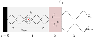
Figure 1: Scheme of the cavity. The fractionally transparent mirror [region (2)] is modeled by a dielectric plate. The active sources are in region 1, which can also contain some medium.

For the sake of transparency, let us consider a one-dimensional cavity modeled by a planar dielectric 4-layer system (Fig. 1). In particular, the layers $j$ $\!=$ $\!0$ and $j$ $\!=$ $\!2$, respectively, are assumed to correspond to perfectly and fractionally reflecting mirrors which confine the cavity (layer $j$ $\!=$ $\!1$). In what follows we use, with respect to $z$, shifted coordinate systems such that $0$ $\!<$ $\!z$ $\!<$ $\!l$ for $j$ $\!=$ $\!1$, $0$ $\!<$ $\!z$ $\!<$ $\!d$ for $j$ $\!=$ $\!2$, and $0$ $\!<$ $\!z$ $\!<\infty$ for $j$ $\!=$ $\!3$. Applying the one-dimensional version of Eq. (II.1) together with Eqs. (15)–(II.1) to the field in the $j$th layer of permittivity $\varepsilon_{j}(\omega)$ ($j$ $\!=$ $\!1,2,3$), we may write

$$\underline{\hat{E}}{{}^{(j)}}(z,\omega,t)=\underline{\hat{E}}^{(j)}_{\mathrm{free}}(z,\omega,t)+\underline{\hat{E}}^{(j)}_{\mathrm{s}}(z,\omega,t),$$ (18)

with

$$\underline{\hat{E}}^{(j)}_{\mathrm{free}}(z,\omega,t)=i\omega\mu_{0}$$

$$\hskip 8.61108pt\times\sum_{j^{\prime}=1}^{3}\int_{[j^{\prime}]}\mbox{\rm d}z^{\prime}\,G^{(jj^{\prime})}(z,z^{\prime},\omega)\underline{\hat{j}}^{(j^{\prime})}_{\mathrm{free}}(z^{\prime},\omega,t)$$ (19)

and

$$\underline{\hat{E}}^{(j)}_{\mathrm{s}}(z,\omega,t)=\frac{i}{\pi\epsilon_{0}\mathcal{A}}\,\frac{\omega^{2}}{c^{2}}\sum_{A}\int\mbox{\rm d}t^{\prime}\,\Theta(t-t^{\prime})$$

$$\hskip 34.44434pt\times\,e^{-i\omega(t-t^{\prime})}\hat{d}_{A}(t^{\prime})\,\mathrm{Im}\,G^{(1j)}(z_{A},z,\omega)$$ (20)

($\mathcal{A}$, mirror area), where the integral relation (157) has been employed. Here, $[j^{\prime}]$ indicates integration over the $j^{\prime}$th layer, the abbreviating notation

$$\underline{\hat{j}}^{(j)}_{\mathrm{free}}(z,\omega,t)=\omega\,\sqrt{\frac{\hbar\epsilon_{0}}{\pi{\cal A}}\,\varepsilon^{\prime\prime}_{j}(\omega)}\,\hat{f}^{(j)}_{\mathrm{free}}(z,\omega,t)$$ (21)

is used, and it is assumed that the active atomic sources are localized inside the cavity. The (nonlocal part of the) Green function reads Khanbekyan et al. (2003)

$$G^{(jj^{\prime})}(z,z^{\prime},\omega)$$

$$\hskip 8.61108pt={\textstyle\frac{1}{2}}i\bigl{[}\mathcal{E}^{(j)>}(z,\omega)\,\Xi^{jj^{\prime}}\mathcal{E}^{(j^{\prime})<}(z^{\prime},\omega)\Theta(j-j^{\prime})$$

$$\hskip 17.22217pt+\mathcal{E}^{(j)<}(z,\omega)\,\Xi^{j^{\prime}j}\mathcal{E}^{(j^{\prime})>}(z^{\prime},\omega)\Theta(j^{\prime}-j)\bigr{]},$$ (22)

where the functions

$$\mathcal{E}^{(j)>}(z,\omega)=e^{i\beta_{j}(z-d_{j})}+r_{j/3}e^{-i\beta_{j}(z-d_{j})}$$ (23)

and

$${\mathcal{E}}^{(j)<}(z,\omega)\,=\,e^{-i\beta_{j}z}+r_{j/0}e^{i\beta_{j}z},$$ (24)

respectively, represent waves of unit strength traveling rightward and leftward in the $j$th layer and being reflected at the boundary [note that $\Theta(j$ $\!-$ $\!j^{\prime})$ means $\Theta(z$ $\!-$ $\!z^{\prime})$ for $j$ $\!=$ $\!j^{\prime}$]. Further, $\Xi^{jj^{\prime}}$ is defined by

$$\Xi^{jj^{\prime}}=\frac{1}{\beta_{3}t_{0/3}}\,\frac{t_{0/j}e^{i\beta_{j}d_{j}}}{D_{j}}\,\frac{t_{3/j^{\prime}}e^{i\beta_{j^{\prime}}d_{j^{\prime}}}}{D_{j^{\prime}}}\,,$$ (25)

where

$$D_{j}=1-r_{j/0}r_{j/3}e^{2i\beta_{j}d_{j}}$$ (26)

and

$$\beta_{j} \equiv\beta_{j}(\omega)=\sqrt{\varepsilon_{j}(\omega)}\,\frac{\omega}{c}$$

$$=[n_{j}^{\prime}(\omega)+in_{j}^{\prime\prime}(\omega)]\,\frac{\omega}{c}=\beta_{j}^{\prime}+i\beta_{j}^{\prime\prime}\quad(\beta_{j}^{\prime},\beta_{j}^{\prime\prime}\geq 0)$$ (27)

($d_{1}$ $\!=$ $\!l$, $d_{2}$ $\!=$ $\!d$, $d_{3}$ $\!=$ $\!0$). The quantities $t_{j/j^{\prime}}$ $\!=$ $\!(\beta_{j}/\beta_{j^{\prime}})t_{j^{\prime}/j}$ and $r_{j/j^{\prime}}$ denote, respectively, the transmission and reflection coefficients between the layers $j^{\prime}$ and $j$, which can be recursively determined (for recursion formulas, see Appendix A).

III Cavity Field

To further evaluate the equations given above, we first consider the field inside the cavity ($j$ $\!=$ $\!1$). In order to make contact with the familiar standing-wave expansion in the idealized case of a lossless cavity, it is useful to rewrite the equations with the aim to obtain a nonmonochromatic mode expansion that takes into account the finite line widths due to the wanted input-output coupling and the unwanted absorption losses that unavoidably exist in practice.

III.1 Nonmonochromatic mode expansion

We begin with the free field. From Eqs. (II.2) and (II.2) it follows that $\underline{\hat{E}}^{(1)}_{\mathrm{free}}(z,\omega,t)$ can be represented in the form of

$$\underline{\hat{E}}_{\mathrm{free}}^{(1)}(z,\omega,t)=$$

$$\hskip 4.30554pt\frac{1}{D_{1}}\left[e^{i\beta_{1}z}\!+\!r_{13}e^{-i\beta_{1}(z-2l)}\right]\left[\hat{C}^{(1)}_{<+}(z,\omega,t)\!-\!\hat{C}^{(1)}_{<-}(z,\omega,t)\right]$$

$$\hskip 12.91663pt-\,\frac{2i\sin(\beta_{1}z)}{D_{1}}\Bigl{\{}\hat{C}^{(1)}_{>-}(z,\omega,t)+r_{13}e^{2i\beta_{1}l}\hat{C}^{(1)}_{>+}(z,\omega,t)$$

$$\hskip 43.05542pt+\,\frac{t_{21}e^{i\beta_{1}l}}{D_{2}^{\prime}}\,\left[\hat{C}^{(2)}_{-}(\omega,t)+r_{23}e^{2i\beta_{2}d}\hat{C}^{(2)}_{+}(\omega,t)\right]$$

$$\hskip 43.05542pt+\,t_{31}e^{i\beta_{1}l}\hat{C}^{(3)}_{-}(\omega,t)\Bigr{\}},$$ (28)

where

$$\hat{C}^{(1)}_{<\pm}(z,\omega,t)$$

$$\hskip 8.61108pt=-\frac{\mu_{0}c}{2n_{1}}\int_{[1]}\mbox{\rm d}z^{\prime}\,\Theta(z\!-\!z^{\prime})e^{\mp i\beta_{1}z^{\prime}}\underline{\hat{j}}^{(1)}_{\mathrm{free}}(z^{\prime},\omega,t),$$ (29)

$$\hat{C}^{(1)}_{>\pm}(z,\omega,t)$$

$$\hskip 8.61108pt=-\frac{\mu_{0}c}{2n_{1}}\int_{[1]}\mbox{\rm d}z^{\prime}\,\Theta(z^{\prime}\!-\!z)e^{\mp i\beta_{1}z^{\prime}}\underline{\hat{j}}^{(1)}_{\mathrm{free}}(z^{\prime},\omega,t),$$ (30)

$$\hat{C}^{(2)}_{\pm}(\omega,t)=-\frac{\mu_{0}c}{2n_{2}}\int_{[2]}\mbox{\rm d}z^{\prime}\,e^{\mp i\beta_{2}z^{\prime}}\underline{\hat{j}}^{(2)}_{\mathrm{free}}(z^{\prime},\omega,t),$$ (31)

$$\hat{C}^{(3)}_{-}(\omega,t)=-\frac{\mu_{0}c}{2n_{3}}\int_{[3]}\mbox{\rm d}z^{\prime}\,e^{i\beta_{3}z^{\prime}}\underline{\hat{j}}^{(3)}_{\mathrm{free}}(z^{\prime},\omega,t),$$ (32)

and

$$D_{2}^{\prime}(\omega)=1-r_{21}r_{23}e^{2i\beta_{2}d}.$$ (33)

Inspection of Eq. (III.1) shows that the function $D_{1}(\omega)$ defined by Eq. (26) for $j=1$ characterizes the spectral response of the cavity. In particular, its zeros determine the (complex) resonance frequencies $\Omega_{k}$,

$$D_{1}(\Omega_{k})=1+r_{13}(\Omega_{k})e^{2i\beta_{1}(\Omega_{k})l}=0.$$ (34)

Note that when the coupling mirror is not a single plate but—as in practice—a multilayer system, then $r_{13}(\omega)$ is the reflection coefficient of the multilayer system and Eq. (34) applies as well. Decomposing $\Omega_{k}$ into real and imaginary parts according to

$$\Omega_{k}=\omega_{k}-{\textstyle\frac{1}{2}}i\Gamma_{k},$$ (35)

we can write the formal solution to Eq. (34) in the form of

$$\omega_{k} =\frac{c}{l}\frac{1}{2|n_{1}|^{2}}$$

$$\quad\times\biggl{\{}\!n_{1}^{\prime}\biggl{[}2\pi k\!+\!\pi\!-\!\tan^{-1}\!\biggl{(}\frac{r_{13}^{\prime\prime}}{r_{13}^{\prime}}\biggr{)}\!\biggr{]}\!-\!n_{1}^{\prime\prime}\ln|r_{13}|\!\biggr{\}}$$ (36)

and

$$\Gamma_{k} =\frac{c}{l}\frac{1}{|n_{1}|^{2}}$$

$$\quad\times\biggr{\{}\!n_{1}^{\prime\prime}\biggl{[}2\pi k\!+\!\pi\!-\tan^{-1}\!\biggl{(}\frac{r_{13}^{\prime\prime}}{r_{13}^{\prime}}\biggr{)}\!\biggr{]}\!+\!n_{1}^{\prime}\ln|r_{13}|\!\biggr{\}}$$ (37)

[$n_{1}$ $\!=$ $\!n_{1}(\Omega_{k})$, $r_{13}$ $\!=$ $\!r_{13}(\Omega_{k})$], from which $\omega_{k}$ and $\Gamma_{k}$ may be calculated by iteration, by starting, e.g., with the resonance frequencies of the lossless cavity.

Let $s(t)$ be a function of time whose Fourier transform is given by

$$\underline{s}(\omega)=\frac{S(\omega)}{D_{1}(\omega)}=\int\mathrm{d}t\,e^{i\omega t}s(t)$$ (38)

and assume that $S(\omega)$ is analytic in the lower half-plane. Employing the residue theorem, we may write

$$s(t)=\!\int\!\frac{\mathrm{d}\omega}{2\pi}\,e^{-i\omega t}\frac{S(\omega)}{D_{1}(\omega)}=\sum_{k}\frac{c}{2n_{1}l}\,\Theta(t)e^{-i\Omega_{k}t}S(\Omega_{k}).$$ (39)

Applying Eqs. (38) and (39) to the $c$-number functions $\sin(\beta_{1}z)D^{-1}$, $\sin(\beta_{1}z)r_{13}e^{2i\beta_{1}l}D^{-1}$, and $[e^{i\beta_{1}z}$ $\!+$ $\!r_{13}e^{-i\beta_{1}(z-2l)}]D^{-1}$ in Eq. (III.1) and disregarding (irrelevant high-frequency) contributions that may arise from poles other than those of $D_{1}^{-1}(\omega)$, we may rewrite $\underline{\hat{E}}_{\mathrm{free}}^{(1)}(z,\omega,t)$ as

$$\underline{\hat{E}}_{\mathrm{free}}^{(1)}(z,\omega,t)=\sum_{k}\underline{\hat{E}}_{k\mathrm{free}}^{(1)}(z,\omega,t),$$ (40)

with

$$\underline{\hat{E}}_{k\mathrm{free}}^{(1)}(z,\omega,t)=i\sqrt{\frac{\mu_{0}c\hbar\omega}{\pi\mathcal{A}n_{1}}}\frac{c}{2n_{1}\!(\Omega_{k})l}\,\sin[\beta_{1}\!(\Omega_{k})z]$$

$$\hskip 8.61108pt\times\,\int\mbox{\rm d}t^{\prime}\,e^{-i\Omega_{k}(t-t^{\prime})}\Theta(t-t^{\prime})$$

$$\hskip 30.1388pt\times\,\Bigl{[}T(\omega)\hat{b}_{\mathrm{in}}(\omega,t^{\prime})+\sum_{\lambda}A_{\lambda}(\omega)\hat{c}_{\lambda}\!(\omega,t^{\prime})\Bigr{]}$$ (41)

($\lambda$ $\!=$ $\!\mathrm{cav},+,-$), where the operators $\hat{c}_{\lambda}(\omega,t)$ are defined according to

$$\hat{c}_{\mathrm{cav}}(\omega,t)=-\alpha_{\mathrm{cav}}\sqrt{\frac{\pi\mathcal{A}}{\mu_{0}c\hbar\omega}}\frac{\mu_{0}c}{2n_{1}}$$

$$\hskip 51.6665pt\times\,\int_{[1]}\mbox{\rm d}z\,\sin(\beta_{1}z)\underline{\hat{j}}^{(1)}_{\mathrm{free}}(z,\omega,t),$$ (42)

$$\hat{c}_{\pm}(\omega,t)=\alpha_{\pm}\sqrt{\frac{\pi\mathcal{A}}{\mu_{0}c\hbar\omega}}$$

$$\hskip 51.6665pt\times\,\left[e^{i\beta_{2}d}\hat{C}^{(2)}_{+}(\omega,t)\pm\hat{C}^{(2)}_{-}(\omega,t)\right],$$ (43)

$$\hat{b}_{\mathrm{in}}(\omega,t)=\frac{2|n_{3}|}{\sqrt{n_{3}^{\prime}}}\sqrt{\frac{\pi\mathcal{A}}{\mu_{0}c\hbar\omega}}\,\hat{C}^{(3)}_{-}(\omega,t),$$ (44)

with

$$\alpha_{\mathrm{cav}} =\alpha_{\mathrm{cav}}(\omega)$$

$$=2\sqrt{2}|n_{1}|\left[n_{1}^{\prime}\sinh(2\beta_{1}^{\prime\prime}l)-n_{1}^{\prime\prime}\sin(2\beta_{1}^{\prime}l)\right]^{-\frac{1}{2}},$$ (45)

$$\alpha_{\pm} =\alpha_{\pm}(\omega)$$

$$=|n_{2}|e^{\beta_{2}^{\prime\prime}d/2}\left[n_{2}^{\prime}\sinh(\beta_{2}^{\prime\prime}d)\pm n_{2}^{\prime\prime}\sin(\beta_{2}^{\prime}d)\right]^{-\frac{1}{2}},$$ (46)

$$A_{\mathrm{cav}}(\omega)=-4i\,\frac{\sqrt{n_{1}}}{\alpha_{\mathrm{cav}}},$$ (47)

$$A_{\pm}(\omega)=-\frac{t_{21}\sqrt{n_{1}}}{D_{2}^{\prime}\alpha_{\pm}}\left(r_{23}e^{i\beta_{2}d}\pm 1\right)e^{i\beta_{1}l},$$ (48)

$$T(\omega)=-\frac{t_{31}\sqrt{n_{1}n_{3}^{\prime}}}{|n_{3}|}\,e^{i\beta_{1}l}.$$ (49)

It is straightforward to prove that the operators $\hat{c}_{\lambda}(\omega,t)$ satisfy Bose commutation relations:

$$\bigl{[}\hat{c}_{\lambda}(\omega,t),\hat{c}_{\lambda^{\prime}}^{\dagger}(\omega^{\prime},t^{\prime})\bigr{]}=\delta_{\lambda\lambda^{\prime}}\delta(\omega-\omega^{\prime})e^{-i\omega(t-t^{\prime})},$$ (50)

$$\bigl{[}\hat{b}_{\mathrm{in}}(\omega,t),\hat{b}_{\mathrm{in}}^{\dagger}(\omega^{\prime},t^{\prime})\bigr{]}=\delta(\omega-\omega^{\prime})e^{-i\omega(t-t^{\prime})},$$ (51)

with all other commutators being zero.

To calculate the electric free field

$$\hat{E}_{\mathrm{free}}^{(1)}(z,t)=\int_{0}^{\infty}\mathrm{d}\omega\,\underline{\hat{E}}_{\mathrm{free}}^{(1)}(z,\omega,t)+\mathrm{H.c.}$$ (52)

[cf. Eq. (10)], we subdivide the $\omega$ axis into intervals $(\Delta_{k})$ $\!\equiv$ $[\frac{1}{2}(\omega_{k-1}$ $\!+$ $\!\omega_{k}),\frac{1}{2}(\omega_{k}$ $\!+$ $\!\omega_{k+1})]$ and write

$$\hat{E}_{\mathrm{free}}^{(1)}(z,t)=\sum_{k}\hat{E}_{k\mathrm{free}}^{(1)}(z,t)+\mathrm{H.c.},$$ (53)

where

$$\hat{E}_{k\mathrm{free}}^{(1)}(z,t)=\int_{(\Delta_{k})}\mbox{\rm d}\omega\,\underline{\hat{E}}_{\mathrm{free}}^{(1)}(z,\omega,t)$$ (54)

(recall that the index $k$ is used to numerate the resonances of the cavity). Substitution of Eq. (40) together with Eq. (III.1) into Eq. (54) yields

$$\hat{E}_{k\mathrm{free}}^{(1)}(z,t)= \int_{(\Delta_{k})}\mbox{\rm d}\omega\,\underline{\hat{E}}_{k\mathrm{free}}^{(1)}(z,\omega,t)$$

$$+\sum_{k^{\prime}\neq k}\int_{(\Delta_{k})}\mbox{\rm d}\omega\,\underline{\hat{E}}_{k^{\prime}\mathrm{free}}^{(1)}(z,\omega,t).$$ (55)

For sufficiently high-$Q$ cavities, i.e., $\Gamma_{k}$ $\!\ll$ $\!\Delta\omega_{k}$, with $\Delta\omega_{k}$ $\!=$ $\!\frac{1}{2}(\omega_{k+1}$ $\!-$ $\!\omega_{k-1})$ being the width of the $k$th interval, the second term in Eq. (III.1) can be regarded as being small compared with the first one and may be omitted in general, leading to

$$\hat{E}^{(1)}_{k\mathrm{free}}(z,t)=\int_{(\Delta_{k})}\mbox{\rm d}\omega\,\underline{\hat{E}}_{k\mathrm{free}}^{(1)}(z,\omega,t).$$ (56)

In this approximation, Eq. (53) reduces to

$$\hat{E}_{\mathrm{free}}^{(1)}(z,t)=\sum_{k}\int_{(\Delta_{k})}\mbox{\rm d}\omega\,\underline{\hat{E}}_{k\mathrm{free}}^{(1)}(z,\omega,t).$$ (57)

Note that within the approximation scheme used, the lower (upper) limit of integration in Eq. (57) may be extended to $-\infty$ ($+\infty$).

To determine the source field

$$\hat{E}_{\mathrm{s}}^{(1)}(z,t)=\int_{0}^{\infty}\mathrm{d}\omega\,\underline{\hat{E}}_{\mathrm{s}}^{(1)}(z,\omega,t)+\mathrm{H.c.},$$ (58)

we start with Eq. (II.2) together with Eq. (II.2). Performing the Fourier transformation and using the resonance properties of the cavity response function [see Eqs. (34)–(39)], we obtain, in the same approximation that leads from Eq. (52) to Eq. (57),

$$\hat{E}_{\mathrm{s}}^{(1)}(z,t)=\sum_{k}\hat{E}_{k\mathrm{s}}^{(1)}(z,t)+\mathrm{H.c.},$$ (59)

where

$$\hat{E}^{(1)}_{k\mathrm{s}}(z,t)=\frac{i\omega_{k}\sin[\beta_{1}(\Omega_{k})z]}{\epsilon_{0}\varepsilon_{1}\!(\Omega_{k})l\mathcal{A}}\sum_{A}\int\!\mbox{\rm d}t^{\prime}\,\Theta(t\!-\!t^{\prime})$$

$$\hskip 25.83325pt\times\,e^{-i\Omega_{k}(t-t^{\prime})}\hat{d}_{A}(t^{\prime})\sin[\beta_{1}\!(\Omega_{k})z_{A}]+\mathrm{H.c.}\,.$$ (60)

Note that in Eq. (III.1) it is assumed that $e^{i\omega_{k}t}\hat{d}_{A}(t)$ may be regarded as being an effectively slowly varying quantity. Combination of $\hat{E}_{\mathrm{free}}^{(1)}(z,t)$ and $\hat{E}_{\mathrm{s}}^{(1)}(z,t)$ to the full intracavity field

$$\hat{E}^{(1)}(z,t)=\hat{E}_{\mathrm{free}}^{(1)}(z,t)+\hat{E}_{\mathrm{s}}^{(1)}(z,t)$$ (61)

yields the nonmonochromatic mode expansion sought.

III.2 Quantum Langevin equations

To bring Eq. (61) [with $\hat{E}_{\mathrm{free}}^{(1)}(z,t)$ from Eq. (57) together with Eq. (III.1) and $\hat{E}_{\mathrm{s}}^{(1)}(z,t)$ from Eq. (59) together with Eq. (III.1)] in a more familiar form, we introduce the operators

$$\hat{c}_{k\lambda}(t)=\frac{1}{\sqrt{2\pi}}\int_{(\Delta_{k})}\mbox{\rm d}\omega\,\hat{c}_{\lambda}(\omega,t),$$ (62)

$$\hat{b}_{k\mathrm{in}}(t)=\frac{1}{\sqrt{2\pi}}\int_{(\Delta_{k})}\mbox{\rm d}\omega\,\hat{b}_{\mathrm{in}}(\omega,t),$$ (63)

which, on a time scale $\Delta t$ $\!\gg$ $\Delta\omega_{k}^{-1},\Delta\omega_{k^{\prime}}^{-1}$, obviously obey [recall Eqs. (50) and (51)] the commutation relations

$$\bigl{[}\hat{c}_{k\lambda}(t),\hat{c}_{k^{\prime}\lambda^{\prime}}^{\dagger}(t^{\prime})\bigr{]}=\delta_{kk^{\prime}}\delta_{\lambda\lambda^{\prime}}\delta(t-t^{\prime}),$$ (64)

$$\bigl{[}\hat{b}_{k\mathrm{in}}(t),\hat{b}_{k^{\prime}\mathrm{in}}^{\dagger}(t^{\prime})\bigr{]}=\delta_{kk^{\prime}}\delta(t-t^{\prime}).$$ (65)

Further, recalling Eqs. (III.1), (57), (59), and (III.1), we may rewrite Eq. (61) as ($\Gamma_{k}$ $\!\ll$ $\!\Delta\omega_{k}$)

$$\hat{E}^{(1)}(z,t)=\sum_{k}E_{k}(z)\hat{a}_{k}(t)+\mathrm{H.c.},$$ (66)

where the standing wave mode functions are defined as

$$E_{k}(z)=i\omega_{k}\left[\frac{\hbar}{\epsilon_{0}\varepsilon_{1}(\omega_{k})l{\cal A}\omega_{k}}\right]^{\frac{1}{2}}\sin[\beta_{1}(\omega_{k})z],$$ (67)

and

$$\hat{a}_{k}(t)=\int\mbox{\rm d}t^{\prime}\,\Theta(t-t^{\prime})e^{-i\Omega_{k}(t-t^{\prime})}$$

$$\hskip 21.52771pt\times\biggl{\{}\biggl{[}\frac{c}{2n_{1}(\omega_{k})l}\biggr{]}^{\frac{1}{2}}\biggl{[}T_{k}\hat{b}_{k\mathrm{in}}(t^{\prime})+\sum_{\lambda}A_{k{\lambda}}\hat{c}_{k{\lambda}}(t^{\prime})\biggr{]}$$

$$\hskip 43.05542pt-\frac{i}{\hbar}\sum_{A}E_{k}(z_{A})\hat{d}_{A}(t^{\prime})\biggr{\}}$$ (68)

[$T_{k}$ $\!=$ $\!T(\omega_{k})$, $A_{k\lambda}$ $\!=$ $\!A_{\lambda}(\omega_{k})$].

From Eq. (III.2) it is not difficult to see that $\hat{a}_{k}$ obeys the Langevin equation

$$\dot{\hat{a}}_{k}(t)=-i\left(\omega_{k}-{\textstyle\frac{1}{2}}i\Gamma_{k}\right)\hat{a}_{k}(t)-\frac{i}{\hbar}\sum_{A}E_{k}(z_{A})\hat{d}_{A}(t)$$

$$\hskip 21.52771pt+\biggl{[}\frac{c}{2n_{1}(\omega_{k})l}\biggr{]}^{\frac{1}{2}}\biggl{[}T_{k}\hat{b}_{k\mathrm{in}}(t)+\sum_{\lambda}A_{k\lambda}\hat{c}_{k\lambda}(t)\biggr{]},$$ (69)

and it can be proved (see Appendix D) that the equal-time commutation relation

$$[\hat{a}_{k}(t),\hat{a}_{k^{\prime}}^{\dagger}(t)]=\delta_{kk^{\prime}}$$ (70)

holds.

The damping rate in the first term on the right-hand side of Eq. (III.2) can be decomposed as follows (see Appendix C):

$$\Gamma_{k}=\gamma_{k\mathrm{rad}}+\gamma_{k\mathrm{abs}}\,,$$ (71)

$$\gamma_{k\mathrm{rad}}=\frac{c}{2|n_{1}(\omega_{k})|l}|T_{k}|^{2},$$ (72)

$$\gamma_{k\mathrm{abs}}=\sum_{\lambda}\gamma_{k\lambda}=\frac{c}{2|n_{1}(\omega_{k})|l}\sum_{\lambda}|A_{k\lambda}|^{2}.$$ (73)

Here, $\gamma_{k\mathrm{rad}}$ is the radiative decay rate describing the transmission losses due to the input-output coupling and $\gamma_{k\mathrm{abs}}$ is the (nonradiative) decay rate describing the absorption losses inside the cavity (term proportional to $|A_{k\mathrm{cav}}|^{2}$) and inside the mirror (terms proportional to $|A_{k\pm}|^{2}$). Accordingly, the Langevin noise force as given by the third term on the right-hand side of Eq. (III.2) consists of the contributions associated with the losses due to the input-output coupling [term proportional to $T_{k}\hat{b}_{k\mathrm{in}}(t)$] and the absorption losses inside the cavity [term proportional to $A_{k\mathrm{cav}}\hat{c}_{k\mathrm{cav}}(t)$] and inside the mirror [terms proportional to $A_{k\pm}\hat{c}_{k\pm}(t)$].

Equation (III.2) can be regarded as a generalization of the results derived in Ref. Knöll et al. (1987) for a leaky cavity without material absorption to a realistic cavity which gives rise to both radiative and unwanted (nonradiative) absorption losses. In particular, when $\varepsilon_{1}(\omega_{k})$ can be regarded as being real, then the second term on the right-hand side of Eq. (III.2) is nothing but the familiar commutator term $(i\hbar)^{-1}[\hat{a}_{k},\hat{H}_{\mathrm{int}}]$, where

$$\hat{H}_{\mathrm{int}}=-\sum_{A}\sum_{k}E_{k}(z_{A})\hat{d}_{A}\hat{a}_{k}+\mathrm{H.c.}.$$ (74)

Moreover, from Eq. (III.2) together with Eqs. (71)–(73) it is seen that the effect of absorption losses on the intracavity field may be equivalently described within the frame of Markovian damping theory, with

$$\hat{H}_{\mathrm{abs,int}}=\hbar\sum_{\lambda}\sum_{k}\!\int_{(\Delta_{k})}\!\!\mbox{\rm d}\omega\,\biggl{[}\frac{c}{2n_{1}(\omega)l}\biggr{]}^{\frac{1}{2}}A_{k\lambda}(\omega)\hat{a}_{k}^{\dagger}\hat{c}_{k\lambda}(\omega)$$

$$\hskip 43.05542pt+\mathrm{H.c.}$$ (75)

being the total interaction energy between the cavity modes and the dissipative systems responsible for absorption. Thus Eq. (III.2) can be also regarded as an extension of the results derived in Ref. Gardiner and Collett (1985) within the frame of quantum noise theories, by adding to the Hamiltonian therein an interaction energy of the type (III.2). Needless to say that also other than the dissipative channels considered here can be included in the interaction energy. The unwanted losses attributed to the cavity wall that has been assumed to be perfectly reflecting is a typical example. Note that Eq. (III.2) implies that each cavity mode is coupled to its own dissipative systems.

IV Field outside the cavity

Once the cavity field is expressed in terms of nonmonochromatic mode operators $\hat{a}_{k}(t)$, the question arises of how the outgoing field is related to it. To answer, we first rewrite the outgoing field using Eqs. (18)–(II.2) with $j$ $\!=$ $\!3$ and proceed similarly as in the case of the cavity field.

IV.1 Outgoing field

We again begin with the free field. Inserting the Green tensor as given by Eq. (II.2) in Eq. (II.2) ($j$ $\!=$ $\!3$) and separating the incoming and outgoing parts propagating along $-z$ and $z$, respectively, we may represent the outgoing part at $z$ $\!=$ $\!0^{+}$ (cf. Fig. 1) as follows (see Appendix B):

$$\underline{\hat{E}}_{{\rm out},{\rm free}}^{(3)}(z,\omega,t)\bigr{|}_{z=0^{+}}$$

$$=\frac{t_{13}e^{i\beta_{1}l}}{D_{1}}\biggl{\{}\left[\hat{C}^{(1)}_{<+}(l,\omega,t)-\hat{C}^{(1)}_{<-}(l,\omega,t)\right]$$

$$\hskip 21.52771pt-\frac{t_{21}e^{i\beta_{1}l}}{D_{2}^{\prime}}\left[r_{23}e^{2i\beta_{2}d}\hat{C}^{(2)}_{+}(\omega,t)+\hat{C}^{(2)}_{-}(\omega,t)\right]$$

$$\hskip 120.55518pt-\,t_{31}e^{i\beta_{1}l}\hat{C}^{(3)}_{-}(\omega,t)\biggr{\}}$$

$$+\,\frac{t_{23}e^{i\beta_{2}d}}{D_{2}^{\prime}}\left[\hat{C}^{(2)}_{+}(\omega,t)+r_{21}\hat{C}^{(2)}_{-}(\omega,t)\right]\!+\!r_{31}\hat{C}^{(3)}_{-}(\omega,t),$$ (76)

where $\hat{C}^{(1)}_{<\pm}(l,\omega,t)$ is defined by Eq. (III.1) (for $x$ $\!=$ $\!l$), and $\hat{C}^{(2)}_{\pm}(\omega,t)$ and $\hat{C}^{(3)}_{-}(\omega,t)$ are defined by Eqs. (31) and (32), respectively. Treating the term $D_{1}^{-1}(\omega)$ in the same way as that leading from Eq. (III.1) to Eq. (40) together with Eqs. (III.1)–(III.1), from Eq. (IV.1) we derive

$$\underline{\hat{E}}_{{\rm out},{\rm free}}^{(3)}(z,\omega,t)\bigr{|}_{z=0^{+}}=\sum_{k}\underline{\hat{E}}_{k\mathrm{out},{\rm free}}^{(3)}(z,\omega,t)\bigr{|}_{z=0^{+}},$$ (77)

where

$$\underline{\hat{E}}_{k\mathrm{out},{\rm free}}^{(3)}(z,\omega,t)\bigr{|}_{z=0^{+}}=\frac{1}{2}\sqrt{\frac{\mu_{0}c\hbar\omega}{\pi\mathcal{A}n_{1}}}\frac{c}{2n_{1}\!(\Omega_{k})l}\,t_{13}$$

$$\hskip 17.22217pt\times\,\int\mbox{\rm d}t^{\prime}e^{-i\Omega_{k}(t-t^{\prime})}\Theta(t-t^{\prime})\,e^{i\beta_{1}l}$$

$$\hskip 25.83325pt\times\,\biggl{[}T(\omega)\hat{b}_{\mathrm{in}}(\omega,t^{\prime})+\sum_{\lambda}A_{\lambda}(\omega)\hat{c}_{\lambda}\!(\omega,t^{\prime})\biggr{]}$$

$$\hskip 8.61108pt+\frac{1}{2}\,\sqrt{\frac{\mu_{0}c\hbar\omega}{\pi\mathcal{A}}}\,\biggl{\{}\frac{\sqrt{n_{3}^{\prime}}r_{31}}{|n_{3}|}\,\hat{b}_{k\mathrm{in}}(\omega,t)$$

$$\hskip 25.83325pt+\frac{t_{23}}{D_{2}^{\prime}}\biggl{[}\frac{r_{21}e^{i\beta_{2}d}+1}{\alpha_{+}}\,\hat{c}_{k+}(\omega,t)$$

$$\hskip 64.58313pt-\frac{r_{21}e^{i\beta_{2}d}-1}{\alpha_{-}}\,\hat{c}_{k-}(\omega,t)\biggr{]}\biggr{\}}.$$ (78)

As we see from this equation, there are three physically different contributions to the outgoing free field. The first (integral) term proportional to $t_{13}$ represents the fraction of the cavity field transmitted through the mirror [cf. Eq. (III.1)]. The term proportional to $r_{31}\hat{b}_{k\mathrm{in}}(\omega,t)$ represents the reflected part of the incoming field, whereas the terms proportional to $t_{23}\hat{c}_{k\pm}(\omega,t)$ describe the field attributed to the noise sources inside the mirror.

Integrating Eq. (IV.1) with respect to $\omega$, we obtain the free-field part of the outgoing electric field in the time-domain,

$$\hat{E}_{{\rm out},{\rm free}}^{(3)}(z,t)\bigr{|}_{z=0^{+}}=\sum_{k}\hat{E}_{k{\rm out},{\rm free}}^{(3)}(z,t)\bigr{|}_{z=0^{+}}+\mathrm{H.c.}$$ (79)

[cf. Eqs. (52) and (53)], where, within the approximation scheme used,

$$\hat{E}_{k{\rm out},{\rm free}}^{(3)}(z,t)\bigr{|}_{z=0^{+}}=\int_{(\Delta_{k})}\mbox{\rm d}\omega\,\underline{\hat{E}}_{k{\rm out},{\rm free}}^{(3)}(z,\omega,t)\bigr{|}_{z=0^{+}}$$ (80)

[cf. Eqs. (53)–(57)].

Starting from Eq. (II.2) ($j$ $\!=$ $\!3$) together with Eq. (II.2), we may rewrite the source-field part of the outgoing electric field to obtain, in close analogy to Eqs. (58) and (III.1),

$$\hat{E}_{{\rm out},{\rm s}}^{(3)}(z,t)\bigr{|}_{z=0^{+}} =\hat{E}_{{\rm s}}^{(3)}(z,t)\bigl{|}_{z=0^{+}}$$

$$=\sum_{k}\hat{E}_{k,{\rm s}}^{(3)}(z,t)\bigr{|}_{z=0^{+}}+\mathrm{H.c.},$$ (81)

where

$$\hat{E}^{(3)}_{k\mathrm{s}}(z,t)\bigr{|}_{z=0^{+}}=\int_{(\Delta_{k})}\!\mbox{\rm d}\omega\,\underline{\hat{E}}^{(3)}_{k\mathrm{s}}(z,\omega,t)\bigr{|}_{z=0^{+}}+\mathrm{H.c.}$$

$$\hskip 8.61108pt=\frac{\omega_{k}t_{13}\exp[i\beta_{1}(\Omega_{k})l]}{2\epsilon_{0}\varepsilon_{1}(\Omega_{k})l\mathcal{A}}\sum_{A}\int\mbox{\rm d}t^{\prime}\,\Theta(t-t^{\prime})$$

$$\hskip 25.83325pt\times\,e^{-i\Omega_{k}(t-t^{\prime})}\hat{d}_{A}(t^{\prime})\sin[\beta_{1}(\Omega_{k})z_{A}]+\mathrm{H.c.}.$$ (82)

Finally, combination of the free-field part and the source-field part yields the full outgoing field at $z$ $\!=$ $\!0^{+}$,

$$\hat{E}_{\mathrm{out}}^{(3)}(z,t)\bigr{|}_{z=0^{+}}=\hat{E}_{\mathrm{out,free}}^{(3)}(z,t)\bigr{|}_{z=0^{+}}+\hat{E}_{\mathrm{s}}^{(3)}(z,t)\bigr{|}_{z=0^{+}}.$$ (83)

IV.2 Global input-output relation

Let us restrict our attention, for simplicity, to a cavity in free space, i.e., $n_{3}\to 1$, and define the operators

$$\hat{b}_{\mathrm{out}}(\omega,t)=2\sqrt{\frac{\pi\mathcal{A}}{\mu_{0}c\hbar\omega}}\,\underline{\hat{E}}^{(3)}_{\mathrm{out}}(z,\omega,t)\bigr{|}_{z=0^{+}}.$$ (84)

By using the formulas given in Section IV.1 it is not difficult to see that we may rewrite the $\omega$-integrated operator

$$\hat{b}_{\mathrm{out}}(t)=\frac{1}{\sqrt{2\pi}}\int\mathrm{d}\omega\,\hat{b}_{\mathrm{out}}(\omega,t)$$ (85)

as

$$\hat{b}_{\mathrm{out}}(t)=\sum_{k}\hat{b}_{k\mathrm{out}}(t),$$ (86)

where

$$\hat{b}_{k\mathrm{out}}(t)=\frac{1}{\sqrt{2\pi}}\int_{(\Delta_{k})}\mathrm{d}\omega\,\hat{b}_{k\mathrm{out}}(\omega,t),$$ (87)

with $\hat{b}_{k\mathrm{out}}(\omega,t)$ being given by

$$\hat{b}_{k\mathrm{out}}(\omega,t)=2\sqrt{\frac{\pi\mathcal{A}}{\mu_{0}c\hbar\omega}}\,\underline{\hat{E}}^{(3)}_{ks}(z,\omega,t)\bigr{|}_{z=0^{+}}$$

$$\hskip 4.30554pt+\frac{c}{2n_{1}l}\,T_{k}^{({\rm o})}(\omega)\int\mbox{\rm d}t^{\prime}\,\Theta(t-t^{\prime})e^{-i\Omega_{k}(t-t^{\prime})}$$

$$\hskip 25.83325pt\times\,\biggl{[}T_{k}(\omega)\hat{b}_{k\mathrm{in}}(\omega,t^{\prime})+\sum_{\lambda}A_{k\lambda}(\omega)\hat{c}_{k\lambda}\!(\omega,t^{\prime})\biggr{]}$$

$$\hskip 4.30554pt+A_{k+}^{({\rm o})}(\omega)\hat{c}_{k+}(\omega,t)+A_{k-}^{({\rm o})}(\omega)\hat{c}_{k-}(\omega,t)$$

$$\hskip 4.30554pt+R_{k}^{({\rm o})}(\omega)\hat{b}_{k\mathrm{in}}(\omega,t).$$ (88)

Here, the functions $A_{k\pm}^{\mathrm{(o)}}(\omega)$, $R_{k}^{\mathrm{(o)}}(\omega)$, and $T_{k}^{\mathrm{(o)}}(\omega)$ are defined as follows:

$$A_{k\pm}^{({\rm o})}(\omega)=\frac{t_{23}}{D_{2}^{\prime}}\frac{1\pm r_{21}e^{i\beta_{2}d}}{\alpha_{\pm}}\,,$$ (89)

$$T_{k}^{({\rm o})}(\omega)=\frac{t_{13}}{\sqrt{n_{1}}}\,e^{i\beta_{1}l},$$ (90)

$$R_{k}^{({\rm o})}(\omega)=r_{31}.$$ (91)

Performing in Eq. (87) the $\omega$ integral, on extending again the lower (upper) limit to $-\infty$ ($+\infty$) and recalling Eqs. (III.2) and (IV.1), we see that the source term in Eq. (IV.2) and the second (integral) term in this equation sum up to a term proportional to the cavity-field operator $\hat{a}_{k}(t)$. Thus, from Eqs. (86)–(IV.2) it follows that ($\Gamma_{k}$ $\!\ll$ $\!\Delta\omega_{k}$)

$$\hat{b}_{k\mathrm{out}}(t)= \left[\frac{c}{2n_{1}(\omega_{k})l}\right]^{\frac{1}{2}}T_{k}^{({\rm o})}\hat{a}_{k}(t)+R_{k}^{({\rm o})}\hat{b}_{k\mathrm{in}}(t)$$

$$+A_{k+}^{({\rm o})}\hat{c}_{k+}(t)+A_{k-}^{({\rm o})}\hat{c}_{k-}(t)$$ (92)

[$T_{k}^{({\rm o})}$ $\!=$ $\!T_{k}^{({\rm o})}(\omega_{k})$, $A^{({\rm o})}_{k\pm}$ $\!=$ $\!A^{({\rm o})}_{k\pm}(\omega_{k})$, $R_{k}^{({\rm o})}$ $\!=$ $\!R_{k}^{({\rm o})}(\omega_{k})$].

If on the right-hand side in Eq. (IV.2) the third term and the forth term, which result from the absorption losses in the coupling mirror, are omitted, then Eq. (IV.2) reduces to the well-known input-output relation Gardiner and Collett (1985); Knöll et al. (1987) for a leaky cavity whose losses solely result from the wanted radiative input-output coupling, in which case $|R_{k}^{({\rm o})}(\omega_{k})|$ $\!=$ $\!1$ holds. It can be shown that the operators that appear in Eq. (IV.2) obey commutation relations of the type given in Ref. Knöll et al. (1987). In particular on the time scale considered, i.e., $\Delta t$ $\!\gg$ $\Delta\omega_{k}^{-1},\Delta\omega_{k^{\prime}}^{-1}$, the commutation relation

$$\bigl{[}\hat{b}_{k{\rm out}}(t),\hat{b}^{\dagger}_{k^{\prime}{\rm out}}(t^{\prime})\bigr{]}=\delta_{kk^{\prime}}\delta(t-t^{\prime})$$ (93)

holds (see Appendix E).

As we know from Sec. III.2, the damping of the cavity modes due to unwanted losses can simply be described by introducing into the Hamiltonian an interaction energy of the type (III.2) and treating its effect in Markovian approximation. However, since such a simple interaction energy does not allow to include in the theory effects such as for example the influence of the coupling-mirror-assisted absorption on the outgoing field via the incoming field, the last two terms in Eq. (IV.2) are missing and hence $|R_{k}^{\mathrm{(o)}}|$ $\!=$ $\!1$ is set (see, e.g., Ref. Gardiner and Collett (1985)). As a matter of fact, due to unavoidable losses it is always observed that $|R_{k}^{\mathrm{(o)}}|$ $\!<$ $\!1$ in practice. The additional noise associated with these losses is just described by the last two terms in Eq. (IV.2).

The input-output relation (IV.2) can be used, e.g., to calculate correlation functions of the outgoing field in terms of (in general mixed) correlation functions of the cavity field, the incoming field, and the dissipative channels. In what follows we will not consider the one or the other correlation function, but focus on the quantum state as a whole. In this connection it should be stress laid on the fact that Eq. (IV.2) as a global input-output relation does not specify the incoming and outgoing (nonmonochromatic) modes as well as those of the dissipative channels which are really connected in the relevant frequency interval defined by the bandwidth of the cavity mode and hence basically carry the quantum state.

V Quantum state of the outgoing field

For the sake of transparency let us suppose that during the passage of atoms through the cavity the $k$th cavity mode is prepared in some quantum state and assume that the preparation time is sufficiently short compared with the decay time $\Gamma_{k}^{-1}$, so that the two time scales are well distinguishable. In this case we may assume that at some time $t_{0}$ (when the atom leaves the cavity) the cavity mode is prepared in a given quantum state and its evolution in the further course of time (i.e., for times $t$ $\!\geq$ $\!t_{0}$) can be treated as free-field evolution. To specify the relevant modes, it is useful not to use Eq. (IV.2) but return to Eq. (IV.2) and relate therein $\hat{b}_{k\mathrm{out}}(\omega,t)$ to $\hat{a}_{k}(t_{0})$. It can be proved (see Appendix F) that on the (relevant) time scale $\Delta t$ $\!\gg$ $\!\Delta\omega_{k}^{-1}$ Eq. (IV.2) can be rewritten as

$$\hat{b}_{k\mathrm{out}}(\omega,t)$$

$$\hskip 4.30554pt=\,\left[\frac{c}{2n_{1}(\omega_{k})l}\right]^{\frac{1}{2}}T_{k}^{({\rm o})}\,\frac{1}{\sqrt{2\pi}}\int_{t_{0}}^{t+\Delta t}\!\mbox{\rm d}t^{\prime}\,e^{-i\omega(t-t^{\prime})}\hat{a}_{k}(t^{\prime})$$

$$\hskip 8.61108pt+A_{k+}^{({\rm o})}\hat{c}_{k+}(\omega,t_{0})e^{-i\omega(t-t_{0})}+A_{k-}^{({\rm o})}\hat{c}_{k-}(\omega,t_{0})e^{-i\omega(t-t_{0})}$$

$$\hskip 8.61108pt+R_{k}^{({\rm o})}\hat{b}_{k\mathrm{in}}(\omega,t_{0})e^{-i\omega(t-t_{0})}.$$ (94)

Note that integration of both sides of Eq. (V) with respect to $\omega$ over the interval $(\Delta_{k})$ leads to the input-output relation (IV.2) ($n_{3}\to 1$). It should be mentioned that, for the special case of purely radiative losses, an equation of the type of Eq. (V) could be also found from the quantum stochastic theory in Ref. Gardiner and Collett (1985), which would however suggest that its validity only requires the condition $\Delta t$ $\!>$ $\!0$ to be satisfied.

Substituting Eq. (III.2) (for $t$ $\!\geq$ $t_{0}$) together with Eqs. (62) and (63) into Eq. (V), we derive

$$\hat{b}_{k\mathrm{out}}(\omega,t)=F^{*}_{k}(\omega,t)\hat{a}_{k}(t_{0})+\hat{B}_{k}(\omega,t),$$ (95)

where the $c$-number function $F_{k}(\omega,t)$ reads

$$F_{k}(\omega,t) =\frac{i}{\sqrt{2\pi}}\left(\frac{c}{2n_{1}^{*}l}\right)^{1/2}\!T_{k}^{({\rm o})*}\,e^{i\omega(t-t_{0})}$$

$$\quad\times\,\frac{\exp\left[-i(\omega-\Omega^{*}_{k})(t+\Delta t-t_{0})\right]-1}{\omega-\Omega^{*}_{k}}\,,$$ (96)

and the operator $\hat{B}_{k}(\omega,t)$ is a linear functional of the operators $\hat{b}_{k\rm{in}}(\omega,t_{0})$ and $\hat{c}_{k\lambda}(\omega,t_{0})$:

$$\hat{B}_{k}(\omega,t)=\int_{(\Delta_{k})}\!\mbox{\rm d}\omega^{\prime}\,\Bigl{[}G_{k\rm{in}}^{*}(\omega,\omega^{\prime},t)\,\hat{b}_{k\mathrm{in}}(\omega^{\prime},t_{0})\Bigr{.}$$

$$\hskip 21.52771pt\Bigl{.}+\sum_{\lambda}G_{k\lambda}^{*}(\omega,\omega^{\prime},t)\,\hat{c}_{k\lambda}(\omega^{\prime},t_{0})\Bigr{]}.$$ (97)

Here,

$$G_{k\rm{in}}(\omega,\omega^{\prime},t)=T_{k}^{({\rm o})*}T_{k}^{*}\upsilon_{k}(\omega,\omega^{\prime},t)$$

$$\hskip 64.58313pt+R_{k}^{({\rm o})*}e^{i\omega^{\prime}(t-t_{0})}\delta(\omega-\omega^{\prime}),$$ (98)

$$G_{k\rm{cav}}(\omega,\omega^{\prime},t)=T_{k}^{({\rm o})*}A_{k\mathrm{cav}}^{*}\upsilon_{k}(\omega,\omega^{\prime},t),$$ (99)

$$G_{k\pm}(\omega,\omega^{\prime},t)=T_{k}^{({\rm o})*}A^{*}_{k\pm}\upsilon_{k}(\omega,\omega^{\prime},t)$$

$$\hskip 64.58313pt+A^{({\rm o})*}_{k\pm}e^{i\omega^{\prime}(t-t_{0})}\delta(\omega-\omega^{\prime}),$$ (100)

with

$$\upsilon_{k}(\omega,\omega^{\prime},t)=\frac{1}{2\pi}\frac{c}{2n_{1}^{*}l}\frac{e^{-i\omega\Delta t}}{\omega-\Omega_{k}^{*}}$$

$$\hskip 17.22217pt\times\,\left[\frac{e^{i\omega^{\prime}(t+\Delta t-t_{0})}-e^{i\Omega_{k}^{*}(t+\Delta t-t_{0})}}{\omega^{\prime}-\Omega_{k}^{*}}\right.$$

$$\hskip 43.05542pt\left.-\,\frac{e^{i\omega(t+\Delta t-t_{0})}-e^{i\omega^{\prime}(t+\Delta t-t_{0})}}{\omega-\omega^{\prime}}\right].$$ (101)

V.1 Nonmonochromatic modes

To calculate the quantum state of the outgoing field, it is convenient to introduce a unitary, explicitly time-dependent transformation according to

$$\hat{b}_{k\mathrm{out}}(\omega,t)=\sum_{i}\phi_{i}^{*}(\omega,t)\hat{b}_{k\mathrm{out}}^{(i)}(t),$$ (102)

$$\hat{b}_{k\mathrm{out}}^{(i)}(t)=\int_{(\Delta_{k})}\!\mbox{\rm d}\omega\,\phi_{i}(\omega,t)\hat{b}_{k\mathrm{out}}(\omega,t),$$ (103)

where, for chosen $t$, the nonmonochromatic mode functions $\phi_{i}(\omega,t)$ are a complete set of square integrable orthonormal functions:

$$\int_{(\Delta_{k})}\mbox{\rm d}\omega\,\phi_{i}(\omega,t)\phi_{j}^{*}(\omega,t)=\delta_{ij},$$ (104)

$$\sum_{i}\phi_{i}(\omega,t)\phi_{i}^{*}(\omega^{\prime},t)=\delta(\omega-\omega^{\prime}).$$ (105)

Needless to say that the commutation relation

$$\bigl{[}\hat{b}_{k\mathrm{out}}^{(i)}(t),\hat{b}_{k\mathrm{out}}^{(j)\dagger}(t)\bigr{]}=\delta_{ij}$$ (106)

holds.

Let $\hat{b}_{k\mathrm{out}}^{(1)}(t)$ be the operator attributed to the outgoing mode that is related to the cavity mode through the input-output relation (95):

$$\phi_{1}(\omega,t)=\frac{F_{k}(\omega,t)}{\sqrt{\eta_{k}(t)}}\,,$$ (107)

$$\eta_{k}(t)=\int_{(\Delta_{k})}\mbox{\rm d}\omega\,|F_{k}(\omega,t)|^{2}.$$ (108)

By using Eqs. (95), (107), and (108) we may rewrite (for chosen $k$) Eq. (103) as

$$\hat{b}_{k\mathrm{out}}^{(i)}(t)=\left\{\begin{array}[]{ll}\sqrt{\eta_{k}(t)}\,\hat{a}_{k}(t_{0})+\hat{B}_{k}^{(i)}(t)&\ \mathrm{if}\ i=1,\\[8.61108pt] \hat{B}_{k}^{(i)}(t)&\ \mathrm{otherwise},\end{array}\right.$$ (109)

where

$$\hat{B}_{k}^{(i)}(t)=\int_{(\Delta_{k})}\mbox{\rm d}\omega\,\phi_{i}(\omega,t)\hat{B}_{k}(\omega,t).$$ (110)

Inserting Eq. (V) in Eq. (110), we may rewrite $\hat{B}_{k}^{(i)}(t)$ as

$$\hat{B}_{k}^{(i)}(t)=\sqrt{\zeta^{(i)}_{k\mathrm{in}}(t)}\,\hat{b}^{(i)}_{k\mathrm{in}}(t)+\sum_{\lambda}\sqrt{\zeta^{(i)}_{k\lambda}(t)}\,\hat{c}^{(i)}_{k\lambda}(t).$$ (111)

Here the functions $\zeta^{(i)}_{k\sigma}(t)$ ($\sigma$ $\!=$ $\!\mathrm{in},\lambda$) read

$$\zeta^{(i)}_{k\sigma}(t)=\int_{(\Delta_{k})}\mbox{\rm d}\omega\,|\chi^{(i)}_{k\sigma}(\omega,t)|^{2},$$ (112)

where

$$\chi^{(i)}_{k\sigma}(\omega,t)=\int_{(\Delta_{k})}\mbox{\rm d}\omega^{\prime}\,\phi_{i}(\omega^{\prime},t)G_{k\sigma}^{*}(\omega^{\prime},\omega,t).$$ (113)

The operators $\hat{b}^{(i)}_{k\mathrm{in}}(t)$ and $\hat{c}^{(i)}_{k\lambda}(t)$ are defined by

$$\hat{b}^{(i)}_{k\mathrm{in}}(t)=\int_{(\Delta_{k})}\mbox{\rm d}\omega\,\frac{\chi^{(i)}_{k\mathrm{in}}(\omega,t)}{\sqrt{\zeta^{(i)}_{k\mathrm{in}}(t)}}\,\hat{b}_{k\mathrm{in}}(\omega,t_{0}),$$ (114)

$$\hat{c}^{(i)}_{k\lambda}(t)=\int_{(\Delta_{k})}\mbox{\rm d}\omega\,\frac{\chi^{(i)}_{k\lambda}(\omega,t)}{\sqrt{\zeta^{(i)}_{k\lambda}(t)}}\,\hat{c}_{k\lambda}(\omega,t_{0}).$$ (115)

V.2 Phase-space functions

Introducing in the characteristic functional

$$C_{k{\rm out}}[\beta(\omega),t]$$

$$\hskip 8.61108pt=\left\langle\exp\left[\int_{(\Delta_{k})}\!\mbox{\rm d}\omega\,\beta(\omega)\hat{b}^{\dagger}_{k\mathrm{out}}(\omega,t)-\mathrm{H.c.}\right]\right\rangle$$ (116)

the operators $\hat{b}^{(i)}_{k\mathrm{out}}(t)$ according to Eq. (102) and taking into account the commutation relation (106) we see that the operator exponential factorizes as

$$\exp\!\left[\int_{(\Delta_{k})}\mbox{\rm d}\omega\,\beta(\omega)\hat{b}^{\dagger}_{k\mathrm{out}}(\omega,t)-\mathrm{H.c.}\right]$$

$$\hskip 43.05542pt=\prod_{i}\exp\!\left[\beta_{i}\hat{b}^{(i)\dagger}_{k\mathrm{out}}(t)-\mathrm{H.c.}\right],$$ (117)

where

$$\beta_{i}=\beta_{i}(t)=\int_{(\Delta_{k})}\mbox{\rm d}\omega\,\phi_{i}(\omega,t)\beta(\omega).$$ (118)

Let us further consider the case, when the nonmonochromatic modes of the incoming field and dissipative channels corresponding to $\hat{B}_{k}^{(i)}(t)$, $i\neq 1$, are in vacuum state at the initial time $t_{0}$. Then we may assume that the resulting characteristic function factorizes as well, with

$$C_{k{\rm out}}(\beta_{1},t)=\left\langle\exp\!\left[\beta_{1}\hat{b}^{(1)\dagger}_{k\mathrm{out}}(t)-\mathrm{H.c.}\right]\right\rangle$$ (119)

being the characteristic function of the relevant outgoing mode. Using Eq. (109) and noting that the commutation relation

$$\bigl{[}\hat{a}_{k}(t_{0}),\hat{B}_{k}^{(1)\dagger}(t)\bigr{]}=0\quad(t\geq t_{0})$$ (120)

holds (see Appendix G), we may rewrite Eq. (119) as

$$C_{k{\rm out}}(\beta_{1},t)=\left\langle\exp\!\left[\beta_{1}\sqrt{\eta_{k}(t)}\hat{a}_{k}^{\dagger}(t_{0})-\mathrm{H.c.}\right]\right.$$

$$\hskip 73.19421pt\times\,\left.\exp\!\left[\beta_{1}\hat{B}_{k}^{(1)\dagger}(t)-\mathrm{H.c.}\right]\right\rangle.$$ (121)

Noting that according to Eq. (111) $\hat{B}_{k}^{(1)\dagger}(t)$ is a functional of $\hat{b}_{k\mathrm{in}}(\omega,t_{0})$ and $\hat{c}_{k\lambda}(\omega,t_{0})$ and assuming that the density operator (at the initial time $t_{0}$) factorizes with respect to the cavity field, the incoming field, the dissipative channels, we obtain

$$C_{k{\rm out}}(\beta_{1},t)=\left\langle\exp\!\left[\beta_{1}\sqrt{\eta_{k}(t)}\hat{a}_{k}^{\dagger}(t_{0})-\mathrm{H.c.}\right]\right\rangle$$

$$\hskip 73.19421pt\times\,\left\langle\exp\!\left[\beta_{1}\hat{B}_{k}^{(1)\dagger}(t)-\mathrm{H.c.}\right]\right\rangle.$$ (122)

Making use of the commutation relations (70) and

$$\bigl{[}\hat{B}_{k}^{(1)}(t),\hat{B}_{k}^{(1)\dagger}(t)\bigr{]}=1-\eta_{k}(t),$$ (123)

which follows from Eq. (109) together with the commutation relations (70), (106), and (120), the further evaluation of Eq. (V.2) is straightforward. Following Ref. Khanbekyan et al. (2004) and calculating the characteristic function $C_{\mathrm{out}}(\beta,t;s)$ $\!\equiv$ $\!C_{k\mathrm{out}}(\beta_{1},t;s)$ in $s$ order of the quantum state of the relevant outgoing field, we may express it in terms of the characteristic function $C(\beta^{\prime};s^{\prime})$ $\!\equiv$ $\!C_{k}(\beta^{\prime};s^{\prime})$ of the quantum state of the initially excited cavity mode and the characteristic functions $C_{\sigma}(\beta_{\sigma};s_{\sigma})$ $\!\equiv$ $\!C_{k\sigma}(\beta_{\sigma};s_{\sigma})$ of the quantum states of the incoming field ($\sigma$ $\!=$ $\!\mathrm{in}$) and the dissipative channels ($\sigma$ $\!=$ $\!\lambda$) as

$$C_{\mathrm{out}}(\beta,t;s)=e^{-{\textstyle\frac{1}{2}}\xi(t)|\beta|^{2}}C\bigl{[}\sqrt{\eta(t)}\,\beta;s^{\prime}\bigr{]}$$

$$\hskip 77.49976pt\times\,\prod_{\sigma}\!C_{\sigma}\!\Bigl{[}\sqrt{\zeta_{\sigma}(t)}\,\beta;s_{\sigma}\Bigr{]},$$ (124)

where

$$\xi(t)=\eta(t)s^{\prime}+\sum_{\sigma}\zeta_{\sigma}(t)s_{\sigma}-s$$ (125)

[$\eta(t)$ $\!\equiv$ $\!\eta_{k}(t)$, $\zeta_{\sigma}(t)$ $\!\equiv$ $\!\zeta^{(1)}_{k\sigma}(t)$].

From Eq. (V.2) the phase-space function in $s$ order can be derived to be

$$P_{\mathrm{out}}(\alpha,t;s)=\frac{2}{\pi}\frac{1}{\xi(t)}$$

$$\hskip 8.61108pt\times\,\int\mbox{\rm d}^{2}\alpha^{\prime}\,P(\alpha^{\prime};s^{\prime})\prod_{\sigma}\int\mbox{\rm d}^{2}\alpha_{\sigma}\,P_{\sigma}(\alpha_{\sigma};s_{\sigma})$$

$$\hskip 8.61108pt\times\,\exp\biggl{[}-\frac{2}{\xi(t)}\Bigl{|}\sqrt{\eta(t)}\,\alpha^{\prime}\!+\!\sum_{\sigma}\sqrt{\zeta_{\sigma}(t)}\,\alpha_{\sigma}\!-\!\alpha\Bigr{|}^{2}\biggr{]},$$ (126)

provided that

$$\xi(t)\geq 0,$$ (127)

where the equality sign must be understood as a limiting process. To calculate $\eta(t)$ [Eq. (108)] and $\zeta_{\sigma}(t)$ [Eq. (112)] we make use of Eqs. (V), (V)–(V), (107), and (113). Straightforward calculation yields [$T$ $\!=$ $\!T_{k}$, $A_{\pm}$ $\!=$ $\!A_{k\pm}$, $T^{({\rm o})}$ $\!=$ $\!T_{k}^{({\rm o})}$, $A^{({\rm o})}_{\pm}$ $\!=$ $\!A^{({\rm o})}_{k\pm}$, $R^{({\rm o})}$ $\!=$ $\!R_{k}^{({\rm o})}$, $\gamma_{\sigma}$ $\!=$ $\!\gamma_{k\sigma}$, $\Gamma$ $\!=$ $\!\Gamma_{k}$]

$$\eta(t\rightarrow\infty)=\frac{\gamma_{\mathrm{rad}}^{\mathrm{(o)}}}{\Gamma},$$ (128)

$$\zeta_{\mathrm{in}}(t\rightarrow\infty)=\frac{\gamma_{\mathrm{rad}}^{\mathrm{(o)}}\gamma_{\mathrm{rad}}}{\Gamma^{2}}+\lvert R^{\mathrm{(o)}}\rvert^{2}$$

$$\hskip 8.61108pt+\,\frac{c}{2n_{1}^{*}l}\frac{R^{\mathrm{(o)}}T^{*}T^{\mathrm{(o)}*}}{\Gamma}+\frac{c}{2n_{1}l}\frac{R^{\mathrm{(o)}*}TT^{\mathrm{(o)}}}{\Gamma}\,,$$ (129)

$$\zeta_{\pm}(t\rightarrow\infty)=\frac{\gamma_{\mathrm{rad}}^{\mathrm{(o)}}\gamma_{\pm}}{\Gamma^{2}}+\lvert A_{\pm}^{\mathrm{(o)}}\rvert^{2}$$

$$\hskip 8.61108pt+\,\frac{c}{2n_{1}^{*}l}\frac{A^{\mathrm{(o)}}_{\pm}A^{*}_{\pm}T^{\mathrm{(o)}*}}{\Gamma}+\frac{c}{2n_{1}l}\frac{A^{\mathrm{(o)}*}_{\pm}A_{\pm}T^{\mathrm{(o)}}}{\Gamma}\,,$$ (130)

$$\zeta_{\mathrm{cav}}(t\rightarrow\infty)=\frac{\gamma_{\mathrm{rad}}^{\mathrm{(o)}}\gamma_{\mathrm{cav}}}{\Gamma^{2}}\,,$$ (131)

where the damping rates $\gamma_{\mathrm{rad}}$, $\gamma_{\mathrm{abs}}$, and $\gamma_{\lambda}$ are defined according to Eqs. (72) and Eq. (73), and

$$\gamma_{\mathrm{rad}}^{\mathrm{(o)}}\equiv\gamma_{k\mathrm{rad}}^{\mathrm{(o)}}=\frac{c}{2|n_{1}|l}|T^{\mathrm{(o)}}_{k}|^{2}.$$ (132)

Eq. (V.2) together with Eqs. (128)–(131) generalizes the result in Ref. Khanbekyan et al. (2004) since it fully takes into account the noise associated with the dissipative channels.

V.3 Thermal noise

Let us consider the typical case of the dissipative channels being in thermal states, i.e.,

$$W_{\lambda}(\alpha)=\frac{2}{\pi}\frac{1}{1+2\bar{n}_{\lambda}}\,e^{-2|\alpha|^{2}/(1+2\bar{n}_{\lambda})}$$ (133)

($\bar{n}_{\lambda}$, average number of thermal quanta) and calculate the Wigner function of the quantum state of the relevant outgoing mode. Inserting Eq. (133) into Eq. (V.2), after having set $s_{\lambda}$ $\!=$ $\!0$ therein, performing the $\alpha_{\lambda}$ integrations, and setting $s$ $\!=$ $\!s^{\prime}$ $\!=$ $s_{\mathrm{in}}$$=$ $\!0$, we derive

$$W_{{\rm out}}(\alpha,t)=\frac{2}{\pi}\frac{1}{\xi^{W}(t)}$$

$$\hskip 8.61108pt\times\,\int\mbox{\rm d}^{2}\alpha^{\prime}\int\mbox{\rm d}^{2}\beta\,W(\alpha^{\prime})W_{{\rm in}}(\beta)$$

$$\hskip 17.22217pt\times\,\exp\!\left[\!-\frac{2|\sqrt{\eta(t)}\,\alpha^{\prime}+\sqrt{\zeta_{\mathrm{in}}(t)}\,\beta-\alpha|^{2}}{\xi^{W}(t)}\right],$$ (134)

where

$$\xi^{W}(t)=1-\eta(t)-\zeta_{\mathrm{in}}(t)+2\sum_{\lambda}\bar{n}_{\lambda}\zeta_{\lambda}(t).$$ (135)

Let us consider Eq. (V.3) together with Eq. (135) for some typical situations in more detail.
(i) When the incoming field is in the vacuum state (unused input port, $W_{\mathrm{in}}(\beta)$ $\!=$ $\!2\pi^{-1}e^{-2|\beta|^{2}}$) and the dissipative channels—in particular, the coupling mirror—are in the vacuum state as well, then almost perfect extraction of the quantum state of the cavity mode requires the condition

$$\frac{\eta(t)}{1-\eta(t)}\gg 1$$ (136)

to be satisfied. In other words, on recalling Eq. (128), the nonradiative cavity-field decay rate must be small compared with the radiative one, $\gamma_{\mathrm{abs}}/\gamma_{\mathrm{rad}}^{\mathrm{(o)}}$ $\!\ll$ $\!1$—a condition that can be hardly satisfied for a high-$Q$ cavity presently Rempe et al. (1992); Hood et al. (2001). How small—depends on the nonclassical features of the quantum field to be extracted. Notice, this condition can be also obtained by means of quantum stochastic approach to the problem Khanbekyan et al. (2004).
(ii) When the input port is unused but the dissipative channels are thermally excited, then, as one can easily see from Eq. (V.3), the condition to ensure nearly perfect extraction of the quantum state of the cavity field is

$$\frac{\eta(t)}{1-\eta(t)+2\sum_{\lambda}\bar{n}_{\lambda}\zeta_{\lambda}}\gg 1\,.$$ (137)

The condition Eq. (137) strengthens even more the requirement of smallness of nonradiative cavity-field decay rate compared with the radiative one. Particularly, the value of $\sum_{\lambda}\bar{n}_{\lambda}\zeta_{\lambda}(t)$ should be as small as possible to ensure that the effect of thermal noise effectively does not play a role. This is obviously the case when both $\bar{n}_{\lambda}$ and $\zeta_{\lambda}(t)$ are sufficiently small. Needless to say that small values of $\bar{n}_{\lambda}$ require sufficiently low temperatures. For cavities with high-quality mirrors Rempe et al. (1992); Hood et al. (2001) with the finesse of several hundred thousands, the second, the third and the forth terms on the right-hand side of Eq. (130) are of an order smaller magnitude than the first term on the right-hand side of Eq. (130), as well as $\zeta_{\mathrm{cav}}$, Eq. (131), and may be therefore disregarded in the sum $\sum_{\lambda}\bar{n}_{\lambda}\zeta_{\lambda}(t)$. That is to say, in case of unused input port dissipation due to absorption in the coupling mirror can be effectively described by adding appropriate Langevin noise forces in Eq.(III.2).
(iii) To describe typical problems on engineering of nonclassical states of light let us assume, that the dissipative channels are again thermally excited and the incoming field mode with the mode function $\!\chi^{(1)}_{k\mathrm{in}}(\omega,t)$ according to Eq. (113) is prepared in some nonclassical state. Then, the quantum state of the outgoing field mode is the one of the cavity-mode superposed with the reflected incoming field mode as well as the modes of the (thermally excited) dissipative channels. The weights of the modes of the incoming field and the cavity-mode field in the resulting superposition are defined respectively by the fractions

$$\frac{\zeta_{\mathrm{in}}(t)}{1-\eta(t)-\zeta_{\mathrm{in}}(t)+2\sum_{\lambda}\bar{n}_{\lambda}\zeta_{\lambda}(t)}\,,$$ (138)

$$\frac{\eta(t)}{1-\eta(t)-\zeta_{\mathrm{in}}(t)+2\sum_{\lambda}\bar{n}_{\lambda}\zeta_{\lambda}(t)}\,.$$ (139)

Notice, that dropping the absorption in the coupling mirror, $|R_{k}^{\mathrm{(o)}}|$ $\!=$ $\!1$, and Eq (129) reduces to $\zeta_{\mathrm{in}}(t\rightarrow\infty)$ $\!=$ $[1-\eta(t\rightarrow\infty)]^{2}$. The additional noise associated with the coupling mirror reduces the fraction of the input field in the resulting superposition, and, therefore, represents the absorption of the incoming field mode in the coupling mirror. For high-$Q$ cavities with the finesse of several hundred thousands Rempe et al. (1992); Hood et al. (2001), the unwanted losses in the coupling mirror reduce the weight of the incoming field mode by about $50\%$. In this way, the quantum state of the output mode carries additional noise.

Notice, to obtain the above given results we have assumed, that the nonmonochromatic modes of the incoming field and the dissipative channels corresponding to $\hat{B}_{k}^{(i)}(t)$, $i\neq 1$, are initially prepared in the vacuum state. In practice, this is not necessarily the case, especially with regard to the dissipative channels associated with the coupling mirror, due to the finite number of thermal quanta and the impossibility to prepare the mode of a dissipative channel. As a consequence, additional noise is fed into the cavity. Moreover, it is straightforward to prove with the use of Eqs. (179), (180) and (120), that there are necessarily more than one (nonmonochromatic) mode functions of the outgoing field, including the one corresponding to $\hat{b}^{(1)}_{k\mathrm{out}}(t)$, that lie in the relevant frequency interval, defined by the bandwidth $\Gamma_{k}$ of the cavity mode resonance frequency $\omega_{k}$. Therefore, if the nonmonochromatic modes of the dissipative channels and the incoming field corresponding to $\hat{B}_{k}^{(i)}(t)$, $i\neq 1$ are initially prepared in another than the vacuum state, the quantum state of the output field in the relevant frequency interval is a mixture of modes of the outgoing field corresponding to $\hat{b}^{(i)}_{k\mathrm{out}}(t)$ including the relevant one, which corresponds to $\hat{b}^{(1)}_{k\mathrm{out}}(t)$. The mode analysis for this case will be performed in detail in a forthcoming paper.

VI Summary and Conclusions

Within the frame of exact quantum electrodynamics in causal media we have studied the input-output problem of a high-$Q$ cavity. Making use of the representation of the quantized electromagnetic field in dispersing and absorbing planar (dielectric) multilayers as given in Ref. Khanbekyan et al. (2003), we have considered a one-dimensional cavity bounded by a perfectly reflecting mirror and a fractionally transparent mirror, which is responsible for the input-output coupling. In order to study the effect of unwanted losses such as absorption losses, we have allowed both the medium inside the cavity and the coupling mirror to be absorbing, by attributing to them complex permittivities. Moreover, we have assumed that there are also active atoms inside the cavity, which are supposed to interact with the medium-assisted electromagnetic field via electric-dipole coupling.

We have calculated the electromagnetic field both inside and outside the cavity. It has turned out that in a coarse-grained approximation, i.e., on a time scale that is large compared with the inverse separation of two neighboring cavity resonance frequencies, the intracavity field may be expressed in terms of standing waves, and bosonic operators associated with them can be introduced which obey quantum Langevin equations. In this approximation, the radiative losses due to the input-output coupling and the absorption losses can be regarded as representing independent dissipative channels, each giving rise to a damping rate and a corresponding Langevin noise force. The result shows that the Hamiltonian used in quantum noise theories Gardiner and Collett (1985) to treat a leaky cavity can be simply complemented by bilinear interaction energies between the cavity modes and appropriately chosen dissipative channels to model unwanted losses such as absorption losses.

However, this intuitive concept fails with respect to the operator input-output relations in general. As we have shown, the absorption losses attributed to the coupling mirror give rise to additional force terms in the input-output relations which cannot be simply inferred from the above mentioned interaction energies between the cavity modes and the dissipative channels introduced to model the mirror-assisted absorption. Hence the input-output relations obtainable from standard quantum noise theories would be incomplete.

Finally we have used the exact operator input-output relations to explicitly calculate the quantum state of the outgoing field as a function of time, assuming that the quantum state of the cavity field is known at some initial time. To be more specific, we have restricted our attention to a single cavity mode and assumed that the process of quantum state preparation is sufficiently short compared with the decay time of the mode under consideration, so that the time scales of quantum state preparation and extraction from the cavity are well separated from each other. Introducing the relevant modes of the incoming and outgoing fields, i.e., the modes the cavity mode couples to, we have expressed the $s$-parameterized phase-space function of the quantum state of the relevant outgoing mode in terms of the phase-space functions of the quantum states of the cavity mode, the relevant incoming mode, and the dissipative degrees of freedom responsible for unwanted losses. It should be mentioned that the generalization to more than one cavity mode initially excited is straightforward.

Appendix A Recursion formulas for Fresnel coefficients

To calculate $r_{ij}$ and $t_{ij}$, we first note, that in the case $|i$ $\!-$ $\!j|$ $\!=$ $\!1$, i.e., single-interface transmission, they are defined according to

$$r_{ij}\equiv r_{i/j}=\frac{\beta_{i}-\beta_{j}}{\beta_{i}+\beta_{j}}=-r_{j/i},$$ (140)

$$t_{ij}\equiv t_{i/j}=(1+r_{i/j})=\frac{\beta_{i}}{\beta_{j}}\,t_{ji},$$ (141)

leading to

$$t_{ij}t_{ji}-r_{ij}r_{ji}=1.$$ (142)

In the general case, the relations (see Ref. Tomas (2002))

$$r_{i/j/k}=\frac{r_{i/j}+(t_{i/j}t_{j/i}-r_{i/j}r_{j/i})r_{j/k}e^{2i\beta_{j}d_{j}}}{1-r_{j/i}r_{j/k}e^{2i\beta_{j}d_{j}}}\,,$$ (143)

$$t_{i/j/k}=\frac{t_{i/j}t_{j/k}e^{i\beta_{j}d_{j}}}{1-r_{j/i}r_{j/k}e^{2i\beta_{j}d_{j}}}$$ (144)

[$\mbox{min}(i,k)$ $\!\leq$ $\!j$ $\!\leq$ $\!\mbox{max}(i,k)$] hold. With these formulas at hand, we can calculate recursively all the quantities $r_{i/j}$ and $t_{i/j}$, since

$$r_{ik}\equiv r_{i/k}=r_{i/j/k},$$ (145)

$$t_{ik}\equiv t_{i/k}=t_{i/j/k}$$ (146)

for any $j$ with $\mbox{min}(i,k)$ $\!\leq$ $\!j$ $\!\leq$ $\!\mbox{max}(i,k)$. Note that in the system under consideration $r_{10}$ $\!=$ $\!-1$, since perfect reflection from the left-side mirror of the cavity field has been postulated.

Appendix B Derivation of Eq. (IV.1)

Inserting Eq. (II.2) in Eq. (II.2) for $j$ $\!=$ $\!3$, we may write $\underline{\hat{E}}_{{\rm out},{\rm free}}^{(3)}(z,\omega,t)$ at $z$ $\!=$ $\!0^{+}$ (cf Fig. 1) as

$$\underline{\hat{E}}_{{\rm out},{\rm free}}^{(3)}(z,\omega,t)\bigr{|}_{z=0^{+}}$$

$$=\frac{t_{13}e^{i\beta_{1}l}}{D_{1}}\left[\hat{C}^{(1)}_{<+}(l,\omega,t)-\hat{C}^{(1)}_{<-}(l,\omega,t)\right]$$

$$\hskip 4.30554pt+\frac{t_{23}e^{i\beta_{2}d}}{D_{2}}\!\left[\hat{C}^{(2)}_{+}(\omega,t)+r_{20}\hat{C}^{(2)}_{-}(\omega,t)\right]\!+r_{30}\hat{C}^{(3)}_{-}(\omega,t),$$ (147)

where $\hat{C}^{(1)}_{<\pm}(l,\omega,t)$, $\hat{C}^{(2)}_{\pm}(\omega,t)$, and $\hat{C}^{(3)}_{-}(\omega,t)$ are given by Eqs. (III.1), (31), and (32), respectively. Using Eqs. (26), (33), and (143), the following relations can be easily proved:

$$\frac{1}{D_{2}}\left(1\pm r_{20}e^{i\beta_{2}d}\right)-\frac{1}{D_{2}^{\prime}}\left(1\pm r_{21}e^{i\beta_{2}d}\right)$$

$$\hskip 38.74988pt=\mp\frac{t_{13}}{D_{1}D_{2}^{\prime}}\frac{t_{21}}{t_{23}}\left(1\pm r_{23}e^{i\beta_{2}d}\right)e^{2i\beta_{1}l},$$ (148)

$$r_{30}-r_{31}=-\frac{t_{13}t_{31}}{D_{1}}\,e^{2i\beta_{1}l}.$$ (149)

Combining Eq. (B) with Eqs. (B) and (149), we arrive at Eq. (IV.1).

Appendix C Derivation of Eqs. (71)–(73)

We solve Eq. (34) [equivalently, Eqs. (III.1) and (III.1)] by iteration to obtain $\Gamma_{k}$ in leading order as

$$\Gamma_{k}=\frac{c}{2n_{1}l}(1-|r_{13}|^{2}),$$ (150)

where $n_{1}$, $r_{13}$, and the parameter introduced in the following are taken at the (unperturbed) frequency $\omega_{k}$. By means of

$$r_{13}=\frac{-r_{21}+r_{23}e^{2i\beta_{2}d_{2}}}{1-r_{23}r_{21}e^{2i\beta_{2}d_{2}}}$$ (151)

Eq. (150) can be rewritten as

$$\Gamma_{k} =\frac{1}{|D_{2}^{\prime}|^{2}}\frac{4n_{1}}{|n_{1}+n_{2}|^{2}}\left[n_{2}^{\prime}\left(1-|r_{23}|^{2}e^{-4\beta_{2}^{\prime\prime}d}\right)\right.$$

$$\quad\left.+\,in_{2}^{\prime\prime}\left(r_{23}^{*}e^{-2i\beta_{2}^{*}d}-r_{23}e^{2i\beta_{2}d}\right)\right].$$ (152)

Further, from Eqs. (49) ($\omega$ $\!=$ $\!\omega_{k}$) and (144) we find

$$|T_{k}|^{2}=\frac{16n_{1}|n_{2}|^{2}n_{3}^{\prime}}{|D_{2}^{\prime}|^{2}|n_{1}+n_{2}|^{2}|n_{2}+n_{3}|^{2}}\,e^{-2\beta_{2}^{\prime\prime}d}.$$ (153)

Making use of Eqs. (47) and (48), we derive ($\omega$ $\!=$ $\!\omega_{k}$)

$$\sum_{\lambda}|A_{k\lambda}|^{2}=\frac{4n_{1}}{|D_{2}^{\prime}|^{2}|n_{1}+n_{2}|^{2}}\,e^{-\beta_{2}^{\prime\prime}d}$$

$$\times\,\left[n_{2}^{\prime}\left(e^{\beta_{2}^{\prime\prime}d}-e^{-\beta_{2}^{\prime\prime}d}\right)\left(1+|r_{23}|^{2}e^{-2\beta_{2}^{\prime\prime}d}\right)\right.$$

$$\left.-\,in_{2}^{\prime\prime}\left(e^{i\beta_{2}^{\prime}d}-e^{-i\beta_{2}^{\prime}d}\right)\left(r_{23}e^{i\beta_{2}d}+r_{23}^{*}e^{-i\beta_{2}^{*}d}\right)\right].$$ (154)

Thus, combining Eqs. (C)–(C), we arrive at

$$\Gamma_{k}=\frac{c}{2|n_{1}|l}\,\Bigl{(}|T_{k}|^{2}+\sum_{\lambda}|A_{k\lambda}|^{2}\Bigr{)},$$ (155)

which matches Eq. (71) together with Eqs. (72) and (73).

Appendix D Proof of the commutation relation (70)

To prove the commutation relation (70), we recall the definition of $\hat{E}_{k}^{(1)}(z,t)$, namely

$$\hat{E}_{k}^{(1)}(z,t)=\int_{(\Delta_{k})}\mbox{\rm d}\omega\,\underline{\hat{E}}^{(1)}(z,\omega,t),$$ (156)

where $\underline{\hat{E}}^{(1)}(z,\omega,t)$ is defined by Eq. (II.2) for $j$ $\!=$ $\!1$. Using Eq. (21), employing the integral relation

$$\mathrm{Im}\,G(z_{1},z_{2},\omega)=\frac{\omega^{2}}{c^{2}}\int\mbox{\rm d}x\,\varepsilon^{\prime\prime}(x,\omega)G(z_{1},x,\omega)G^{*}(z_{2},x,\omega),$$ (157)

and recalling the commutation relation (4), after some algebra we find that

$$\bigl{[}\hat{E}_{k}^{(1)}(z_{1},t),\hat{E}_{k^{\prime}}^{(1)\dagger}(z_{2},t)\bigr{]}$$

$$\hskip 21.52771pt=\delta_{kk^{\prime}}\int_{(\Delta_{k})}\mbox{\rm d}\omega\,\omega^{2}\,\frac{\mu_{0}\hbar}{\pi\mathcal{A}}\,\mathrm{Im}\,G^{(11)}(z_{1},z_{2},\omega).$$ (158)

To perform the integration we extend the lower (upper) integration limit to $-\infty$ ($\infty$), and rewrite $\mathrm{Im}\,G^{(11)}(z_{1},z_{2},\omega)$ $\!=$ $\![G^{(11)}(z_{1},z_{2},\omega)$ $\!-$ $\!G^{(11)\ast}(z_{1},z_{2},\omega)]$$/(2i)$. Then, recalling the definition of $G^{(11)}(z_{1},z_{2},\omega)$ [$G^{(11)\ast}(z_{1},z_{2},\omega)$] from Eqs. (II.2) – (26) with $j=1$, we evaluate the integral applying the residue theorem for the poles determined by the zeroes of the function $D_{1}(\omega)$ [$D_{1}^{*}(\omega)$]. Thus, for sufficiently high-$Q$ cavities, $\Gamma_{k}$ $\!\ll$ $\!\Delta_{k}$ we obtain

$$\bigl{[}\hat{E}_{k}^{(1)}(z_{1},t),\hat{E}_{k^{\prime}}^{(1)\dagger}(z_{2},t)\bigr{]}$$

$$\hskip 8.61108pt=\delta_{kk^{\prime}}\frac{\hbar\omega_{k}}{\epsilon_{0}|\varepsilon_{1}|l\mathcal{A}}\,\sin[\beta_{1}(\omega_{k})z_{1}]\sin[\beta_{1}^{*}(\omega_{k})z_{2}].$$ (159)

Comparing Eq. (D) with Eq. (66) [together with Eq. (67)], we then easily see that the commutation relation (70) holds.

Appendix E Proof of the commutation relation (93)

From Eq. (84) it follows that

$$\bigl{[}\hat{b}_{k\mathrm{out}}(t),\hat{b}_{k^{\prime}\mathrm{out}}^{\dagger}(t^{\prime})\bigr{]}=\frac{1}{2\pi}\int_{(\Delta_{k})}\mathrm{d}\omega\,\int_{(\Delta_{k^{\prime}})}\mathrm{d}\omega^{\prime}\,\lvert\alpha_{\mathrm{out}}\rvert^{2}$$

$$\hskip 8.61108pt\times\,\frac{\pi\mathcal{A}}{\mu_{0}c\hbar\sqrt{\omega\omega^{\prime}}}\,\bigl{[}\underline{\hat{E}}^{(3)}_{k\mathrm{out}}(0^{+},\omega,t),\underline{\hat{E}}^{(3)\dagger}_{k^{\prime}\mathrm{out}}(0^{+},\omega^{\prime},t^{\prime})\bigr{]},$$ (160)

which in the source-quantity representation reads as [cf. Eqs. (18) and (83)]

$$\bigl{[}\hat{b}_{k\mathrm{out}}(t),\hat{b}_{k^{\prime}\mathrm{out}}^{\dagger}(t^{\prime})\bigr{]}$$

$$\hskip 8.61108pt=\frac{1}{2\pi}\int_{(\Delta_{k})}\mathrm{d}\omega\int_{(\Delta_{k^{\prime}})}\mathrm{d}\omega^{\prime}\,\lvert\alpha_{\mathrm{out}}\rvert^{2}\frac{\pi\mathcal{A}}{\mu_{0}c\hbar\sqrt{\omega\omega^{\prime}}}$$

$$\hskip 17.22217pt\times\left\{\bigl{[}\underline{\hat{E}}^{(3)}_{k{\rm out},{\rm free}}(0^{+}\!,\omega,t),\underline{\hat{E}}^{(3)\dagger}_{k^{\prime}{\rm out},{\rm free}}(0^{+}\!,\omega^{\prime},t^{\prime})\bigr{]}\right.$$

$$\hskip 25.83325pt+\bigl{[}\underline{\hat{E}}^{(3)}_{k{\rm s}}(0^{+}\!,\omega,t),\underline{\hat{E}}^{(3)\dagger}_{k^{\prime}{\rm s}}(0^{+}\!,\omega^{\prime},t^{\prime})\bigr{]}$$

$$\hskip 25.83325pt+\bigl{[}\underline{\hat{E}}^{(3)}_{k{\rm out},{\rm free}}(0^{+}\!,\omega,t),\underline{\hat{E}}^{(3)\dagger}_{k^{\prime}{\rm s}}(0^{+}\!,\omega^{\prime},t^{\prime})\bigr{]}$$

$$\hskip 25.83325pt\left.+\bigl{[}\underline{\hat{E}}^{(3)}_{k{\rm s}}(0^{+}\!,\omega,t),\underline{\hat{E}}^{(3)\dagger}_{k^{\prime}{\rm out},{\rm free}}(0^{+}\!,\omega^{\prime},t^{\prime})\bigr{]}\right\}.$$ (161)

Using Eq. (II.2) one easily finds

$$\bigl{[}\underline{\hat{E}}^{(3)}_{k{\rm s}}(0^{+}\!,\omega_{1},t_{1}),\underline{\hat{E}}^{(3)\dagger}_{k{\rm s}}(0^{+}\!,\omega_{2},t_{2})\bigr{]}=\frac{1}{\pi^{2}\epsilon_{0}^{2}\mathcal{A}^{2}}\frac{\omega_{1}^{2}\omega_{2}^{2}}{c^{4}}$$

$$\hskip 4.30554pt\times\,\sum_{AA^{\prime}}\mathrm{Im}\,G^{(13)}(z_{A^{\prime}},0^{+}\!,\omega_{1})\mathrm{Im}\,G^{(13)}(z_{A},0^{+}\!,\omega_{2})$$

$$\hskip 12.91663pt\times\,\int\mbox{\rm d}t^{\prime}\,\int\mbox{\rm d}t^{\prime\prime}\,\Theta(t_{1}-t^{\prime})\Theta(t_{2}-t^{\prime\prime})$$

$$\hskip 21.52771pt\times\,e^{-i\omega_{1}(t_{1}-t^{\prime})}e^{i\omega_{2}(t_{2}-t^{\prime\prime})}\bigl{[}\hat{d}_{A^{\prime}}(t^{\prime}),\hat{d}_{A}(t^{\prime\prime})\bigr{]}.$$ (162)

Further, from Eqs. (15)–(II.1) it follows that

$$\bigl{[}\hat{f}_{\mathrm{free}}(z^{\prime},\omega_{1},t_{1}),\hat{d}_{A}(t^{\prime})\bigr{]}=-\mu_{0}\omega_{1}^{2}\sqrt{\frac{\varepsilon_{0}}{\hbar\pi\mathcal{A}}}\,\sqrt{\varepsilon^{\prime\prime}(z^{\prime},\omega_{1})}$$

$$\hskip 8.61108pt\times\,\sum_{A^{\prime}}\int\mbox{\rm d}t^{\prime\prime}\,\Theta(t^{\prime}-t^{\prime\prime})G^{*}(z_{A^{\prime}},z^{\prime},\omega_{1})e^{-i\omega_{1}(t_{1}-t^{\prime\prime})}$$

$$\hskip 64.58313pt\times\,\bigl{[}\hat{d}_{A^{\prime}}(t^{\prime\prime}),\hat{d}_{A}(t^{\prime})\bigr{]}.$$ (163)

At this stage we first multiply both sides of this equation by $i\omega_{1}^{2}\mu_{0}\sqrt{\hbar\epsilon_{0}/(\pi\mathcal{A})}\,\sqrt{\varepsilon^{\prime\prime}_{j}(\omega_{1})}\,G^{(3j)}(0^{+}\!,z^{\prime},\omega_{1})$ and perform the sum $\sum_{j=1}^{3}$ and the integrals $\int_{[j]}\mbox{\rm d}z^{\prime}$, by making use of Eq. (157). Next we multiply the result by $-i/(\pi\epsilon_{0}\mathcal{A})(\omega^{2}_{2}/c^{2})\Theta(t_{2}$ $\!-$ $\!t^{\prime})\mathrm{Im}\,G^{(13)}(z_{A},0^{+}\!,\omega_{2})e^{i\omega_{2}(t_{2}-t^{\prime})}$, take the sum with respect to $A$ and the time integral with respect to $t^{\prime}$, and recall the free-field and the source-field definitions (II.2) and (II.2) together with Eq. (21), leading to

$$\bigl{[}\underline{\hat{E}}^{(3)}_{k{\rm free}}(0^{+}\!,\omega_{1},t_{1}),\underline{\hat{E}}^{(3)\dagger}_{k{\rm s}}(0^{+}\!,\omega_{2},t_{2})\bigr{]}$$

$$\hskip 4.30554pt=\frac{1}{\pi^{2}\epsilon_{0}^{2}\mathcal{A}^{2}}\frac{\omega_{1}^{2}\omega_{2}^{2}}{c^{4}}$$

$$\hskip 8.61108pt\times\,\sum_{AA^{\prime}}\mathrm{Im}\,G^{(31)}(0^{+}\!,z_{A^{\prime}},\omega_{1})\mathrm{Im}\,G^{(13)}(z_{A},0^{+}\!,\omega_{2})$$

$$\hskip 17.22217pt\times\,\int\mbox{\rm d}t^{\prime}\,\int\mbox{\rm d}t^{\prime\prime}\,\Theta(t_{2}-t^{\prime})\Theta(t^{\prime}-t^{\prime\prime})$$

$$\hskip 25.83325pt\times\,e^{-i\omega_{1}(t_{1}-t^{\prime\prime})}e^{i\omega_{2}(t_{2}-t^{\prime})}\bigl{[}\hat{d}_{A^{\prime}}(t^{\prime\prime}),\hat{d}_{A}(t^{\prime})\bigr{]}.$$ (164)

Using Eqs. (E) and (E) we then derive, on recalling that $\Theta(x)$ $\!+$ $\!\Theta(-x)$ $\!=$ $\!1$,

$$\bigl{[}\underline{\hat{E}}^{(3)}_{k{\rm s}}(0^{+}\!,\omega_{1},t_{1}),\underline{\hat{E}}^{(3)\dagger}_{k{\rm s}}(0^{+}\!,\omega_{2},t_{2})\bigr{]}$$

$$\hskip 12.91663pt+\bigl{[}\underline{\hat{E}}^{(3)}_{k{\rm free}}(0^{+}\!,\omega_{1},t_{1}),\underline{\hat{E}}^{(3)\dagger}_{k{\rm s}}(0^{+}\!,\omega_{2},t_{2})\bigr{]}$$

$$\hskip 12.91663pt+\bigl{[}\underline{\hat{E}}^{(3)}_{k{\rm s}}(0^{+}\!,\omega_{1},t_{1}),\underline{\hat{E}}^{(3)\dagger}_{k{\rm free}}(0^{+}\!,\omega_{2},t_{2})\bigr{]}$$

$$\hskip 4.30554pt=-\frac{1}{\pi^{2}\epsilon_{0}^{2}\mathcal{A}^{2}}\frac{\omega_{1}^{2}\omega_{2}^{2}}{c^{4}}$$

$$\hskip 8.61108pt\times\,\sum_{AA^{\prime}}\mathrm{Im}\,G^{(13)}(z_{A^{\prime}},0^{+}\!,\omega_{1})\mathrm{Im}\,G^{(13)}(z_{A},0^{+}\!,\omega_{2})$$

$$\hskip 17.22217pt\times\,\int\mbox{\rm d}t^{\prime}\,\int\mbox{\rm d}t^{\prime\prime}\,[\Theta(t_{1}-t^{\prime})\Theta(t^{\prime}-t^{\prime\prime})\Theta(t^{\prime\prime}-t_{2})$$

$$\hskip 43.05542pt+\Theta(t_{2}-t^{\prime\prime})\Theta(t^{\prime\prime}-t^{\prime})\Theta(t^{\prime}-t_{1})]$$

$$\hskip 25.83325pt\times\,e^{-i\omega_{1}(t_{1}-t^{\prime})}e^{i\omega_{2}(t_{2}-t^{\prime\prime})}\bigl{[}\hat{d}_{A^{\prime}}(t^{\prime}),\hat{d}_{A}(t^{\prime\prime})\bigr{]}.$$ (165)

In a similar way one can calculate the commutator $[\underline{\hat{E}}^{(3)}_{k{\rm in},{\rm free}}(0^{+}\!,\omega,t),\underline{\hat{E}}^{(3)\dagger}_{k{\rm s}}(0^{+}\!,\omega^{\prime},t^{\prime})]$, where

$$\underline{\hat{E}}^{(3)}_{k{\rm in},{\rm free}}(z,\omega,t)=e^{-i\beta_{3}z}\,\hat{C}^{(3)}_{-}(\omega,t),$$ (166)

with $\hat{C}^{(3)}_{-}(\omega,t)$ being given by Eq. (32). That is, multiplying both sides of Eq. (E) by $\{\mu_{0}\omega_{1}c/[2n_{3}(\omega_{1})]\}\sqrt{\hbar\epsilon_{0}/(\pi\mathcal{A})}\,\sqrt{\varepsilon^{\prime\prime}_{3}(\omega_{1})}\,e^{i\beta_{3}(\omega_{1})z^{\prime}}$ and $[i/(\pi\epsilon_{0}\mathcal{A})](\omega^{2}_{2}/c^{2})\Theta(t_{2}$ $\!-$ $\!t^{\prime})\mathrm{Im}\,G^{(13)}(z_{A},0^{+}\!,\omega_{2})e^{i\omega_{2}(t_{2}-t^{\prime})}$, taking the integral $\int_{[3]}\mbox{\rm d}z^{\prime}$, the time integral with respect to $t^{\prime}$, and the sum with respect to $A$, we arrive at

$$\bigl{[}\underline{\hat{E}}^{(3)}_{k{\rm in},{\rm free}}(0^{+}\!,\omega_{1},t_{1}),\underline{\hat{E}}^{(3)\dagger}_{k{\rm s}}(0^{+}\!,\omega_{2},t_{2})\bigr{]}$$

$$\hskip 4.30554pt=-\frac{i}{\pi^{2}\epsilon_{0}^{2}\mathcal{A}^{2}}\frac{\omega_{1}^{2}\omega_{2}^{2}}{c^{4}}\frac{\omega_{1}}{2cn_{3}}\int_{[3]}\mbox{\rm d}z^{\prime}\,\varepsilon^{\prime\prime}_{3}(\omega_{1})$$

$$\hskip 8.61108pt\times\,\sum_{AA^{\prime}}e^{i\beta_{3}(\omega_{1})z^{\prime}}G^{(13)*}(z_{A^{\prime}},z,\omega_{1})\mathrm{Im}\,G^{(13)}(z_{A},0^{+}\!,\omega_{2})$$

$$\hskip 17.22217pt\times\,\int\mbox{\rm d}t^{\prime}\,\int\mbox{\rm d}t^{\prime\prime}\,\Theta(t_{2}-t^{\prime})\Theta(t^{\prime}-t^{\prime\prime})$$

$$\hskip 25.83325pt\times\,e^{-i\omega_{1}(t_{1}-t^{\prime\prime})}e^{i\omega_{2}(t_{2}-t^{\prime})}\bigl{[}\hat{d}_{A^{\prime}}(t^{\prime\prime}),\hat{d}_{A}(t^{\prime})\bigr{]}.$$ (167)

Now we may calculate the commutator $[\underline{\hat{E}}^{(3)}_{k{\rm out},{\rm free}}(0^{+}\!,\omega,t),\underline{\hat{E}}^{(3)\dagger}_{k{\rm s}}(0^{+}\!,\omega^{\prime},t^{\prime})]$, using the identity

$$\bigl{[}\underline{\hat{E}}^{(3)}_{k{\rm out},{\rm free}}(0^{+}\!,\omega,t),\underline{\hat{E}}^{(3)\dagger}_{k{\rm s}}(0^{+}\!,\omega^{\prime},t^{\prime})\bigr{]}$$

$$\hskip 8.61108pt=\bigl{[}\underline{\hat{E}}^{(3)}_{k{\rm free}}(0^{+}\!,\omega,t),\underline{\hat{E}}^{(3)\dagger}_{k{\rm s}}(0^{+}\!,\omega^{\prime},t^{\prime})\bigr{]}$$

$$\hskip 25.83325pt\hskip 4.30554pt-\bigl{[}\underline{\hat{E}}^{(3)}_{k{\rm in},{\rm free}}(0^{+}\!,\omega,t),\underline{\hat{E}}^{(3)\dagger}_{k{\rm s}}(0^{+}\!,\omega^{\prime},t^{\prime})\bigr{]}.$$ (168)

Combining Eqs. (E), (E), (E), (E), and (E), we derive

$$\bigl{[}\hat{b}_{k\mathrm{out}}(t),\hat{b}_{k^{\prime}\mathrm{out}}^{\dagger}(t^{\prime})\bigr{]}$$

$$\hskip 8.61108pt=\frac{1}{2\pi}\int_{(\Delta_{k})}\mathrm{d}\omega\,\int_{(\Delta_{k^{\prime}})}\mathrm{d}\omega^{\prime}\,\lvert\alpha_{\mathrm{out}}\rvert^{2}\frac{\pi\mathcal{A}}{\mu_{0}c\hbar\sqrt{\omega\omega^{\prime}}}$$

$$\hskip 17.22217pt\times\,\bigl{[}\underline{\hat{E}}^{(3)}_{k{\rm out},{\rm free}}(0^{+}\!,\omega,t),\underline{\hat{E}}^{(3)}_{k^{\prime}{\rm out},{\rm free}}(0^{+}\!,\omega^{\prime},t^{\prime})\bigr{]}.$$ (169)

It can be shown Khanbekyan et al. (2003) that the operators $\hat{b}_{\mathrm{out,free}}(\omega,t)$ [and $\hat{b}_{\mathrm{out,free}}^{\dagger}(\omega,t)$] defined according to Eq. (84) with $\underline{\hat{E}}^{(3)}_{\mathrm{out,free}}(z,\omega,t)$ in place of $\underline{\hat{E}}^{(3)}_{\mathrm{out}}(z,\omega,t)$ obey the Bose commutation relation

$$\bigl{[}\hat{b}_{\mathrm{out,free}}(\omega,t),\hat{b}_{\mathrm{out,free}}^{\dagger}(\omega^{\prime},t^{\prime})\bigr{]}=e^{-i\omega(t-t^{\prime})}\delta(\omega-\omega^{\prime}).$$ (170)

Hence from Eq. (E) it follows that

$$\bigl{[}\hat{b}_{k\mathrm{out}}(t),\hat{b}_{k^{\prime}\mathrm{out}}^{\dagger}(t^{\prime})\bigr{]}=\delta_{kk^{\prime}}\frac{1}{2\pi}\int_{(\Delta_{k})}\mathrm{d}\omega\,e^{-i\omega(t-t^{\prime})}.$$ (171)

Extending, within the approximation scheme used, the limits of integration to $-\infty$ and $\infty$, we arrive at the commutation relation (93) to be proved.

Appendix F Derivation of Eq. (V)

To prove Eq. (V), we first show that the integral term on the right-hand side of the Eq. (IV.2) can be rewritten as follows:

$$\hat{\Xi}_{k}(t)\equiv\int\mbox{\rm d}t^{\prime}\,\Theta(t-t^{\prime})e^{-i\Omega_{k}(t-t^{\prime})}$$

$$\hskip 8.61108pt\times\,\left[T_{k}(\omega)\hat{b}_{k\mathrm{in}}(\omega,t^{\prime})+\sum_{\lambda}A_{k\lambda}(\omega)\hat{c}_{k\lambda}(\omega,t^{\prime})\right]$$

$$=\frac{1}{2\pi}\int_{\Delta\omega_{k}}\mbox{\rm d}\omega^{\prime}\int_{t_{0}}^{t+\Delta t}\!\mbox{\rm d}t^{\prime\prime}\,e^{i(\omega^{\prime}-\omega)(t-t^{\prime\prime})}$$

$$\hskip 8.61108pt\times\,\int\mbox{\rm d}t^{\prime}\,\Theta(t-t^{\prime})e^{-i\Omega_{k}(t-t^{\prime})}$$

$$\hskip 8.61108pt\times\,\left[T_{k}(\omega^{\prime})\hat{b}_{k\mathrm{in}}(\omega^{\prime},t^{\prime})+\sum_{\lambda}A_{k\lambda}(\omega^{\prime})\hat{c}_{k\lambda}(\omega^{\prime},t^{\prime})\right]$$ (172)

($\Delta t$ $\!\gg$ $\!\Delta_{k}^{-1}$). To verify, we first perform $t^{\prime\prime}$-integration on the right-hand side of this equation to obtain

$$\hat{\Xi}_{k}(t)=\frac{1}{2\pi}\int_{\Delta\omega_{k}}\mbox{\rm d}\omega^{\prime}\int\mbox{\rm d}t^{\prime}\,\Theta(t-t^{\prime})e^{-i\Omega_{k}(t-t^{\prime})}$$

$$\hskip 8.61108pt\times\,\frac{e^{i(\omega-\omega^{\prime})\Delta t}-1+1-e^{i(\omega-\omega^{\prime})(t_{0}-t)}}{i(\omega-\omega^{\prime})}$$

$$\hskip 8.61108pt\times\,\left[T_{k}(\omega^{\prime})\hat{b}_{k\mathrm{in}}(\omega^{\prime},t^{\prime})+\sum_{\lambda}A_{k\lambda}(\omega^{\prime})\hat{c}_{k\lambda}(\omega^{\prime},t^{\prime})\right].$$ (173)

In the coarse-grained approximation used, i.e., $\tau$ $\!\gg$ $\!\Delta\omega_{k}^{-1}$ ($\tau$ $\!=$ $\!\Delta t,\,t$ $\!-$ $\!t_{0}$), we may let

$$\frac{e^{i(\omega-\omega^{\prime})\tau}-1}{i(\omega-\omega^{\prime})}\mapsto\zeta_{\pm}(\omega-\omega^{\prime})$$

$$\hskip 8.61108pt=\left\{\begin{array}[]{lll}i\mathrm{P}\displaystyle{\frac{1}{\omega-\omega^{\prime}}}+\pi\delta(\omega-\omega^{\prime})&\ \mathrm{if}&\tau>0,\\[8.61108pt] i\mathrm{P}\displaystyle{\frac{1}{\omega-\omega^{\prime}}}-\pi\delta(\omega-\omega^{\prime})&\ \mathrm{if}&\tau<0\end{array}\right.$$ (176)

($\mathrm{P}$, principal value). Now the $\omega^{\prime}$-integration can be easily performed to see that Eq. (F) is correct within the approximation scheme used

Making [on the right-hand side of the Eq. (F)] the change of variables: $t^{\prime}$ $\!\to$ $\!t$ $\!-$ $\!t^{\prime\prime}$ $\!+$ $\!t^{\prime}$ and performing $\omega^{\prime}$-integration [$T_{k}$ $\!=$ $\!T_{k}(\omega_{k})$, $A_{k\lambda}$ $\!=$ $\!A_{k\lambda}(\omega_{k})$], we find

$$\hat{\Xi}_{k}(t)=\frac{1}{\sqrt{2\pi}}\int_{t_{0}}^{t+\Delta t}\mbox{\rm d}t^{\prime\prime}\int\mbox{\rm d}t^{\prime}\,\Theta(t^{\prime\prime}-t^{\prime})$$

$$\hskip 38.74988pt\times\,e^{-i\Omega_{k}(t^{\prime\prime}-t^{\prime})}e^{-i\omega(t-t^{\prime\prime})}$$

$$\hskip 38.74988pt\times\left[T_{k}\hat{b}_{k\mathrm{in}}(t^{\prime})+\sum_{\lambda}A_{k\lambda}\hat{c}_{k\lambda}(t^{\prime})\right].$$ (177)

Comparing Eq.(F) with Eq.(III.2), we see that

$$\hat{\Xi}_{k}(t) =\left[\frac{c}{2n_{1}(\omega_{k})l}\right]^{-\frac{1}{2}}$$

$$\hskip 8.61108pt\times\,\frac{1}{\sqrt{2\pi}}\int_{t_{0}}^{t+\Delta t}\mbox{\rm d}t^{\prime\prime}e^{-i\omega(t-t^{\prime\prime})}\hat{a}_{k}(t^{\prime\prime}).$$ (178)

Substitution of Eq. (F) into Eq. (IV.2) eventually yields Eq. (V).

Appendix G Derivation of Eq. (120)

Using Eq. (III.2) together with Eqs. (62)–(63) and the commutation relations (50) and (51) it is not difficult to prove that

$$\bigl{[}\hat{a}_{k}(t),\hat{b}_{k^{\prime}{\rm in}}^{\dagger}(\omega,t^{\prime})\bigr{]}=\delta_{kk^{\prime}}\left[\frac{c}{2n_{1}(\omega_{k})l}\right]^{\frac{1}{2}}\frac{T_{k}}{\sqrt{2\pi}}\frac{ie^{-i\omega(t-t^{\prime})}}{\omega-\Omega_{k}}\,,$$ (179)

$$\bigl{[}\hat{a}_{k}(t),\hat{c}_{k^{\prime}\lambda}^{\dagger}(\omega,t^{\prime})\bigr{]}=\delta_{kk^{\prime}}\!\left[\frac{c}{2n_{1}(\omega_{k})l}\right]^{\frac{1}{2}}\frac{A_{k\lambda}}{\sqrt{2\pi}}\frac{ie^{-i\omega(t-t^{\prime})}}{\omega-\Omega_{k}}\,.$$ (180)

Using Eq. (110) together with Eqs. (V) and (107), from Eqs. (179) and (180) we can calculate the commutator (120) in a straightforward manner.

References

- Monroe (2002) C. Monroe, Nature 416, 238 (2002).
- Pellizzari et al. (1995) T. Pellizzari, S. A. Gardiner, J. I. Cirac, and P. Zoller, Phys. Rev. Lett. 75, 3788 (1995).
- Knill et al. (2001) E. Knill, R. Laflamme, , and G. J. Milburn, Nature 409, 461 (2001).
- van Enk et al. (1998) S. J. van Enk, J. I. Cirac, and P. Zoller, Science 279, 205 (1998).
- Tregenna et al. (2002) B. Tregenna, A. Beige, and P. L. Knight, Phys. Rev. A 65, 032305 (2002).
- Hagley et al. (1997) E. Hagley, X. Maitre, G. Nogues, C. Wunderlich, M. Brune, J. M. Raimond, and S. Haroche, Phys. Rev. Lett. 79, 1 (1997).
- Doherty et al. (2000) A. C. Doherty, T. W. Lynn, C. J. Hood, and H. J. Kimble, Phys. Rev. A 63, 013401 (2000).
- Pinkse et al. (2000) P. W. H. Pinkse, T. Fischer, P. Maunz, and G. Rempe, Nature 404, 365 (2000).
- Hood et al. (2000) C. J. Hood, T. W. Lynn, A. C. Doherty, and A. S. Parkins, Science 287, 1447 (2000).
- Pan et al. (2003) J.-W. Pan, S. Gasparoni, R. Ursin, G. Weihs, and A. Zeilinger, Nature 423, 417 (2003).
- Bennett and DiVincenzo (2000) C. H. Bennett and D. P. DiVincenzo, Nature 404, 247 (2000).
- Raimond et al. (2001) J. M. Raimond, M. Brune, and S. Haroche, Rev. Mod. Phys. 73, 565 (2001).
- Lange and Kimble (2000) W. Lange and H. J. Kimble, Phys. Rev. A 61, 063817 (2000).
- Law and Eberly (1995) C. K. Law and J. H. Eberly, Phys. Rev. Lett 76, 1055 (1995).
- Parkins et al. (1995) A. S. Parkins, P. Marte, P. Zoller, O. Carnal, and H. J. Kimble, Phys. Rev. A 51, 1578 (1995).
- Law and Kimble (1997) C. K. Law and H. J. Kimble, J. Mod. Opt. 44, 2067 (1997).
- Hennrich et al. (2000) M. Hennrich, T. Legero, A. Kuhn, and G. Rempe, Phys. Rev. Lett 85, 4872 (2000).
- Kuhn et al. (2002) A. Kuhn, M. Hennrich, and G. Rempe, Phys. Rev. Lett. 89, 067901 (2002).
- Domokos et al. (1998) P. Domokos, M. Brune, J. M. Raimond, and S. Haroche, Eur. Phys. J. D 1, 1 (1998).
- Brattke et al. (2001) S. Brattke, B. T. H. Varcoe, and H. Walther, Phys. Rev. Lett. 86, 3534 (2001).
- Walther (2002) H. Walther, J. Opt. B: Quantum Semiclass. Opt. 4, S418 (2002).
- Nogues et al. (2000) G. Nogues, A. Rauschenbeutel, S. Osnaghi, P. Bertet, M. Brune, J. M. Raimond, S. Haroche, L. G. Lutterbach, and L. Davidovich, Phys. Rev. A 62, 054101 (2000).
- Bertet et al. (2002) P. Bertet, A. Auffeves, P. Maioli, S. Osnaghi, T. Meunier, M. Brune, J. M. Raimond, and S. Haroche, Phys. Rev. Lett. 89, 200402 (2002).
- Lutterbach and Davidovich (1997) L. G. Lutterbach and L. Davidovich, Phys. Rev. Lett. 78, 2547 (1997).
- Santos et al. (2001) M. F. Santos, L. G. Lutterbach, S. M. Dutra, N. Zagury, and L. Davidovich, Phys. Rev. A 63, 033813 (2001).
- Cirac et al. (1997) J. I. Cirac, P. Zoller, H. J. Kimble, and H. Mabuchi, Phys. Rev. Lett. 78, 3221 (1997).
- van Enk et al. (1999) S. J. van Enk, H. J. Kimble, J. I. Cirac, and P. Zoller, Phys. Rev. A 59, 2659 (1999).
- Browne et al. (2003) D. E. Browne, M. B. Plenio, and S. F. Huelga, Phys. Rev. Lett. 91, 067901 (2003).
- Clark et al. (2003) S. Clark, A. Peng, M. Gu, and S. Parkins, Phys. Rev. Lett. 91, 177901 (2003).
- Di Fidio and Vogel (2003) C. Di Fidio and W. Vogel, J. Opt. B: Quantum Semiclass. Opt. 5, 105 (2003).
- Scheel and Welsch (2001) S. Scheel and D.-G. Welsch, Phys. Rev. A 64, 063811 (2001).
- Collett and Gardiner (1984) M. J. Collett and C. W. Gardiner, Phys. Rev. A 30, 1386 (1984).
- Gardiner and Collett (1985) C. W. Gardiner and M. J. Collett, Phys. Rev. A 31, 3761 (1985).
- Gardiner (1993) C. W. Gardiner, Phys. Rev. Lett. 70, 2269 (1993).
- Carmichael (1993) H. J. Carmichael, Phys. Rev. Lett. 70, 2273 (1993).
- Knöll et al. (1987) L. Knöll, W. Vogel, and D.-G. Welsch, Phys. Rev. A 36, 3803 (1987).
- Dutra and Nienhuis (2000) S. M. Dutra and G. Nienhuis, Phys. Rev. A 62, 063805 (2000).
- Viviescas and Hackenbroich (2003) C. Viviescas and G. Hackenbroich, Phys. Rev. A 67, 013805 (2003).
- Khanbekyan et al. (2004) M. Khanbekyan, L. Knöll, A. A. Semenov, W. Vogel, and D.-G. Welsch, Phys. Rev. A 69, 043807 (2004).
- Gruner and Welsch (1996) T. Gruner and D.-G. Welsch, Phys. Rev. A 53, 1818 (1996).
- Scheel et al. (1998) S. Scheel, L. Knöll, and D.-G. Welsch, Phys. Rev. A 58, 700 (1998).
- Knöll et al. (2001) L. Knöll, S. Scheel, and D.-G. Welsch, Coherence and Statistics of Photons and Atoms (Wiley, New York, 2001), chap. 1, eprint quant-ph/0003121.
- Scheel et al. (1999) S. Scheel, L. Knöll, and D.-G. Welsch, Phys. Rev. A 60, 4094 (1999).
- Dung et al. (2000) H. T. Dung, L. Knöll, and D.-G. Welsch, Phys. Rev. A 62, 053804 (2000).
- (45) Note that a Hamiltonian of the form (3) can be also obtained within the framework of a microscopic damped-polariton model Suttorp and Wubs (2004).
- Abrikosov et al. (1963) A. Abrikosov, L. Gorkov, and I. Dzyaloshinsky, Methods of Quantum Field Theory in Statistical Physics (Prentice Hall, New York, 1963).
- Khanbekyan et al. (2003) M. Khanbekyan, L. Knöll, and D.-G. Welsch, Phys. Rev. A 67, 063812 (2003).
- Rempe et al. (1992) G. Rempe, R. J. Thompson, H. J. Kimble, and R. Lalezari, Optics Letters 17, 363 (1992).
- Hood et al. (2001) C. J. Hood, H. J. Kimble, and J. Ye, Phys. Rev. A 64, 033804 (2001).
- Tomas (2002) M. S. Tomas, Phys. Rev. A 66, 052103 (2002).
- Suttorp and Wubs (2004) L. G. Suttorp and M. Wubs, Phys. Rev. A 70, 013816 (2004).