Relaxation optimized transfer of spin order in Ising spin chains

Abstract

In this manuscript, we present relaxation optimized methods for transfer of bilinear spin correlations along Ising spin chains. These relaxation optimized methods can be used as a building block for transfer of polarization between distant spins on a spin chain. Compared to standard techniques, significant reduction in relaxation losses is achieved by these optimized methods when transverse relaxation rates are much larger than the longitudinal relaxation rates and comparable to couplings between spins. We derive an upper bound on the efficiency of transfer of spin order along a chain of spins in the presence of relaxation and show that this bound can be approached by relaxation optimized pulse sequences presented in the paper.

I Introduction

Relaxation (dissipation and decoherence) is a characteristic feature of open quantum systems. In practice, relaxation results in loss of signal and information and ultimately limits the range of applications. Recent work in optimal control of spin dynamics in the presence of relaxation has shown that these losses can be significantly reduced by exploiting the structure of relaxation Khaneja1 ; Khaneja2 ; BBCROP ; Stefanatos . This has resulted in significant improvement in sensitivity of many well established experiments in high resolution nuclear magnetic resonance (NMR) spectroscopy. In particular, by use of optimal control methods, analytical bounds have been achieved on the maximum polarization or coherence that can be transferred between coupled spins in the presence of very general decoherence mechanisms. In this paper, we look at the more general problem of transfer of coherence or polarization between distant spins on an Ising spin chain in the presence of relaxation. This problem is ubiquitous in multi-dimensional NMR spectroscopy, where polarization is transferred between distant spins on a chain of coupled spins. Spin (or pseudo spin) chains also appear in many proposed quantum information processing architectures kane ; yama .

The system that we study in this paper is a linear chain of $n$ weakly interacting spins $1/2$ placed in a static external magnetic field in the $z$ direction (NMR experimental setup), with Ising type couplings of equal strength between nearest neighbors, see Fig. 1. The free evolution Hamiltonian of the system has the form

$$H_{0}=\sum_{i=1}^{n}\omega_{i}I_{iz}+2\pi J\sum_{i=1}^{n-1}I_{iz}I_{(i+1)z},$$

where $\omega_{i}$ is the Larmor frequency of spin $i$ and $J$ is the strength of the coupling between the spins. In a suitably chosen (multiple) rotating frame, which rotates with each spin at its resonance (Larmor) frequency, the free evolution Hamiltonian simplifies to

$$H_{c}=2\pi J\sum_{i=1}^{n-1}I_{iz}I_{(i+1)z}\;.$$ (1)

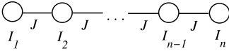
Figure 1: The system that we study in this paper is a linear chain of $n$ weakly interacting spins $1/2$ with Ising coupling between next neighbors. The coupling constant is the same for all pairs of connected spins.

Motivated by NMR spectroscopy of large molecules in solution, we assume that the relaxation rates of the longitudinal operators with components only in the $z$ direction, like $I_{iz}$, $2I_{iz}I_{(i+1)z}$ is negligible compared with relaxation rates for transverse operators like $I_{ix}$ , $2I_{iz}I_{(i+1)y}$ NMR . The transverse relaxation is modeled by the Lindbladian with the general form NMR

$$L(\rho)=\sum_{i}\pi a_{i}[I_{iz}[I_{iz},\rho]]+\sum_{i,j}\pi b_{ij}[2I_{iz}I_{jz}[2I_{iz}I_{jz},\rho]]\;.$$

In liquid state NMR spectroscopy, the two terms of the Lindblad operator model the relaxation mechanism caused by chemical shift anisotropy and dipole-dipole interaction respectively NMR . Here we neglect any interference effects between these two relaxation mechanisms Goldman1 . Relaxation rates $a_{i},b_{ij}$ depend on various physical parameters, such as the gyromagnetic ratios of the spins, the internuclear distance, the correlation time of molecular tumbling etc. We define the net transverse relaxation rate for spin $i$ as Khaneja1 $k_{a}^{i}=a_{i}+\sum_{j}b_{ij}$. Without loss of generality in the subsequent analysis, we assume that $k_{a}^{i}$ are equal and we denote this common transverse relaxation rate by $k$.

The time evolution (in the rotating frame) of the spin system density matrix $\rho$ is given by the master equation

$$\dot{\rho}=-i[H,\rho]+L(\rho)\;,$$ (2)

where $H=H_{c}+H_{rf}$ and $H_{rf}$ is the control Hamiltonian. In the NMR context, the available controls are the components of the transverse radio-frequency (RF) magnetic field. It is assumed that the resonance frequencies of the spins are well separated, so that each spin can be selectively excited (addressed) by an appropriate choice of the components of the RF field at its resonance frequency.

Consider now the problem of optimizing the polarization transfer

$$I_{1z}\rightarrow I_{nz}$$ (3)

along the linear spin chain shown in Fig. 1, in the presence of the relaxation mechanisms mentioned above. This problem can be stated as follows: Find the optimal transverse RF magnetic field in the control Hamiltonian $H_{rf}$ such that starting from $\rho(0)=I_{1z}$ and evolving under Eq. (2) the target expectation value $\langle I_{nz}\rangle=\mbox{tr}\{\rho(t)I_{nz}\}$ is maximized.

To fix ideas, we analyze the case when $n=3$

$$I_{1z}\rightarrow I_{3z}\;.$$ (4)

This transfer is achieved conventionally using INEPT like pulse sequences inept1 ; inept2 ; concat . Under the conventional transfer method, the initial state of the system $I_{1z}$ evolves through the following stages

$$I_{1z}\rightarrow 2I_{1z}I_{2z}\rightarrow 2I_{2z}I_{3z}\rightarrow I_{3z}.$$ (5)

In the first stage of the transfer, $I_{1z}\rightarrow 2I_{1z}I_{2z}$, spin $3$ is decoupled from the chain using standard decoupling methods Ernst and the initial polarization $I_{1z}$ on spin $1$ is rotated by RF field (an appropriate $\pi/2$ pulse) to coherence $I_{1x}$, which then evolves under coupling Hamiltonian $2I_{1z}I_{2z}$ to $2I_{1y}I_{2z}$. When the expectation value $\langle 2I_{1y}I_{2z}\rangle$ is maximized, another $\pi/2$ pulse is used to rotate $2I_{1y}I_{2z}$ to $2I_{1z}I_{2z}$. This is the INEPT pulse sequence. The next stage, $2I_{1z}I_{2z}\rightarrow 2I_{2z}I_{3z}$, is the so-called spin order transfer. Fig. 2 shows the population inversion corresponding to this transfer. By a suitable $\pi/2$ rotation of spin 2, the density operator $2I_{1z}I_{2z}$ is transformed to $2I_{1z}I_{2x}$, which then evolves to $2I_{2x}I_{3z}$. When the expectation value $\langle 2I_{2x}I_{3z}\rangle$ is maximized, another $\pi/2$ pulse is used to rotate $2I_{2x}I_{3z}$ to the spin order $2I_{2z}I_{3z}$. This is the Concatenated INEPT (CINEPT) pulse sequence. The final stage transfer, $2I_{2z}I_{3z}\rightarrow I_{3z}$, is similar to that in the first stage and is accomplished by the INEPT pulse sequence. The efficiency of these transfers is limited by the decay of transverse operators, due to the phenomenon of relaxation.

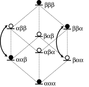
Figure 2: Energy level diagram for the spin order transfer $2I_{1z}I_{2z}\rightarrow 2I_{2z}I_{3z}$. The dark circles represent population excess. State $\alpha$ corresponds to spin up and state $\beta$ to spin down.

In our recent work on relaxation optimized control of coupled spin dynamics Khaneja1 , we showed that the efficiency of the first and the last step (the two INEPT stages) in Eq. (5) can be significantly improved by controlling precisely the way in which magnetization is transferred from longitudinal operators to transverse operators. In other words, instead of using $\pi/2$ (hard) pulses to rotate longitudinal to transverse operators (and the inverse), we can exploit the fact that longitudinal operators are long lived by making these rotations gradually, saving this way magnetization. This transfer strategy is called relaxation optimized pulse element (ROPE).

In this article we derive relaxation optimized pulse sequences for the intermediate transfer (the CINEPT stage),

$$2I_{1z}I_{2z}\rightarrow 2I_{2z}I_{3z}\;.$$ (6)

This relaxation optimized transfer of spin order can then be used as a building block for the polarization transfer (3) through the scheme

$$I_{1z}\rightarrow 2I_{1z}I_{2z}\rightarrow 2I_{2z}I_{3z}\rightarrow\ldots\rightarrow 2I_{(n-1)z}I_{nz}\rightarrow I_{nz}\;.$$ (7)

II The Optimal Control Problem and an Upper Bound for the Efficiency

In this section, we formulate the problem of transfer in Eq. (6) as a problem of optimal control and derive an upper bound on the transfer efficiency. To simplify notation, we introduce the following symbols for the expectation values of operators that play a part in the transfer. Let $z_{1}=\langle 2I_{1z}I_{2z}\rangle$, $x_{1}=\langle 2I_{1z}I_{2x}\rangle$, $y_{2}=\langle\sqrt{2}(2I_{1z}I_{2y}I_{3z}+I_{2y}/2)\rangle$, $x_{3}=-\langle 2I_{2x}I_{3z}\rangle$ and $z_{3}=\langle 2I_{2z}I_{3z}\rangle$. As a control variable we use the transverse RF magnetic field, pointing say in the $y$ direction (in the rotating frame), so $H_{rf}=\omega_{y}(t)I_{2y}$. Note that $\omega_{y}(t)$ is the component of the field in the rotating frame, so it is actually the envelope of the RF field. The carrier frequency of the RF field is the resonance frequency of spin 2. Using Eq. (2), we find that the evolution of the system, in time units of $1/(\pi J\sqrt{2})$, is given by

$$\left[\begin{array}[]{ccccc}\dot{z}_{1}\\ \dot{x}_{1}\\ \dot{y}_{2}\\ \dot{x}_{3}\\ \dot{z}_{3}\end{array}\right]=\left[\begin{array}[]{ccccc}0&-\Omega_{y}&0&0&0\\ \Omega_{y}&-\xi&-1&0&0\\ 0&1&-\xi&-1&0\\ 0&0&1&-\xi&-\Omega_{y}\\ 0&0&0&\Omega_{y}&0\\ \end{array}\right]\left[\begin{array}[]{ccccc}z_{1}\\ x_{1}\\ y_{2}\\ x_{3}\\ z_{3}\end{array}\right]\;,$$ (8)

where $\Omega_{y}(t)=\omega_{y}(t)/(\pi J\sqrt{2})$ and $\xi=k/(J\sqrt{2})$. The initial condition is $(z_{1},x_{1},y_{2},x_{3},z_{3})=(1,0,0,0,0)$.

The efficiency of the conventional method (CINEPT) for transfer $z_{1}\rightarrow z_{3}$, can be easily found. At $t=0$, $z_{1}$ is transferred to $x_{1}$ by application of a $(\pi/2)_{y}$ pulse on spin 2. Couplings evolve $x_{1}$ to $y_{2}$ which further evolves to $x_{3}$. As a function of time, $x_{3}(t)=e^{-\xi t}\sin^{2}(t/\sqrt{2})$. This is maximized for $t_{m}=\sqrt{2}\cot^{-1}(\xi/\sqrt{2})$. At $t=t_{m}$ a second $(\pi/2)_{y}$ pulse is applied on spin 2, rotating the maximum value from $x_{3}$ to $z_{3}$. This value is the efficiency $\eta_{CI}$ of the conventional method

$$\eta_{CI}=\exp(-\xi\sqrt{2}\cot^{-1}(\xi/\sqrt{2}))\sin^{2}(\cot^{-1}(\xi/\sqrt{2}))\;.$$ (9)

A better efficiency can be achieved if we store magnetization in the decoherence free longitudinal operators $z_{i}$ while the system is evolving. This is done by rotating $z_{i}$ to $x_{i}$ gradually, instead of using $\pi/2$ hard pulses. This is the physical concept behind the relaxation optimized transfer strategy. For the specific transfer examined in this article, we first find an upper bound for the maximum efficiency and in the next section we calculate numerically the magnetic field $\Omega_{y}(t)$ that approaches this bound.

In order to derive the upper bound, we use an augmented system instead of the original one (8). The augmentation is done in two steps. First, we suppose that we can rotate $z_{1}$ to $x_{1}$ and $x_{3}$ to $z_{3}$ independently using two different controls, say $\Omega_{1}(t)$ and $\Omega_{3}(t)$, instead of the common control $\Omega_{y}(t)$. Next, we provide $y_{2}$ with a relaxation free partner $z_{2}$ and with a control $\Omega_{2}(t)$ which can rotate $y_{2}$ to $z_{2}$. The augmented system is

$$\left[\begin{array}[]{cccccc}\dot{z}_{1}\\ \dot{z}_{2}\\ \dot{z}_{3}\\ \dot{x}_{1}\\ \dot{y}_{2}\\ \dot{x}_{3}\end{array}\right]=\left[\begin{array}[]{cccccc}0&0&0&-\Omega_{1}&0&0\\ 0&0&0&0&-\Omega_{2}&0\\ 0&0&0&0&0&-\Omega_{3}\\ \Omega_{1}&0&0&-\xi&-1&0\\ 0&\Omega_{2}&0&1&-\xi&-1\\ 0&0&\Omega_{3}&0&1&-\xi\end{array}\right]\left[\begin{array}[]{cccccc}z_{1}\\ z_{2}\\ z_{3}\\ x_{1}\\ y_{2}\\ x_{3}\end{array}\right]\;.$$ (10)

Observe that system (10) reduces to system (8) for $\Omega_{1}=-\Omega_{3}=\Omega_{y}$ and $\Omega_{2}=0$. Thus, if we know the maximum achievable value of $z_{3}$ starting from $(1,0,0,0,0,0)$ and evolving under system (10), then this is an upper bound for the maximum achievable value of $z_{3}$ with evolution described by the original system (8).

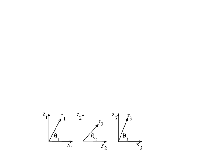
Figure 3: Auxiliary variables $r_{i}$.

Let $r_{1}=\sqrt{x_{1}^{2}+z_{1}^{2}}$, $r_{2}=\sqrt{y_{2}^{2}+z_{2}^{2}}$ and $r_{3}=\sqrt{x_{3}^{2}+z_{3}^{2}}$. Using $\Omega_{i}(t)$ we can control the angles $\theta_{i}$, shown in Fig. 3, independently. If we assume that the control can be done arbitrarily fast as compared to the evolution of couplings or relaxation rates then we can think of $\theta_{i}$ as control variables. The equations for the evolution of $r_{i}$ are

$$\left[\begin{array}[]{ccc}\dot{r}_{1}\\ \dot{r}_{2}\\ \dot{r}_{3}\end{array}\right]=\left[\begin{array}[]{ccc}-\xi u_{1}^{2}&-u_{1}u_{2}&0\\ u_{1}u_{2}&-\xi u_{2}^{2}&-u_{2}u_{3}\\ 0&u_{2}u_{3}&-\xi u_{3}^{2}\end{array}\right]\left[\begin{array}[]{ccc}r_{1}\\ r_{2}\\ r_{3}\end{array}\right],$$ (11)

where the new control parameters are $u_{i}(t)=\cos(\theta_{i}(t))$. The goal is to find the largest achievable value of $r_{3}$ starting from $(r_{1},r_{2},r_{3})=(1,0,0)$ by appropriate choice of $u_{i}(t)$. This problem can be solved analytically. The optimal solution is characterized by maintaining vanishingly small values of $dr_{2}/dt$, i.e., $(u_{1}r_{1}-u_{3}r_{3})/u_{2}r_{2}=\xi$ and by $u_{3}r_{3}/u_{1}r_{1}=\kappa$, where

$$\kappa=\frac{(\sqrt{\xi^{2}+2}-\xi)^{2}}{2}.$$ (12)

The maximum achievable value of $r_{3}$ is also $\kappa$. We prove it in the following.

Using variables $p_{i}={r_{i}^{2}}$, $m_{i}=u_{i}r_{i}/\sqrt{\sum_{i}^{3}(u_{i}r_{i})^{2}}$, and $d\tau/dt=\sum_{i}^{3}(u_{i}r_{i})^{2}$ , equation (11) can be re-written as

$$\frac{d}{d\tau}\left[\begin{array}[]{c}{p}_{1}(\tau)\\ {p}_{2}(\tau)\\ {p}_{3}(\tau)\end{array}\right]=\ diag(Am(\tau)m^{T}(\tau))\;,$$ (13)

where

$$A=2\left[\begin{array}[]{ccc}-\xi&-1&0\\ 1&-\xi&-1\\ 0&1&-\xi\end{array}\right],$$ (14)

$m^{T}=(m_{1},m_{2},m_{3})$ and $diag(X)$ represents the vector containing diagonal entries of the square matrix $X$. The goal is to find the controls $m_{i}(\tau)$ ($\sum_{i}m_{i}^{2}(\tau)=1$) and the largest achievable value of $p_{3}$ starting from $(p_{1},p_{2},p_{3})=(1,0,0)$. Eq. (13) implies that

$$\left[\begin{array}[]{c}{p}_{1}(T)\\ {p}_{2}(T)\\ {p}_{3}(T)\end{array}\right]=\left[\begin{array}[]{c}{p}_{1}(0)\\ {p}_{2}(0)\\ {p}_{3}(0)\end{array}\right]+diag(A\int_{0}^{T}m(\tau)m^{T}(\tau)d\tau)\;.$$

Let $M=\int_{0}^{T}m(\tau)m^{T}(\tau)d\tau$. Note that $M$ is a symmetric, positive semidefinite matrix. By definition $p_{i}(\tau)\geq 0$ for all $\tau$. At final time $T$, we must have $p_{1}(T)=0$ and $p_{2}(T)=0$, as any nonzero value of $p_{1}(T)$ or $p_{2}(T)$ can be partly transferred to $p_{3}$ and the final value of $p_{3}(T)$ further increased. Since $(p_{1}(0),p_{2}(0),p_{3}(0))=(1,0,0)$, it implies that $M$ should be such that $(AM)_{11}=-1$, $(AM)_{22}=0$ and $(AM)_{33}$ is maximized over all positive semidefinite $M$ satisfying the above constraints. This problem is a special case of a semidefinite programming problem Boyd . If the symmetric part of matrix $A$ is negative definite, as in our case (14), then it can be shown that the optimal solution $M$ to the above stated semi-definite programming problem is a rank one matrix dionisis , i.e., $M=mm^{T}$ for some constant $m$ and therefore the ratio $u_{i}r_{i}/u_{j}r_{j}$ in (11) is constant throughout. The condition $(AM)_{22}=0$, implies $(u_{1}r_{1}-u_{3}r_{3})/\xi=u_{2}r_{2}$. Substituting for $u_{2}r_{2}$ in (11), we obtain

$$\left[\begin{array}[]{cc}\dot{r}_{1}\\ \dot{r}_{3}\end{array}\right]=\left[\begin{array}[]{cc}-(\xi+1/\xi)u_{1}^{2}&u_{1}u_{3}/\xi\\ u_{1}u_{3}/\xi&-(\xi+1/\xi)u_{3}^{2}\end{array}\right]\left[\begin{array}[]{ccc}r_{1}\\ r_{3}\end{array}\right],$$ (15)

We now simply need to maximize the gain in $r_{3}$ to loss in $r_{1}$, i.e., the ratio $\dot{r}_{3}/(-\dot{r}_{1})$. This yields $u_{3}r_{3}/u_{1}r_{1}=\kappa$, with $\kappa$ given in (12). The corresponding maximum efficiency for transfer $r_{1}\rightarrow r_{3}$ is also $\kappa$. This is the maximum efficiency for transfer $z_{1}\rightarrow z_{3}$ under the augmented system (10), and thus an upper bound for the efficiency of the same transfer under the original system (8).

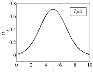
(a)	(b)
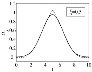
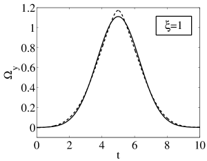
(c)	(d)
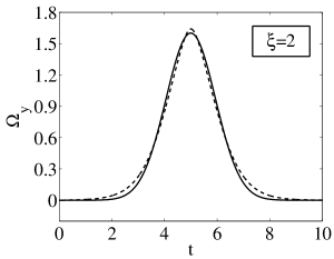
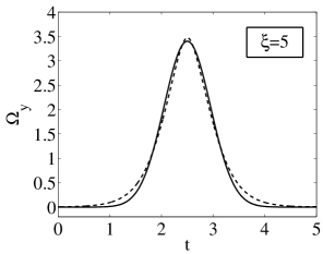
(e)	(f)

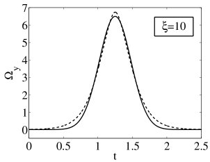
Figure 4: Optimal pulse (dashed line) calculated using a numerical optimization method based on a steepest descent algorithm, for various values of the normalized relaxation parameter $\xi$. The Gaussian pulse (solid line) approximates very well the optimal pulse shape and gives a similar efficiency. This suggests that instead of using the initial numerical optimization method, we can use Gaussian pulses of the form (16), optimized with respect to $A$ and $\sigma$ for each value of $\xi$.

III Numerical Calculation of the Optimal RF field and Discussion

Having established an analytical upper bound (12) for the efficiency, we now try to find numerically a RF field $\Omega_{y}(t)$ that approaches this bound, for each value of the parameter $\xi$. We emphasize that in this section the original system (8) is employed.

At first, we use a numerical optimization method based on a steepest descent algorithm. For the application of the method we use a finite time window $T$. For values of normalized relaxation $\xi$ in $(0-1)$, a time interval $T=10$ (normalized time units) is enough. For larger values of $\xi$ we can use even shorter $T$. The optimal RF field $\Omega_{y}(t)$ that we find with this method, for various $\xi$, is shown in Fig. 4. Note that as $\xi$ increases, the optimal pulse becomes shorter in time and acquires a larger peak value. The reason for this is that for larger $\xi$ the transfer $z_{1}\rightarrow z_{3}$ should be done faster, in order to reduce the time spent in the transverse plane and hence the relaxation losses. Now observe that the optimal pulse shape can be very well approximated by a Gaussian profile of the form

$$\Omega_{y}(t)=A\exp{\left[\left(\frac{t-T/2}{\sqrt{2}\sigma}\right)^{2}\right]}\;,$$ (16)

with $A,\sigma$ appropriately chosen. As a result, the efficiency that we find using the appropriate Gaussian pulse is very close to that we find using the original pulse. This suggests that instead of using the initial numerical optimization method, we can use Gaussian pulses of the form (16), optimized with respect to $A$ and $\sigma$ for each value of $\xi$. The optimal $A,\sigma$ are found by numerical simulations. For each $\xi$ we simulate the equations of system (8) with $\Omega_{y}(t)$ given by Eq. (16), for many values of $A$ and $\sigma$. We choose those values that give the maximum $z_{3}(T)$. In table I, we show the optimal $A,\sigma$ for various values $\xi\in[0,1]$. We also show the corresponding efficiency, as well as the efficiency achieved by the initial numerical optimization method. Observe how close lie these two groups of values. The choice of the Gaussian shape is indeed successful.

Table 1: For various values of $\xi\in[0,1]$, the optimal values of $A,\sigma$ and the corresponding efficiency are shown. We present also for comparison the efficiency achieved by the steepest descent method.

$\xi$	$A$	$\sigma$	Gaussian Pulse	Steepest Descent
1.00	1.11	1.30	0.2510	0.2512
0.95	1.09	1.32	0.2661	0.2662
0.90	1.07	1.34	0.2824	0.2825
0.85	1.05	1.36	0.3000	0.3001
0.80	1.03	1.38	0.3190	0.3191
0.75	1.02	1.39	0.3396	0.3397
0.70	1.00	1.41	0.3619	0.3620
0.65	0.98	1.43	0.3861	0.3863
0.60	0.97	1.44	0.4124	0.4126
0.55	0.96	1.44	0.4410	0.4413
0.50	0.95	1.44	0.4721	0.4726
0.45	0.94	1.45	0.5060	0.5067
0.40	0.93	1.46	0.5428	0.5439
0.35	0.92	1.46	0.5830	0.5846
0.30	0.91	1.46	0.6270	0.6292
0.25	0.90	1.47	0.6750	0.6780
0.20	0.89	1.48	0.7277	0.7315
0.15	0.88	1.48	0.7855	0.7900
0.10	0.85	1.52	0.8494	0.8536
0.05	0.79	1.60	0.9203	0.9232
0.00	0.73	1.71	0.9999	1.0000

Fig. 5 shows the efficiency of the conventional method (CINEPT), i.e., $\eta_{CI}$ from Eq. (9), the efficiency of our method (SPORTS ROPE, SPin ORder TranSfer with Relaxation Optimized Pulse Element), and the upper bound $\kappa$ from Eq. (12), for the values of relaxation parameter $\xi$ shown in table I. Note that for large $\xi$ (large relaxation rates), SPORTS ROPE gives a significant improvement over CINEPT. Also note that it approaches fairly well the upper bound.

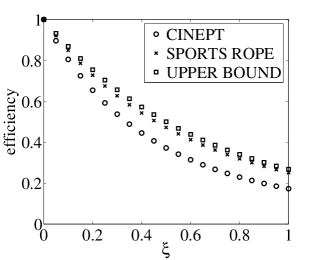
Figure 5: Efficiency for the conventional method (CINEPT), Eq. (9), and for our method (SPORTS ROPE), for the values of $\xi$ shown in table I. The upper bound (12) for the efficiency is also shown.

Using the Gaussian pulse shape we can get a quantitative impression of the robustness of SPORTS ROPE. In Fig. 6 we give a gray-scale topographic plot of the efficiency ($z_{3}(T)$ with $T=10$) as a function of $A$ and $\sigma$ for $\xi=1$. The maximum value can be found from table I and is 0.2510. The white region corresponds to values $\geq 0.24$, while the black region to values $<\eta_{CI}(\xi=1)=0.1727$. The intermediate gray regions correspond to values between these two limits. Obviously, SPORTS ROPE is quite robust.

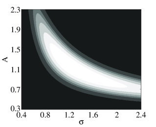
Figure 6: Gray-scale topographic plot of the efficiency as a function of the amplitude $A$ and the standard deviation $\sigma$ of the Gaussian pulse for $\xi=1$. The maximum value can be found from table I and is 0.2510. The white region corresponds to values $\geq 0.24$, while the black region to values $<\eta_{CI}$($\xi$=1) = 0.1727. The intermediate gray regions correspond to the intervals $[0.23,0.24),[0.22,0.23),[0.21,0.22),[0.20,0.21),[0.1727,0.20)$ (from white to black).

In Fig. 7(a), we plot the time evolution of the various transfer functions (expectation values of operators) that participate in the transfer $z_{1}\rightarrow z_{3}$, when the optimal Gaussian pulse for $\xi=1$, shown in Fig. 4(c), is applied to system (8). Observe the gradual building of the intermediate variables $x_{1},y_{2}$ and $x_{3}$. Note that $dr_{2}/dt=\dot{y}_{2}\neq 0$. There is no contradiction with the optimality condition $dr_{2}/dt=0$ derived in section II during the calculation of the upper bound, since this condition refers to the augmented system (10) and not the original one (8) used here. In Fig. 7(b) we plot the angle $\theta_{3}=\tan^{-1}{(z_{3}/x_{3})}$ of the vector $\textit{{r}}_{3}$ with the $x$ axis, as a function of time. Observe that initially $\textit{{r}}_{3}$ is parallel to $x$ axis ($\theta_{3}=0$), but under the action of the Gaussian pulse is rotated gradually to $z$ axis ($\theta_{3}=\pi/2$). This gradual rotation of $\textit{{r}}_{3}$ (as well as of $\textit{{r}}_{1}$) is a characteristic feature of the SPORTS ROPE transfer scheme.

(a)

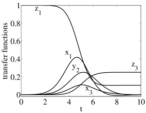
(b)

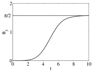
Figure 7: (a) Time evolution of the various transfer functions (expectation values of operators) participating in the transfer $z_{1}\rightarrow z_{3}$, when the optimal Gaussian pulse for $\xi=1$, shown in Fig. 4(c), is applied to system (8). (b) The angle $\theta_{3}=\tan^{-1}{(z_{3}/x_{3})}$ of the vector $\textit{{r}}_{3}$ with the $x$ axis, as a function of time. Observe that initially $\textit{{r}}_{3}$ is parallel to $x$ axis ($\theta_{3}=0$), but under the action of the Gaussian pulse is rotated gradually to $z$ axis ($\theta_{3}=\pi/2$).

We remark that for the general transfer $I_{1z}\rightarrow I_{nz}$, more than one intermediate steps $2I_{(i-1)z}I_{iz}\rightarrow 2I_{iz}I_{(i+1)z}$ are necessary. Since the equations that describe the $i^{th}$ transfer are the same as $(\ref{eq:path})$, we just need to apply the same Gaussian pulse but centered, in the frequency domain, at the resonance frequency of spin $i$. In this sequence of Gaussian pulses we should add at the beginning and at the end the optimal pulses for the first and the final step, respectively, see Eq. (7). These pulses can be calculated using the theory presented in Khaneja1 . Finally, note that the same scheme can be used for the coherence transfer $I_{1\alpha}\rightarrow I_{n\beta}$, where $\alpha,\beta$ can be $x$ or $y$. We just need to add the initial and final $\pi/2$ pulses that accomplish the rotations $I_{1\alpha}\rightarrow I_{1z}$, $I_{nz}\rightarrow I_{n\beta}$.

IV Conclusion

In this paper, we derived an upper bound on the efficiency of spin order transfer along an Ising spin chain, in the presence of relaxation, and calculated numerically relaxation optimized pulse sequences approaching this bound. Using these methods, a significant reduction in relaxation losses is achieved, compared to standard techniques, when transverse relaxation rates are much larger than the longitudinal relaxation rates and comparable to couplings between spins. These relaxation optimized methods can be used as a building block for transfer of polarization or coherence between distant spins on a spin chain. This problem is ubiquitous in multi-dimensional NMR spectroscopy and is also interesting in the context of quantum information processing.

- (1) N. Khaneja, T. Reiss, B. Luy, and S.J. Glaser, J. Magn. Reson. 162, 311 (2003).
- (2) N. Khaneja, B. Luy, and S.J. Glaser (2003) Proc. Natl. Acad. Sci. U.S.A 100, 13162 (2003).
- (3) D. Stefanatos, N. Khaneja, and S.J. Glaser, Phys. Rev. A, 69, 022319 (2004).
- (4) N. Khaneja, Jr. Shin Li, C. Kehlet, B. Luy, S.J. Glaser, Proc. Natl. Acad. Sci. USA. 101, 14742-47 (2004).
- (5) B.E. Kane, Nature 393, 133 (1998).
- (6) F. Yamaguchi, Y. Yamamoto, Appl. Phys. A 68 (1999).
- (7) J. Cavanagh, W.J. Fairbrother, A.G. Palmer III, and N.J. Skelton, Protein NMR Spectroscopy (Academic Press, New York, 1996).
- (8) M. Goldman, Interference effects in the relaxation of a pair of unlike spin-1/2 nuclei, J. Magn. Reson. 60, 437 (1984).
- (9) G. A. Morris, R. Freeman, J. Am. Chem. Soc. 101, 760 (1979).
- (10) D. P. Burum, R. R. Ernst, J. Magn. Reson. 39, 163 (1980).
- (11) A. Majumdar, E. P. Zuiderweg, J. Magn. Reson. A 113, 19-31 (1995).
- (12) R.R. Ernst, G. Bodenhausen, A. Wokaun, Principles of Nuclear Magnetic Resonance in One and Two Dimensions, Clarendon Press, Oxford, 1987.
- (13) L. Vandenberghe, S. Boyd, SIAM Review 38, 49-95 (1996).
- (14) D. Stefanatos and N. Khaneja, math.OC/0504308, (2005).