\authorinfo

http://www.ipme.ru/zeitlin.html, http://www.ipme.nw.ru/zeitlin.html, E-mail: zeitlin@math.ipme.ru, anton@math.ipme.ru

IN QUANTUM PHYSICS.

II. WAVELETONS IN QUANTUM ENSEMBLES

Antonina N. Fedorova, Michael G. Zeitlin

IPME RAS, St. Petersburg, V.O. Bolshoj pr., 61, 199178, Russia

e-mail: zeitlin@math.ipme.ru

e-mail: anton@math.ipme.ru

http://www.ipme.ru/zeitlin.html

http://www.ipme.nw.ru/zeitlin.html

Localization and Pattern Formation in Quantum Physics.
II. Waveletons in Quantum Ensembles

Antonina N. Fedorova and Michael G. Zeitlin \skiplinehalf\supit IPME RAS St. Petersburg V.O. Bolshoj pr 61 199178 Russia

Abstract

In this second part we present a set of methods, analytical and numerical, which can describe behaviour in (non) equilibrium ensembles, both classical and quantum, especially in the complex systems, where the standard approaches cannot be applied. The key points demonstrating advantages of this approach are: (i) effects of localization of possible quantum states; (ii) effects of non-perturbative multiscales which cannot be calculated by means of perturbation approaches; (iii) effects of formation of complex/collective quantum patterns from localized modes and classification and possible control of the full zoo of quantum states, including (meta) stable localized patterns (waveletons). We demonstrate the appearance of nontrivial localized (meta) stable states/patterns in a number of collective models covered by the (quantum)/(master) hierarchy of Wigner-von Neumann-Moyal-Lindblad equations, which are the result of “wignerization” procedure (Weyl-Wigner-Moyal quantization) of classical BBGKY kinetic hierarchy, and present the explicit constructions for exact analytical/numerical computations. Our fast and efficient approach is based on variational and multiresolution representations in the bases of polynomial tensor algebras of generalized localized states (fast convergent variational-wavelet representation). We construct the representations for hierarchy/algebra of observables(symbols)/distribution functions via the complete multiscale decompositions, which allow to consider the polynomial and rational type of nonlinearities. The solutions are represented via the exact decomposition in nonlinear high-localized eigenmodes, which correspond to the full multiresolution expansion in all underlying hidden time/space or phase space scales. In contrast with different approaches we do not use perturbation technique or linearization procedures. Numerical modeling shows the creation of different internal structures from localized modes, which are related to the localized (meta) stable patterns (waveletons), entangled ensembles (with subsequent decoherence) and/or chaotic-like type of behaviour.

Abstract

keywords:

localization, pattern formation, multiscales, multiresolution, waveletons, (non) equilibrium ensembles

Optics & Photonics, SP200, San Diego, CA, July-August, 2005

1 INTRODUCTION: CLASSICAL AND QUANTUM ENSEMBLES

In this paper we consider the applications of a numerical-analytical technique based on local nonlinear harmonic analysis to the description of quantum ensembles. The corresponding class of individual Hamiltonians has the form

\displaystyle\hat{H}(\hat{p},\hat{q})=\frac{\hat{p}^{2}}{2m}+U(\hat{p},\hat{q}),

(1)

where $U(\hat{p},\hat{q})$ is an arbitrary polynomial function on $\hat{p}$ , $\hat{q}$ , and plays the key role in many areas of physics [1]. Many cases, related to some physics models, are considered in [2]-[8]. It is a continuation of our more qualitative approach considered in part I [9]. In this part our goals are some attempt of classification and the constructions of explicit numerical-analytical representations for the existing quantum states in the class of models described (non) equilibrium ensembles and related collective models. There is a hope on the understanding of relation between the structure of initial Hamiltonians and the possible types of quantum states and the qualitative type of their behaviour. Inside the full spectrum there are at least three possibilities which are the most important from our point of view: localized states, chaotic-like or/and entangled patterns, localized (stable) patterns (qualitative definitions/descriptions can be found in part I [9]). All such states are interesting in the different areas of physics [1]. Our starting point is the general point of view of a deformation quantization approach at least on the naive Moyal/Weyl/Wigner level. The main point of such approach is based on ideas from [1], which allow to consider the algebras of quantum observables as the deformations of commutative algebras of classical observables (functions). So, if we have the classical counterpart of Hamiltonian (1) as a model for classical dynamics and the Poisson manifold $M$ (or symplectic manifold or Lie coalgebra, etc) as the corresponding phase space, then for quantum calculations we need first of all to find an associative (but non-commutative) star product $*$ on the space of formal power series in $\hbar$ with coefficients in the space of smooth functions on $M$ such that

\displaystyle f*g=fg+\hbar\{f,g\}+\sum_{n\geq 2}\hbar^{n}B_{n}(f,g),

(2)

where $\{f,g\}$ is the Poisson brackets, $B_{n}$ are bidifferential operators. In the naive calculations we may use the simple formal rule:

\displaystyle*

\displaystyle\equiv

\displaystyle\exp\Big{(}\frac{i\hbar}{2}(\overleftarrow{\partial}_{q}\overrightarrow{\partial}_{p}-\overleftarrow{\partial}_{p}\overrightarrow{\partial}_{q})\Big{)}

(3)

In this paper we consider the calculations of the Wigner functions $W(p,q,t)$ (WF) corresponding to the classical polynomial Hamiltonian $H(p,q,t)$ as the solution of the Wigner-von Neumann equation [1]:

\displaystyle i\hbar\frac{\partial}{\partial t}W=H*W-W*H

(4)

and related Wigner-like equations for different ensembles. According to the Weyl transform, a quantum state (wave function or density operator $\rho$ ) corresponds to the Wigner function, which is the analogue in some sense of classical phase-space distribution [1]. We consider the following operator form of differential equations for time-dependent WF, $W=W(p,q,t)$ :

\displaystyle W_{t}=\frac{2}{\hbar}\sin\Big{[}\frac{\hbar}{2}(\partial^{H}_{q}\partial^{W}_{p}-\partial^{H}_{p}\partial^{W}_{q})\Big{]}\cdot HW

(5)

which is a result of the Weyl transform or “wignerization” of von Neumann equation for density matrix:

i\hbar\frac{\partial\rho}{\partial t}=[H,\rho]

(6)

1.1 BBGKY Ensembles

We start from set-up for kinetic BBGKY hierarchy (as c-counterpart of proper q-hierarchy). We present the explicit analytical construction for solutions of both hierarchies of equations, which is based on tensor algebra extensions of multiresolution representation and variational formulation. We give explicit representation for hierarchy of n-particle reduced distribution functions in the base of high-localized generalized coherent (regarding underlying generic symmetry (affine group in the simplest case)) states given by polynomial tensor algebra of our basis functions (wavelet families), which takes into account contributions from all underlying hidden multiscales from the coarsest scale of resolution to the finest one to provide full information about stochastic dynamical process. The difference between classical and quantum case is concetrated in the structure of the set of operators included in the set-up and, surely, depends on the method of quantization. But, in the naive Wigner-Weyl approach for quantum case the symbols of operators play the same role as usual functions in classical case. In some sense, our approach resembles Bogolyubov’s one and related approaches but we don’t use any perturbation technique (like virial expansion) or linearization procedures. Most important, that numerical modeling in both cases shows the creation of different internal (coherent) structures from localized modes, which are related to stable (equilibrium) or unstable type of behaviour and corresponding pattern (waveletons) formation.

Let M be the phase space of ensemble of N particles ( ${\rm dim}M=6N$ ) with coordinates

\displaystyle x_{i}=(q_{i},p_{i}),\quad i=1,...,N,\qquad q_{i}=(q^{1}_{i},q^{2}_{i},q^{3}_{i})\in R^{3},\qquad p_{i}=(p^{1}_{i},p^{2}_{i},p^{3}_{i})\in R^{3},\qquad q=(q_{1},\dots,q_{N})\in R^{3N}.

(7)

Individual and collective measures are:

\displaystyle\mu_{i}=\mathrm{d}x_{i}=\mathrm{d}q_{i}\mathrm{d}p_{i},\quad\mu=\prod^{N}_{i=1}\mu_{i}

(8)

Distribution function $D_{N}(x_{1},\dots,x_{N};t)$ satisfies Liouville equation of motion for ensemble with Hamiltonian $H_{N}$ and normalization constraint:

\displaystyle\frac{\partial D_{N}}{\partial t}=\{H_{N},D_{N}\},\qquad\int D_{N}(x_{1},\dots,x_{N};t)\mathrm{d}\mu=1

(9)

where Poisson brackets are:

\displaystyle\{H_{N},D_{N}\}=\sum^{N}_{i=1}\Big{(}\frac{\partial H_{N}}{\partial q_{i}}\frac{\partial D_{N}}{\partial p_{i}}-\frac{\partial H_{N}}{\partial p_{i}}\frac{\partial D_{N}}{\partial q_{i}}\Big{)}

(10)

Our constructions can be applied to the following general Hamiltonians:

\displaystyle H_{N}=\sum^{N}_{i=1}\Big{(}\frac{p^{2}_{i}}{2m}+U_{i}(q)\Big{)}+\sum_{1\leq i\leq j\leq N}U_{ij}(q_{i},q_{j})

(11)

where potentials $U_{i}(q)=U_{i}(q_{1},\dots,q_{N})$ and $U_{ij}(q_{i},q_{j})$ are not more than rational functions on coordinates. Let $L_{s}$ and $L_{ij}$ be the Liouvillean operators (vector fields)

\displaystyle L_{s}=\sum^{s}_{j=1}\Big{(}\frac{p_{j}}{m}\frac{\partial}{\partial q_{j}}-\frac{\partial u_{j}}{\partial q}\frac{\partial}{\partial p_{j}}\Big{)}-\sum_{1\leq i\leq j\leq s}L_{ij},\qquad L_{ij}=\frac{\partial U_{ij}}{\partial q_{i}}\frac{\partial}{\partial p_{i}}+\frac{\partial U_{ij}}{\partial q_{j}}\frac{\partial}{\partial p_{j}}

(12)

For s=N we have the following representation for Liouvillean vector field $L_{N}=\{H_{N},\cdot\}$ and the corresponding ensemble equation of motion:

\displaystyle\frac{\partial D_{N}}{\partial t}+L_{N}D_{N}=0

(13)

$L_{N}$ is self-adjoint operator regarding standard pairing on the set of phase space functions. Let

\displaystyle F_{N}(x_{1},\dots,x_{N};t)=\sum_{S_{N}}D_{N}(x_{1},\dots,x_{N};t)

(14)

be the N-particle distribution function ( $S_{N}$ is permutation group of N element s). Then we have the hierarchy of reduced distribution functions ( $V^{s}$ is the corresponding normalized volume factor)

\displaystyle F_{s}(x_{1},\dots,x_{s};t)=V^{s}\int D_{N}(x_{1},\dots,x_{N};t)\prod_{s+1\leq i\leq N}\mu_{i}

(15)

After standard manipulations we arrived to c-BBGKY hierarchy:

\displaystyle\frac{\partial F_{s}}{\partial t}+L_{s}F_{s}=\frac{1}{\upsilon}\int\mathrm{d}\mu_{s+1}\sum^{s}_{i=1}L_{i,s+1}F_{s+1}

(16)

It should be noted that we may apply our approach even to more general formulation. As in the general as in particular situations (cut-off, e.g.) we are interested in the cases when

\displaystyle F_{k}(x_{1},\dots,x_{k};t)=\prod^{k}_{i=1}F_{1}(x_{i};t)+G_{k}(x_{1},\dots,x_{k};t),

(17)

where $G_{k}$ are correlators, really have additional reductions as in the simplest case of one-particle truncation (Vlasov/Boltzmann-like systems). So, the proper dynamical formulation is reduced to the (infinite) set of equations for correlators/partition functions. Then by using physical motivated reductions or/and during the corresponding cut-off procedure we obtain, instead of linear and pseudodifferential (in general case) equations, their finite-dimensional but nonlinear approximations with the polynomial type of nonlinearities (more exactly, multilinearities). Our key point in the following consideration is the proper generalization of naive perturbative multiscale Bogolyubov’s structure restricted by the set of additional physical hypotheses.

1.2 Quantum ensembles

Let us start from the second quantized representation for an algebra of observables

A=(A_{0},A_{1},\dots,A_{s},...)

(18)

in the standard form

\displaystyle A=A_{0}+\int dx_{1}\Psi^{+}(x_{1})A_{1}\Psi(x_{1})+\dots+(s!)^{-1}\int dx_{1}\dots dx_{s}\Psi^{+}(x_{1})\dots\Psi^{+}(x_{s})A_{s}\Psi(x_{s})\dots\Psi(x_{1})+\dots

(19)

N-particle Wigner functions

	$\displaystyle W_{s}(x_{1},\dots,x_{s})$	$\displaystyle=$	$\displaystyle\int dk_{1}\dots dk_{s}{\rm exp}\big{(}-i\sum^{s}_{i=1}k_{i}p_{i}\big{)}{\rm Tr}\rho\Psi^{+}\big{(}q_{1}-\frac{1}{2}\hbar k_{1}\big{)}\dots$
			$\displaystyle\Psi^{+}\big{(}q_{s}-\frac{1}{2}\hbar k_{s}\big{)}\Psi\big{(}q_{s}+\frac{1}{2}\hbar k_{s}\big{)}\dots\Psi\big{(}q_{1}+\frac{1}{2}\hbar k_{s}\big{)}$

allow us to consider them as some quasiprobabilities and provide useful bridge between c- and q-cases:

<A>={\rm Tr}\rho A=\sum^{\infty}_{s=0}(s!)^{-1}\int\prod_{i=1}^{s}d\mu_{i}A_{s}(x_{1},\dots,x_{s})W_{s}(x_{1},\dots,x_{s})

(21)

The full description for quantum ensemble can be done by the whole hierarchy of functions (symbols):

W=\{W_{s}(x_{1},\dots,x_{s}),s=0,1,2\dots\}

(22)

So, we may consider the following q-hierarchy as the result of “wignerization” procedure for c-BBGKY one:

	$\displaystyle\partial_{t}W_{s}(t,x_{1},\dots,x_{s})$	$\displaystyle=$	$\displaystyle\sum^{s}_{j=1}L_{j}^{0}W_{s}(x_{1},\dots,x_{s})+\sum_{j<n}\sum^{s}_{n=1}L_{j,n}W_{s}(x_{1},\dots,x_{s})$
		$\displaystyle+$	$\displaystyle\sum^{s}_{j=1}\int dx_{s+1}\delta(k_{s+1})L_{j,s+1}W_{s+1}(x_{1},\dots,x_{s+1})$

where

L^{0}_{j}=-\big{(}\frac{i}{m}\big{)}k_{j}p_{j}

(24)

\displaystyle L_{j,n}=(i\hbar)^{-1}\int d\ell\tilde{V_{l}}\Bigg{[}{\rm exp}\Bigg{(}-\frac{1}{2}\hbar\ell\big{(}\frac{\partial}{\partial p_{j}}-\frac{\partial}{\partial p_{n}}\big{)}\Bigg{)}-{\rm exp}\bigg{(}\frac{1}{2}\hbar\ell\big{(}\frac{\partial}{\partial p_{j}}-\frac{\partial}{\partial p_{n}}\big{)}\Bigg{)}\Bigg{]}{\rm exp}\Bigg{(}-\ell\big{(}\frac{\partial}{\partial k_{j}}-\frac{\partial}{\partial k_{n}}\big{)}\Bigg{)}

(25)

In quantum statistics the ensemble properties are described by the density operator

\rho(t)=\sum_{i}w_{i}|\Psi_{i}(t)><\Psi_{i}(t)|,\quad\sum_{i}w_{i}=1

(26)

After Weyl transform we have the following decomposition via partial Wigner functions $W_{i}(p,q,t)$ for the whole ensemble Wigner function:

W(p,q,t)=\sum_{i}w_{i}W_{i}(p,q,t)

(27)

where the partial Wigner functions

\displaystyle W_{n}(q,p,t)\equiv\frac{1}{2\pi\hbar}\int\mathrm{d}\xi{\rm exp}\Big{(}-\frac{i}{\hbar}p\xi\Big{)}\Psi^{*}_{n}(q-\frac{1}{2}\xi,t)\Psi_{n}(q+\frac{1}{2}\xi,t)

(28)

are solutions of proper Wigner equations:

\displaystyle\frac{\partial W_{n}}{\partial t}=-\frac{p}{m}\frac{\partial W_{n}}{\partial q}+\sum^{\infty}_{\ell=0}\frac{(-1)^{\ell}(\hbar/2)^{2\ell}}{(2\ell+1)!}\frac{\partial^{2\ell+1}U_{n}(q)}{\partial q^{2\ell+1}}\frac{\partial^{2\ell+1}W_{n}}{\partial p^{2\ell+1}}

(29)

Our approach, presented below, in some sense has allusion on the analysis of the following standard simple model considered in [1]. Let us consider model of interaction of nonresonant atom with quantized electromagnetic field:

\displaystyle\hat{H}=\frac{\hat{p}_{x}^{2}}{2m}+U(\hat{x}),\qquad U(\hat{x})=U_{0}(z,t)g(\hat{x})\hat{a}^{+}\hat{a}

(30)

where potential $U$ depends on creation/annihilation operators and some polynomial on $\hat{x}$ operator function (or approximation) $g(\hat{x})$ . It is possible to solve Schroedinger equation

\displaystyle i\hbar\frac{\mathrm{d}|\Psi>}{\mathrm{d}t}=\hat{H}|\Psi>

(31)

by the simple ansatz

\displaystyle|\Psi(t)>=\sum_{-\infty}^{\infty}w_{n}\int\mathrm{d}x\Psi_{n}(x,t)|x>\otimes|n>

(32)

which leads to the hierarchy of analogous equations with potentials created by n-particle Fock subspaces

\displaystyle i\hbar\frac{\partial\Psi_{n}(x,t)}{\partial t}=\Big{\{}\frac{\hat{p}_{x}^{2}}{2m}+U_{0}(t)g(x)n\Big{\}}\Psi_{n}(x,t)

(33)

where $\Psi_{n}(x,t)$ is the probability amplitude of finding the atom at the time $t$ at the position $x$ and the field in the $n$ Fock state. Instead of this, we may apply the Wigner approach starting with proper full density matrix

	$\displaystyle\hat{\rho}=\|\Psi(t)><\Psi(t)\|=$		(34)
	$\displaystyle\sum_{n^{\prime},n^{\prime\prime}}w_{n^{\prime}}w^{}_{n^{\prime\prime}}\int\mathrm{d}x^{\prime}\int\mathrm{d}x^{\prime\prime}\Psi_{n^{\prime}}(x^{\prime},t)\Psi^{}_{n^{\prime\prime}}(x^{\prime\prime},t)\|x^{\prime}><x^{\prime\prime}\|\otimes\|n^{\prime}><n^{\prime\prime}\|$

Standard reduction gives pure atomic density matrix

	$\displaystyle\hat{\rho}_{a}\equiv\int^{\infty}_{n=0}<n\|\hat{\rho}\|n>=$		(35)
	$\displaystyle\sum\|w_{n}\|^{2}\int\mathrm{d}x^{\prime}\int\mathrm{d}x^{\prime\prime}\Psi_{n}(x^{\prime},t)\Psi^{*}_{n}(x^{\prime\prime},t)\|x^{\prime}><x^{\prime\prime}\|$

Then we have incoherent superposition

W(x,p,t)=\sum^{\infty}_{n=0}|w_{n}|^{2}W_{n}(x,p,t)

(36)

of the atomic Wigner functions (28) corresponding to the atom motion in the potential $U_{n}(x)$ (which is not more than polynomial in $x$ ) generated by $n$ -level Fock state. They are solutions of proper Wigner equations (29).

The next case describes the important decoherence process. Let us have collective and environment subsystems with their own Hilbert spaces

\mathcal{H}=\mathcal{H}_{c}\otimes\mathcal{H}_{e}

(37)

Relevant dynamics is described by three parts including interaction

H=H_{c}\otimes I_{e}+I_{c}\otimes H_{e}+H_{int}

(38)

For analysis, we can choose Lindblad master equation [1]

\displaystyle\dot{\rho}=\frac{1}{i\hbar}[H,\rho]-\sum_{n}\gamma_{n}(L^{+}_{n}L_{n}\rho+\rho L^{+}_{n}L_{n}-2L_{n}\rho L^{+}_{n})

(39)

which preserves the positivity of density matrix and it is Markovian but it is not general form of exact master equation. Other choice is Wigner transform of master equation and it is more preferable for us

\displaystyle\dot{W}=\{H,W\}_{PB}+\sum_{n\geq 1}\frac{\hbar^{2n}(-1)^{n}}{2^{2n}(2n+1)!}\partial^{2n+1}_{q}U(q)\partial_{p}^{2n+1}W(q,p)+2\gamma\partial_{p}pW+D\partial^{2}_{p}W

(40)

In the next section we consider the variational-wavelet approach for the solution of all these Wigner-like equations (4), (5), (6), (23), (29), (40) for the case of an arbitrary polynomial $U(q,p)$ , which corresponds to a finite number of terms in the series expansion in (5), (29), (40) or to proper finite order of $\hbar$ . Analogous approach can be applied to classical counterpart (16) also. Our approach is based on the extension of our variational-wavelet approach [2]-[8]. Wavelet analysis is some set of mathematical methods, which gives the possibility to take into account high-localized states, control convergence of any type of expansions and gives maximum sparse forms for the general type of operators in such localized bases. These bases are the natural generalization of standard coherent, squeezed, thermal squeezed states [1], which correspond to quadratical systems (pure linear dynamics) with Gaussian Wigner functions. The representations of underlying symmetry group (affine group in the simplest case) on the proper functional space of states generate the exact multiscale expansions which allow to control contributions to the final result from each scale of resolution from the whole underlying infinite scale of spaces. Numerical calculations according to methods of part I [9] explicitly demonstrate the quantum interference of generalized localized states, pattern formation from localized eigenmodes and the appearance of (stable) localized patterns (waveletons).

2 VARIATIONAL MULTIRESOLUTION REPRESENTATION

2.1 Multiscale Decomposition for Space of States: Functional Realization and Metric Structure

We obtain our multiscale/multiresolution representations for solutions of Wigner-like equations via a variational-wavelet approach. We represent the solutions as decomposition into localized eigenmodes (regarding action of affine group, i.e. hidden symmetry of the underlying functional space of states) related to the hidden underlying set of scales [10]:

\displaystyle W_{n}(t,q,p)=\displaystyle\bigoplus^{\infty}_{i=i_{c}}W^{i}_{n}(t,q,p),

(41)

where value $i_{c}$ corresponds to the coarsest level of resolution $c$ or to the internal scale with the number $c$ in the full multiresolution decomposition of the underlying functional space ( $L^{2}$ , e.g.) corresponding to the problem under consideration:

V_{c}\subset V_{c+1}\subset V_{c+2}\subset\dots

(42)

and $p=(p_{1},p_{2},\dots),\quad q=(q_{1},q_{2},\dots),\quad x_{i}=(p_{1},q_{1},\dots,p_{i},q_{i})$ are coordinates in phase space. In the following we may consider as fixed as variable numbers of particles.

We introduce the Fock-like space structure (in addition to the standard one, if we consider second-quantized case) on the whole space of internal hidden scales.

\displaystyle H=\bigoplus_{i}\bigotimes_{n}H^{n}_{i}

(43)

for the set of n-partial Wigner functions (states):

W^{i}=\{W^{i}_{0},W^{i}_{1}(x_{1};t),\dots,W^{i}_{N}(x_{1},\dots,x_{N};t),\dots\},

(44)

where $W_{p}(x_{1},\dots,x_{p};t)\in H^{p}$ , $H^{0}=C,\quad H^{p}=L^{2}(R^{6p})$ (or any different proper functional space), with the natural Fock space like norm:

\displaystyle(W,W)=W^{2}_{0}+\sum_{i}\int W^{2}_{i}(x_{1},\dots,x_{i};t)\prod^{i}_{\ell=1}\mu_{\ell}.

(45)

First of all, we consider $W=W(t)$ as a function of time only, $W\in L^{2}(R)$ , via multiresolution decomposition which naturally and efficiently introduces the infinite sequence of the underlying hidden scales [10]. We have the contribution to the final result from each scale of resolution from the whole infinite scale of spaces (16). The closed subspace $V_{j}(j\in{\bf Z})$ corresponds to the level $j$ of resolution, or to the scale j and satisfies the following properties: let $D_{j}$ be the orthonormal complement of $V_{j}$ with respect to $V_{j+1}$ : $V_{j+1}=V_{j}\bigoplus D_{j}.$ Then we have the following decomposition:

\displaystyle\{W(t)\}=\bigoplus_{-\infty<j<\infty}D_{j}=\overline{V_{c}\displaystyle\bigoplus^{\infty}_{j=0}D_{j}},

(46)

in case when $V_{c}$ is the coarsest scale of resolution. The subgroup of translations generates a basis for the fixed scale number: ${\rm span}_{k\in Z}\{2^{j/2}\Psi(2^{j}t-k)\}=D_{j}.$ The whole basis is generated by action of the full affine group:

\displaystyle{\rm span}_{k\in Z,j\in Z}\{2^{j/2}\Psi(2^{j}t-k)\}={\rm span}_{k,j\in Z}\{\Psi_{j,k}\}=\{W(t)\}

(47)

2.2 Tensor Product Structure

Let sequence

\displaystyle\{V_{j}^{t}\},\qquad V_{j}^{t}\subset L^{2}(R)

(48)

correspond to multiresolution analysis on time axis and

\{V_{j}^{x_{i}}\},\qquad V_{j}^{x_{i}}\subset L^{2}(R)

(49)

correspond to multiresolution analysis for coordinate $x_{i}$ , then

V_{j}^{n+1}=V^{x_{1}}_{j}\otimes\dots\otimes V^{x_{n}}_{j}\otimes V^{t}_{j}

(50)

corresponds to multiresolution analysis for n-particle distribution fuction $W_{n}(x_{1},\dots,x_{n};t)$ . E.g., for $n=2$ :

\displaystyle V^{2}_{0}=\{f:f(x_{1},x_{2})=\sum_{k_{1},k_{2}}a_{k_{1},k_{2}}\phi^{2}(x_{1}-k_{1},x_{2}-k_{2}),\qquad a_{k_{1},k_{2}}\in\ell^{2}(Z^{2})\},

(51)

where

\phi^{2}(x_{1},x_{2})=\phi^{1}(x_{1})\phi^{2}(x_{2})=\phi^{1}\otimes\phi^{2}(x_{1},x_{2}),

(52)

and $\phi^{i}(x_{i})\equiv\phi(x_{i})$ form a multiresolution basis corresponding to $\{V_{j}^{x_{i}}\}$ . If

\{\phi^{1}(x_{1}-\ell)\},\ \ell\in Z

(53)

form an orthonormal set, then

\phi^{2}(x_{1}-k_{1},x_{2}-k_{2})

(54)

form an orthonormal basis for $V^{2}_{0}$ . Action of affine group provides us by multiresolution representation of $L^{2}(R^{2})$ . After introducing detail spaces $D^{2}_{j}$ , we have, e.g.

V^{2}_{1}=V^{2}_{0}\oplus D^{2}_{0}.

(55)

Then 3-component basis for $D^{2}_{0}$ is generated by translations of three functions

	$\displaystyle\Psi^{2}_{1}=\phi^{1}(x_{1})\otimes\Psi^{2}(x_{2}),$
	$\displaystyle\Psi^{2}_{2}=\Psi^{1}(x_{1})\otimes\phi^{2}(x_{2}),$		(56)
	$\displaystyle\Psi^{2}_{3}=\Psi^{1}(x_{1})\otimes\Psi^{2}(x_{2})$

Also, we may use the rectangle lattice of scales and one-dimentional wavelet decomposition :

f(x_{1},x_{2})=\sum_{i,\ell;j,k}<f,\Psi_{i,\ell}\otimes\Psi_{j,k}>\Psi_{j,\ell}\otimes\Psi_{j,k}(x_{1},x_{2}),

(57)

where bases functions

\Psi_{i,\ell}\otimes\Psi_{j,k}

(58)

depend on two scales $2^{-i}$ and $2^{-j}$ .

After construction the multidimensional bases we obtain our multiscale/multiresolution representations for observables (operators, symbols), states, partitions via the variational approaches [2]-[8] as for c-BBGKY as for its quantum counterpart and related reductions but before we need to construct reasonable multiscale decomposition for all operators included in the set-up.

2.3 FWT Decomposition for Observables

One of the key point of wavelet analysis approach, the so called Fast Wavelet Transform (FWT), demonstrates that for a large class of operators the wavelet functions are good approximation for true eigenvectors; and the corresponding matrices are almost diagonal. FWT gives the maximum sparse form for wide classes of operators [10]. So, let us denote our (integral/differential) operator from equations under consideration as $T$ ( $L^{2}(R^{n})\rightarrow L^{2}(R^{n})$ ) and its kernel as $K$ . We have the following representation:

<Tf,g>=\int\int K(x,y)f(y)g(x)\mathrm{d}x\mathrm{d}y.

(59)

In case when $f$ and $g$ are wavelets $\varphi_{j,k}=2^{j/2}\varphi(2^{j}x-k)$ , (21) provides the standard representation for operator $T$ . Let us consider multiresolution representation $\dots\subset V_{2}\subset V_{1}\subset V_{0}\subset V_{-1}\subset V_{-2}\dots$ . The basis in each $V_{j}$ is $\varphi_{j,k}(x)$ , where indices $\ k,j$ represent translations and scaling respectively. Let $P_{j}:L^{2}(R^{n})\rightarrow V_{j}$ $(j\in Z)$ be projection operators on the subspace $V_{j}$ corresponding to level $j$ of resolution: $(P_{j}f)(x)=\sum_{k}<f,\varphi_{j,k}>\varphi_{j,k}(x).$ Let $Q_{j}=P_{j-1}-P_{j}$ be the projection operator on the subspace $D_{j}$ ( $V_{j-1}=V_{j}\oplus D_{j}$ ), then we have the following representation of operator T which takes into account contributions from each level of resolution from different scales starting with the coarsest and ending to the finest scales [10]:

T=\sum_{j\in Z}(Q_{j}TQ_{j}+Q_{j}TP_{j}+P_{j}TQ_{j}).

(60)

We need to remember that this is a result of presence of affine group inside this construction. The non-standard form of operator representation is a representation of operator T as a chain of triples $T=\{A_{j},B_{j},\Gamma_{j}\}_{j\in Z}$ , acting on the subspaces $V_{j}$ and $D_{j}$ : $A_{j}:D_{j}\rightarrow D_{j},B_{j}:V_{j}\rightarrow D_{j},\Gamma_{j}:D_{j}\rightarrow V_{j},$ where operators $\{A_{j},B_{j},\Gamma_{j}\}_{j\in Z}$ are defined as $A_{j}=Q_{j}TQ_{j},\quad B_{j}=Q_{j}TP_{j},\quad\Gamma_{j}=P_{j}TQ_{j}.$ The operator $T$ admits a recursive definition via

\displaystyle T_{j}=\left(\begin{array}[]{cc}A_{j+1}&B_{j+1}\\ \Gamma_{j+1}&T_{j+1}\end{array}\right),

(63)

where $T_{j}=P_{j}TP_{j}$ and $T_{j}$ acts on $V_{j}:V_{j}\rightarrow V_{j}$ . So, it is possible to provide the following “sparse” action of operator $T_{j}$ on elements $f$ of functional realization of our space of states $H$ :

(T_{j}f)(x)=\sum_{k\in Z}\left(2^{-j}\sum_{\ell}r_{\ell}f_{j,k-\ell}\right)\varphi_{j,k}(x),

(64)

in the wavelet basis $\varphi_{j,k}(x)=2^{-j/2}\varphi(2^{-j}x-k)$ , where

f_{j,k-1}=2^{-j/2}\int f(x)\varphi(2^{-j}x-k+\ell)\mathrm{d}x

(65)

are wavelet coefficients and $r_{\ell}$ are the roots of some additional linear system of equations related to the “type of localization” [10]. So, we have the simple linear parametrization of matrix representation of our operators in localized wavelet bases and of the action of this operator on arbitrary vector/state in proper functional space.

2.4 Variational Approach

Now, after preliminary work with (functional) spaces, states and operators, we may apply our variational approach from [2]-[8].

Let $L$ be an arbitrary (non)linear differential/integral operator with matrix dimension $d$ (finite or infinite), which acts on some set of functions from $L^{2}(\Omega^{\otimes^{n}})$ : $\quad\Psi\equiv\Psi(t,x_{1},x_{2},\dots)=\Big{(}\Psi^{1}(t,x_{1},x_{2},\dots),\dots$ , $\Psi^{d}(t,x_{1},x_{2},\dots)\Big{)}$ , $\quad x_{i}\in\Omega\subset{\bf R}^{6}$ , $n$ is the number of particles:

$\displaystyle L\Psi$	$\displaystyle\equiv$	$\displaystyle L(Q,t,x_{i})\Psi(t,x_{i})=0,$	(66)
$\displaystyle Q$	$\displaystyle\equiv$	$\displaystyle Q_{d_{0},d_{1},d_{2},\dots}(t,x_{1},x_{2},\dots,\partial/\partial t,\partial/\partial x_{1},\partial/\partial x_{2},\dots,\int\mu_{k})$
	$\displaystyle=$	$\displaystyle\sum_{i_{0},i_{1},i_{2},\dots=1}^{d_{0},d_{1},d_{2},\dots}q_{i_{0}i_{1}i_{2}\dots}(t,x_{1},x_{2},\dots)\Big{(}\frac{\partial}{\partial t}\Big{)}^{i_{0}}\Big{(}\frac{\partial}{\partial x_{1}}\Big{)}^{i_{1}}\Big{(}\frac{\partial}{\partial x_{2}}\Big{)}^{i_{2}}\dots\int\mu_{k}$

Let us consider now the $N$ mode approximation for the solution as the following ansatz:

\displaystyle\Psi^{N}(t,x_{1},x_{2},\dots)=\sum^{N}_{i_{0},i_{1},i_{2},\dots=1}a_{i_{0}i_{1}i_{2}\dots}A_{i_{0}}\otimes B_{i_{1}}\otimes C_{i_{2}}\dots(t,x_{1},x_{2},\dots)

(67)

We shall determine the expansion coefficients from the following conditions (related to proper choosing of variational approach):

\displaystyle\ell^{N}_{k_{0},k_{1},k_{2},\dots}\equiv\int(L\Psi^{N})A_{k_{0}}(t)B_{k_{1}}(x_{1})C_{k_{2}}(x_{2})\mathrm{d}t\mathrm{d}x_{1}\mathrm{d}x_{2}\dots=0

(68)

Thus, we have exactly $dN^{n}$ algebraical equations for $dN^{n}$ unknowns $a_{i_{0},i_{1},\dots}$ . This variational approach reduces the initial problem to the problem of solution of functional equations at the first stage and some algebraical problems at the second one. It allows to unify the multiresolution expansion with variational construction[2]-[8].

As a result, the solution is parametrized by the solutions of two sets of reduced algebraical problems, one is linear or nonlinear (depending on the structure of the generic operator $L$ ) and the rest are linear problems related to the computation of the coefficients of reduced algebraic equations. It is also related to the choice of exact measure of localization (including class of smothness) which are proper for our set-up. These coefficients can be found by some functional/algebraic methods by using the compactly supported wavelet basis functions or any other wavelet families [10].

As a result the solution of the equations/hierarchies from Section 1, as in c- as in q-region, has the following multiscale or multiresolution decomposition via nonlinear high-localized eigenmodes

	$\displaystyle W(t,x_{1},x_{2},\dots)=\sum_{(i,j)\in Z^{2}}a_{ij}U^{i}\otimes V^{j}(t,x_{1},\dots),$
	$\displaystyle V^{j}(t)=V_{N}^{j,slow}(t)+\sum_{l\geq N}V^{j}_{l}(\omega_{l}t),\ \omega_{l}\sim 2^{l},$		(69)

U^i(x_s)= U_M^i,slow(x_s)+∑_m≥MU^i_m(k^s_mx_s), k^s_m∼2^m, which corresponds to the full multiresolution expansion in all underlying time/space scales. The formulae (67) give the expansion into a slow part and fast oscillating parts for arbitrary $N,M$ . So, we may move from the coarse scales of resolution to the finest ones for obtaining more detailed information about the dynamical process. In this way one obtains contributions to the full solution from each scale of resolution or each time/space scale or from each nonlinear eigenmode. It should be noted that such representations give the best possible localization properties in the corresponding (phase)space/time coordinates. Formulae (67) do not use perturbation techniques or linearization procedures. Numerical calculations are based on compactly supported wavelets and wavelet packets and on evaluation of the accuracy on the level $N$ of the corresponding cut-off of the full system regarding norm (45):

\|W^{N+1}-W^{N}\|\leq\varepsilon.

(70)

3 MODELING OF PATTERNS

To summarize, the key points are:

1. The ansatz-oriented choice of the (multidimensional) bases related to some polynomial tensor algebra.

2. The choice of proper variational principle. A few projection/ Galerkin-like principles for constructing (weak) solutions are considered. The advantages of formulations related to biorthogonal (wavelet) decomposition should be noted.

3. The choice of bases functions in the scale spaces $D_{j}$ from wavelet zoo. They correspond to high-localized (nonlinear) oscillations/excitations, nontrivial local (stable) distributions/fluctuations, etc. Besides fast convergence properties it should be noted minimal complexity of all underlying calculations, especially in case of choice of wavelet packets which minimize Shannon entropy.

4. Operator representations providing maximum sparse representations for arbitrary (pseudo) differential/ integral operators $\mathrm{d}f/\mathrm{d}x$ , $\mathrm{d}^{n}f/\mathrm{d}x^{n}$ , $\int T(x,y)f(y)\mathrm{d}y)$ , etc.

5. (Multi)linearization. Besides the variation approach we can consider also a different method to deal with (polynomial) nonlinearities: para-products-like decompositions.

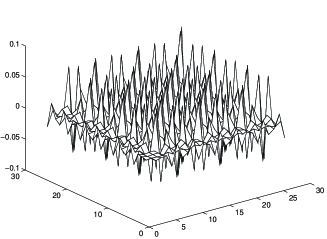
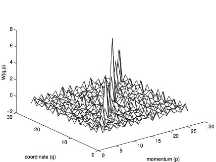
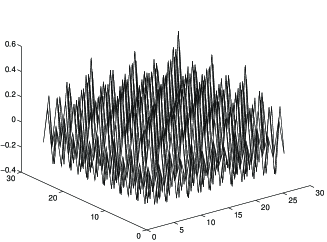
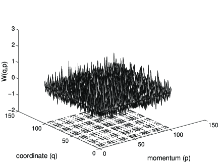
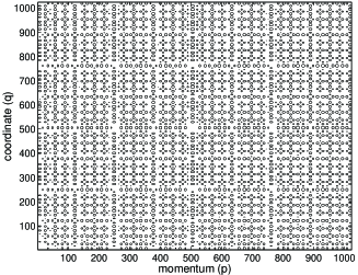
To classify the qualitative behaviour we apply standard methods from general control theory or really use the control. We will start from a priori unknown coefficients, the exact values of which will subsequently be recovered. Roughly speaking, we will fix only class of nonlinearity (polynomial in our case) which covers a broad variety of examples of possible truncation of the systems. As a simple model we choose band-triangular non-sparse matrices $(a_{ij})$ . These matrices provide tensor structure of bases in (extended) phase space and are generated by the roots of the reduced variational (Galerkin-like) systems. As a second step we need to restore the coefficients from these matrices by which we may classify the types of behaviour. We start with the localized mode, which is a base mode/eigenfunction, (Fig. 1, 9, 10 from Part I), corresponding to definitions from Section 2.2, Part I, which was constructed as a tensor product of the two Daubechies functions. Fig. 1, 4 below demonstrate the result of summation of series (67) up to value of the dilation/scale parameter equal to four and six, respectively. It’s done in the bases of symmlets [10] with the corresponding matrix elements equal to one. The size of matrix of “Fourier-wavelet coefficients” is 512x512. So, different possible distributions of the root values of the generical algebraical systems (66) provide qualitatively different types of behaviour. Generic algebraic system (66), Generalized Dispersion Relation (GDR), provide the possibility for algebraic control. The above choice provides us by a distribution with chaotic-like equidistribution. But, if we consider a band-like structure of matrix $(a_{ij})$ with the band along the main diagonal with finite size ( $\ll 512$ ) and values, e.g. five, while the other values are equal to one, we obtain localization in a fixed finite area of the full phase space, i.e. almost all energy of the system is concentrated in this small volume. This corresponds to waveleton states and is shown in Fig. 2, constructed by means of Daubechies-based wavelet packets. Depending on the type of solution, such localization may be conserved during the whole time evolution (asymptotically-stable) or up to the needed value from the whole time scale (e.g. enough for plasma fusion/confinement in the case of fusion modeling by means of c-BBGKY hierarchy for dynamics of partitions).

4 CONCLUSION

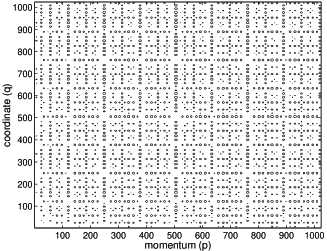
So, by using wavelet bases with their best (phase) space/time localization properties we can describe the localized (coherent) structures in quantum systems with complicated behaviour (Fig. 1, 4). The modeling demonstrates the formation of different (stable) pattern or orbits generated by internal hidden symmetry from high-localized structures. Our (nonlinear) eigenmodes are more realistic for the modelling of nonlinear classical/quantum dynamical process than the corresponding linear gaussian-like coherent states. Here we mention only the best convergence properties of the expansions based on wavelet packets, which realize the minimal Shannon entropy property and the exponential control of convergence of expansions like (67) based on the norm (45). Fig. 2 corresponds to (possible) result of superselection (einselection) [1] after decoherence process started from entangled state (Fig. 5); Fig. 3 and Fig. 6 demonstrate the steps of multiscale resolution during modeling of entangled states leading to the growth of degree of entanglement. It should be noted that we can control the type of behaviour on the level of the reduced algebraical variational system, GDR (66).

References

[1] D. Sternheimer, arXiv: math. QA/9809056; W. P. Schleich, Quantum Optics in Phase Space, Wiley, 2000; S. de Groot, L Suttorp, Foundations of Electrodynamics, North-Holland, 1972; W. Zurek, arXiv: quant-ph/0105127.
[2] A.N. Fedorova and M.G. Zeitlin, Math. and Comp. in Simulation, 46, 527, 1998; New Applications of Nonlinear and Chaotic Dynamics in Mechanics, Ed. F. Moon, 31, 101 Kluwer, Boston, 1998.
[3] A.N. Fedorova and M.G. Zeitlin, American Institute of Physics, Conf. Proc. v. 405, 87, 1997; arXiv: physics/9710035.
[4] A.N. Fedorova, M.G. Zeitlin, and Z. Parsa, AIP Conf. Proc. v. 468, 48, 69, 1999; arXiv: physics/990262, 990263.
[5] A.N. Fedorova and M.G. Zeitlin, The Physics of High Brightness Beams, Ed. J. Rosenzweig, 235, World Scientific, Singapore, 2001; arXiv: physics/0003095.
[6] A.N. Fedorova and M.G. Zeitlin, Quantum Aspects of Beam Physics, Ed. P. Chen, 527, 539, World Scientific, Singapore, 2002; arXiv: physics/0101006, 0101007.
[7] A.N. Fedorova and M.G. Zeitlin, Progress in Nonequilibrium Green’s Functions II, Ed. M. Bonitz, 481, World Scientific, Singapore, 2003; arXiv: physics/0212066; quant-phys/0306197.
[8] A.N. Fedorova and M.G. Zeitlin, Quantum Aspects of Beam Physics, Eds. Pisin Chen, K. Reil, 22, World Scientific, 2004, SLAC-R-630, Nuclear Instruments and Methods in Physics Research Section A, Volume 534, Issues 1-2, 309, 314, 2004; quant-ph/0406009, quant-ph/0406010, quant-ph/0306197.
[9] A.N. Fedorova and M.G. Zeitlin, Localization and Pattern Formation in Quantum Physics. I. Phenomena of Localization, this Volume.
[10] Y. Meyer, Wavelets and Operators, Cambridge Univ. Press, 1990.