Continuous variable private quantum channel

Abstract

In this paper we introduce the concept of quantum private channel within the continuous variables framework (CVPQC) and investigate its properties. In terms of CVPQC we naturally define a “maximally” mixed state in phase space together with its explicit construction and show that for increasing number of encryption operations (which sets the length of a shared key between Alice and Bob) the encrypted state is arbitrarily close to the maximally mixed state in the sense of the Hilbert-Schmidt distance. We bring the exact solution for the distance dependence and give also a rough estimate of the necessary number of bits of the shared secret key (i.e. how much classical resources are needed for an approximate encryption of a generally unknown continuous-variable state). The definition of the CVPQC is analyzed from the Holevo bound point of view which determines an upper bound of information about an incoming state an eavesdropper is able to get from his optimal measurement.

I Introduction

The task of quantum state encryption quant_ver_pad ; PQC ; encryption (quantum Vernam cipher, quantum one-time pad) is defined as follows. Let’s suppose that there are two communicating parties, Alice and Bob, and Alice wants to send an arbitrary unknown quantum state to Bob (the state needn’t to be known either Alice or Bob). They are connected through the quantum channel which is accessible to Eve’s manipulations. To avoid any possible information leakage from the state to Eve (via some kind of generalized measurement or state estimation) Alice and Bob share a secret and random string (classical key) of bits by which Alice chooses a unitary operation from the given (and publicly known) set. The transformed state is sent to Bob via the quantum channel who applies the same operation to decrypt the state. For an external observer (e.g. Eve) the state on the channel is a mixture of all possible transformations that Alice can create because she doesn’t know the secret string. If, moreover, the mixture is independent on the state to be encrypted then Eve has no chance to deduce any information on the state. We say that the state was perfectly encrypted. After the formalization of this procedure we get the definition of private quantum channel – PQC PQC . As the mixture it is advantageous to choose a maximally mixed state – identity density matrix.

It is natural to ask how many operations are needed for encryption of a $k$-qubit input state. Based on thoughts on entropy it was shown encryption and later generalized PQC for PQC with ancilla that $2k$ classical bits are sufficient (i.e. $2^{2k}$ operations). Generally, for perfect encryption of $d$-dimensional quantum state $d^{2}$ unitary operations are needed. Thus, the length of participant’s secret and random key must have at least $2\log d$ bits . After weakening the security definition an approximate secrecy was stated in approx_encryption defining of approximate private quantum channel – aPQC. Then, it was shown that asymptotically just $d\log d$ operations are needed for approximate quantum state encryption. Next progress in this research topic was achieved in approx_encryption1 where a polynomial algorithm for constructing a set of encryption/decryption operations suitable for aPQC was presented.

In this paper we investigate the possibility of quantum state encryption for continuous variables (CV) CV . Under CV we understand two conjugate observables such as e.g. position and momentum of a particle. Especially, we concentrate on coherent states states which Wigner function has the form of the normalized Gaussian distribution. Gaussian states are the most important class of CV states used in quantum communication and computation CV_prehled . The most of intriguing processes and algorithms discovered for discrete $d$-level quantum systems were also generalized for CV. Among others, let’s mention CV quantum state teleportation CV_tele1 ; CV_tele2 , CV quantum state cloning CV_clone and quantum computation with CV CV_comp . Importantly, a great progress was made in quantum key distribution (QKD) based on CV where theoretical groundwork was laid CV_crypto1 ; CV_crypto2 ; CV_crypto3 ; CV_crypto4 ; CV_crypto5 and experiments were performed CV_crypto_exp1 ; CV_crypto_exp2 .

After brief introducing into the questions of distances used in quantum information theory in Sec. II the main part follows in Sec. III and Sec. IV. There we present the notion of CV quantum state encryption and in the later we define a continuous-variable private quantum channel (CVPQC). This, foremost, consists of defining the “maximally” mixed state within the context of continuous variables and estimating the length of a secret shared key between Alice and Bob for a given secrecy (by secrecy it is meant the HS distance between “maximally” mixed and the investigated state). In Sec. IV we will touch the question of “maximality” of the mixed state (from now on, let’s omit the apostrophes) in the context of bosonic channels bos_chan1 ; bos_chan2 and their generalized lossy bos_chan_lossy and Gaussian relatives bos_gauss_chan_mem . We will also discuss important differences between discrete and CV encryption from the viewpoint of eavesdropping followed by the calculation of the Holevo bound limiting information accessible to Eve from the encrypted channel. Necessary Appendices come at the end of the paper. In Appendix A we give a derivation of the exact formula for the HS distance. The object of Appendix B is to inference the mentioned estimate of the HS distance.

II Measures of quantum states closeness

Quantum states can be distinguished in the sense of their mutual distance. The distance is usually induced by a norm defined on the space of quantum states. This is the case of Schatten $p$-norm

$$\|A\|_{p}=\left(\mathop{{\mathrm{Tr}}}\left(\left|A\right|^{p}\right)\right)^{\frac{1}{p}}=\left(\mathop{{\mathrm{Tr}}}\left(A^{p}\right)\right)^{\frac{1}{p}},$$ (1)

where $|A|=\sqrt{A^{\dagger}A}$ and the last equation is valid for $A=A^{\dagger}$. If $A=\varrho_{1}-\varrho_{2}$ the Hermiticity of $A$ is still preserved and for $p=2$ we get the Hilbert-Schmidt (HS) distance

$$D_{HS}(\varrho_{1},\varrho_{2})=\|\varrho_{1}-\varrho_{2}\|_{2}=\sqrt{\mathop{{\mathrm{Tr}}}\left((\varrho_{1}-\varrho_{2})^{2}\right)}.$$ (2)

On the other hand, there is a whole family of distances based on Uhlmann’s fidelity uhlmann

$$F(\rho_{1},\rho_{2})=\mathop{{\mathrm{Tr}}}\left(\left(\sqrt{\rho_{1}}\rho_{2}\sqrt{\rho_{1}}\right)^{\frac{1}{2}}\right).$$ (3)

One of them is Bures distance bures

$$D_{B}(\varrho_{1},\varrho_{2})=\left(2-2\mathop{{\mathrm{Tr}}}\sqrt{\sqrt{\varrho_{1}}\varrho_{2}\sqrt{\varrho_{1}}}\right)^{\frac{1}{2}}$$ (4)

which coincides with the HS distance if $\varrho_{1},\varrho_{2}$ are pure states.

There is a certain equivocation which distance is more suitable for a given task in QIT where a general problem of quantum state distinguishability or closeness has to be resolved. Both distances have many useful properties and they are subject of detailed investigation SommZyc . For example, output “quality” of a quantum state in the problem of universal quantum-copying machine was first analyzed with the help of the HS distance UQCM_HS and later revisited from the viewpoint of the Bures and trace distance (Schatten $p$-norm (1) for $p=1$) UQCM_Bures . Other problem, among others, where closeness of two quantum states plays a significant role is quantum state estimation quantstateest . Here the closeness of estimated states is often measured by the HS distance quantstateest_HS .

The motivation for using the HS distance in our calculation is two-fold. First, the security criterion for approximate quantum state encryption approx_encryption is based on the operator distance induced by operator norm ($p\to\infty$ in (1)) while some other results therein are calculated for the trace distance which is in some sense weaker than the operator distance (the reason is computational difficulty). Second, for our purpose we need to calculate distance between two infinitely-dimensional mixed states what is difficult in the case of all fidelity based distances. However, we suppose that the HS distance is a good choice for coherent states and provides an adequate view on measure of the closeness of two states.

III CV state encryption and its analysis

Let’s define the task of CV state encryption. As in the case of discrete variable quantum state encryption, Alice and Bob are interconnected via a quantum channel which is fully accessible to Eve’s manipulations. Both legal participants share a secret string of random bits (key) which sufficient length is, among others, subject of this paper. The key indexes several unitary operations which Alice/Bob chooses to encrypt/decrypt single-mode coherent states. The purpose of the encryption is to secure these states from leakage of any information about them to an eavesdropper (Eve). The way to achieve this task is to “randomize” every coherent state to be close as much as possible to a maximally mixed state (maximally in the sense specified next). The randomization is performed with several publicly known unitary operations (it is meant that the set from which participants choose is known but the particular sequence of operations from the set is given by the key which is kept secret). So, suppose that Alice generates or gets an arbitrary and generally unknown single-mode coherent state. The only public knowledge about the state is its appearance somewhere inside the circle of radius $b$ in phase space with the given distribution probability. Here we suppose that states occur with the same probability for all $r\leq b$ and with zero probability elsewhere.

Suppose for a while that Alice encrypts a vacuum state. This situation will be immediately generalized with the help of the HS distance properties for an unknown coherent state within the circle of radius $b$ as stated in the previous paragraph. The first problem we have to tackle is the definition of a maximally (or completely) mixed state. Here the situation is different from, generally, $d$-dimensional discrete Hilbert space where a normalized unit matrix is considered as the maximally mixed state. This is inappropriate in phase space nevertheless we may inspire ourselves in a way the discrete maximally mixed state is generated. In fact, we get the maximally mixed state (in case of qubits $\varrho_{V}=\varrho_{r\vartheta\varphi}$) by integrating out over all density matrix populating the Bloch sphere $\openone\propto\int\varrho_{V}{\rm d}V$ (irrespective of the fact that the finite number of unitary operations suffice for this task as the theory of PQC learns). Similarly, as a maximally mixed state  we can naturally choose an integral performed over all possible single-mode states within the circle of radius $r\leq b$

$$\openone_{b} =\frac{1}{C}\int{\rm d}^{2}\alpha|\alpha\rangle\!\langle\alpha|=\frac{1}{C}\sum_{m,n=0}^{\infty}|m\rangle\!\langle n|\int_{0}^{2\pi}{\rm d}\vartheta\int_{0}^{b}{\rm d}r\ e^{-r^{2}}\frac{r^{m+n+1}}{\sqrt{m!n!}}e^{i(m-n)\vartheta}=\frac{2\pi}{C}\sum_{n=0}^{\infty}\frac{|n\rangle\!\langle n|}{n!}\int_{0}^{b}{\rm d}r\ e^{-r^{2}}r^{2n+1}$$

$$=\frac{\pi}{C}\sum_{n=0}^{\infty}\frac{|n\rangle\!\langle n|}{n!}\int_{0}^{b^{2}}{\rm d}x\ e^{-x}x^{n}=\frac{\pi}{C}\exp\left(-b^{2}\right)\sum_{n=0}^{\infty}\left(\exp\left(b^{2}\right)-\sum_{k=0}^{n}\frac{b^{2k}}{k!}\right)|n\rangle\!\langle n|.$$ (5)

$\mathop{\left|\alpha\right>}\nolimits=D(\alpha)\mathop{\left|0\right>}\nolimits=\exp(-|\alpha|^{2}/2)\sum_{n=0}^{\infty}\frac{\alpha^{n}}{\sqrt{n!}}\mathop{\left|n\right>}\nolimits$ is a coherent state represented as a displaced vacuum via the displacement operator $D(\alpha)$ (from now on it will not be mentioned explicitly that $|\alpha|\leq b$ for all displacement operators used in this paper and for given $b$) and $C=\pi b^{2}$ is a normalization constant. Note that calculation (III) for $b\to\infty$ without the normalization is nothing else than well known resolving of unity giving the evidence of spanning the whole Hilbert space.

Having defined the maximally mixed state let’s investigate which operations Alice uses for encryption. This transformation should be as close as possible to the maximally state in the HS distance sense and the closeness will depend on the number of used operations. Beforehand, we will note how to facilitate forthcoming tedious calculations on a sample example. Suppose that Alice has e.g. four encryption operations, which displace the vacuum state to the same distance $r_{4}$ from the origin but under four different angles (from symmetrical reason these angles are multiples of $\frac{\pi}{2}$ in this case). Alice chooses these operations with the same probability. Now, if we write down the overall mixture from the states, it can be shown that there exists a computationally advantageous “conformation” when the mixture reads

$$\varrho_{4}=\frac{1}{4}\sum_{q=1}^{4}|\alpha_{4q}\rangle\!\langle\alpha_{4q}|=\exp(-r_{4}^{2})\sum_{m,n=0}^{\infty}\frac{r_{4}^{m+n}}{\sqrt{m!n!}}|m\rangle\!\langle n|\,\delta_{m}^{m^{\prime}},$$ (6)

where $m^{\prime}=m+4l$, $l=1,\dots,\infty$ and $\delta_{m}^{m^{\prime}}=1$ for all $m$ (occupation number) else $\delta_{m}^{m^{\prime}}=0$. Informally, (6) is always a real density matrix with off-diagonal non-zero “stripes” separated from main diagonal and from a neighbouring stripe by three zero off-diagonals. $\varrho_{4}$ acquires relatively simple form (6) if $\alpha_{4q}=r_{4}e^{iq\vartheta_{4q}}$ for $\vartheta_{4q}=\frac{\pi}{4}+(q-1)\frac{\pi}{2}$. This can be generalized for arbitrary number of states dispersed on a circle with given radius $r_{p}$

$$\varrho_{p}=\frac{1}{p}\sum_{q=1}^{p}|\alpha_{pq}\rangle\!\langle\alpha_{pq}|=\exp(-r_{p}^{2})\sum_{m,n=0}^{\infty}\frac{r_{p}^{m+n}}{\sqrt{m!n!}}|m\rangle\!\langle n|\,\delta_{m}^{m^{\prime}},$$ (7)

where $p\in{\mathbb{Z}}^{+}$,$m^{\prime}=m+pl$ and $\delta_{m}^{m^{\prime}}$ is defined as before. Favorable “$p$-conformations” (7) occur when $\alpha_{pq}=r_{p}e^{iq\vartheta_{pq}}$ for $\vartheta_{pq}=\frac{\pi}{p}(2q-1)$. Now, we may proceed to the mixture characterizing all Alice’s encryption operations. She chooses $N\geq 1$ and defines $r_{p}=pb/N$ for $p=1,\dots,N$. Then

$$\Phi_{N}=\frac{1}{M}\sum_{p=1}^{N}p\varrho_{p}=\frac{1}{M}\sum_{p=1}^{N}\sum_{q=1}^{p}D(\alpha_{pq})|0\rangle\!\langle 0|D^{\dagger}(\alpha_{pq})$$ (8)

with normalization $M=\frac{N(N+1)}{2}$. To sum up the protocol, Alice and Bob share a secret and random key which indexes their operations. So, Alice equiprobably chooses from the set of $M$ displacement operators $D(\alpha_{pq})=\exp(\alpha_{pq}a^{\dagger}-\alpha_{pq}^{*}a)$ where just one operator creates a coherent state on the circle of radius $r_{1}$, two operators generate two states on the circle of radius $r_{2}$ and so forth up to $N$. Mixtures of the states on particular circles are in favourable form (7) and the whole state is (8). The rest of the protocol is the same as in discrete state encryption. Alice sends the encrypted state through a quantum channel towards Bob who makes Alice’s inverse operation to decrypt the state.

The keystone in quantum state encryption both discrete and CV is the fact that an unknown and arbitrary state can be encrypted. If the state was known we would’t need this procedure at all because Alice could just send information about the preparation of the state to Bob. So, it would suffice to encrypt this classical information with the Vernam cipher. Also, our definition of CVPQC must be independent on the state which is to be encrypted. To provide this we will find useful unitary invariance of the HS distance $D_{HS}(\varrho,\sigma)=D_{HS}(U\varrho U^{\dagger},U\sigma U^{\dagger})$ for an arbitrary unitary matrix $U$. This invariance is, however, necessary but not sufficient condition for our purpose. The second important issue is due to advantageous algebraic properties of displacement operators. Let’s demonstrate it on Alice’s encryption algorithm which stays the same as before. If she gets an arbitrary coherent state $\mathop{\left|\beta\right>}\nolimits$ ($|\beta|\leq b$) she randomly chooses one from $M$ displacement operators $D(\alpha_{pq})$ (as the shared key with Bob dictates). Then, even if two displacement operators generally do not commute we may write a general encryption TPCP (trace-preserving completely positive) map

$$\mathcal{E}_{N}(\mathop{\left|\beta\right>}\nolimits)=\frac{1}{M}\sum_{p=1}^{N}\sum_{q=1}^{p}D(\alpha_{pq})D(\beta)|0\rangle\!\langle 0|D^{\dagger}(\beta)D^{\dagger}(\alpha_{pq})=\frac{1}{M}\sum_{p=1}^{N}\sum_{q=1}^{p}D(\beta)D(\alpha_{pq})|0\rangle\!\langle 0|D^{\dagger}(\alpha_{pq})D^{\dagger}(\beta)=D(\beta)\Phi_{N}D^{\dagger}(\beta).$$ (9)

It is obvious that generally $\mathcal{E}_{N}(\mathop{\left|\beta\right>}\nolimits)\not=\Phi_{N}$ (and similarly $\int D(\alpha)|\beta\rangle\!\langle\beta|D^{\dagger}(\alpha){\rm d}^{2}\alpha\propto D(\beta)\openone_{b}D^{\dagger}(\beta)=\openone_{b}^{\beta}\not=\openone_{b}$) but their HS distances are equivalent, i.e. $D_{HS}(\openone_{b}^{\beta},\mathcal{E}_{N}(\mathop{\left|\beta\right>}\nolimits))=D_{HS}(\openone_{b},\Phi_{N})$. Thus, we are henceforth entitled to make all calculations of the HS distance between $\openone_{b}^{\beta}$ and $\mathcal{E}_{N}(\mathop{\left|\beta\right>}\nolimits)$ with explicit forms (III) and (8). After some calculations we will see (Appendix B) that

$$D_{HS}^{2}\left(\openone_{b}^{\beta},\mathcal{E}_{N}(\mathop{\left|\beta\right>}\nolimits)\right)\approx\left(\frac{1}{N+1}\right)^{2}+\mathcal{O}\left(N^{-4}\right),$$ (10)

which holds for all for all input coherent states $\mathop{\left|\beta\right>}\nolimits$. The guess (10) is far from optimal (e.g. independent on $b$) and is not even an inequality. But this doesn’t matter because the exact form can be derived (for details see Appendix A). Its only problem is relative complexity so we cannot easily deduce the number of operations for a given level of secrecy. Nevertheless, (10) asymptotically approaches to the exact expression (as is shown in Appendix B). Notice that in spite of the derivation of (10) (or, next, analytical expression (III)) we still cannot reasonably define a CVPQC. We will do so in section IV after presenting another assumptions regarding eavesdropping on our private quantum channel.

If we consider the described unitary invariance of the HS distance we write down lhs of (10)

$$D_{HS}^{2}(\openone_{b},\Phi_{N})=\mathop{{\mathrm{Tr}}}\left((\openone_{b}-\Phi_{N})^{2}\right)=\mathop{{\mathrm{Tr}}}\left(\openone_{b}^{2}\right)-2\mathop{{\mathrm{Tr}}}\left(\openone_{b}\Phi_{N}\right)+\mathop{{\mathrm{Tr}}}\left(\Phi_{N}^{2}\right).$$ (11)

After some calculations (see mentioned Appendix A) we get a little bit lengthy expression

$$D_{HS}^{2}(\openone_{b},\Phi_{N}) =\frac{1}{b^{2}\exp(2b^{2})}\left(\exp(2b^{2})-I_{0}\left(2b^{2}\right)-I_{1}\left(2b^{2}\right)\right)-\frac{4\exp(-b^{2})}{b^{2}N(N+1)}\sum_{p=1}^{N}\frac{p}{\exp\left(r_{p}^{2}\right)}\sum_{k=1}^{\infty}\left(\frac{b}{r_{p}}\right)^{k}I_{k}(2r_{p}b)$$

$$+\left(\frac{2}{N(N+1)}\right)^{2}\left[\sum_{p=1}^{N}\frac{p^{2}}{\exp\left(2r_{p}^{2}\right)}\left(I_{0}\left(2r_{p}^{2}\right)+2\sum_{k=1}^{\infty}I_{pk}\left(2r_{p}^{2}\right)\right)\right.$$

$$+\sum_{\genfrac{}{}{0.0pt}{}{p_{1},p_{2}=1}{p_{1}\not=p_{2}}}^{N}\frac{p_{1}p_{2}}{\exp\left(r_{p_{1}}^{2}+r_{p_{2}}^{2}\right)}\left.\left(I_{0}(2R_{12})+2\sum_{k=1}^{\infty}I_{p_{1}p_{2}k}(2R_{12})\right)\right],$$ (12)

where $r_{p}=pb/N,r_{p_{l}}=p_{l}b/N,R_{12}=p_{1}p_{2}\left(b/N\right)^{2}$ and $I_{n}(x)$ is a modified Bessel function of the first kind of order $n$

$$I_{n}(x)=\sum_{s=0}^{\infty}{\left(\frac{x}{2}\right)^{n+2s}}\frac{1}{(n+s)!s!}.$$ (13)

However, as we declared, for a rough estimation of the number of operations for a given secrecy we will employ (10). Using $M=\frac{N(N+1)}{2}\approx\frac{(N+1)^{2}}{2}$ (and then again $M\approx\frac{N^{2}}{2}$) we find that the dependence of the number of bits on the HS distance (III) is $n=\log M=-2(1+\log D_{HS})+\log\left(1+\sqrt{1+CD_{HS}^{2}}\right)\approx-1-2\log D_{HS}$ because the guess is in particular precise for $D_{HS}\ll 1$. $C$ is a constant (polynomial) bounding $N^{-4}$ in (10) from above. By the numerical simulations based on (III) for different $b$ and $M$ we see that the guess is accurate and for higher $M$ even serves as a relatively good upper bound.

Simplified encryption

Now, let’s see what is going to happen if we simplify our encryption protocol. The arrangement is the same, i.e. Alice’s task is to encipher single-mode coherent states and her only knowledge is that the states are somewhere inside the circle of radius $r\leq b$. However, Alice’s technology is limited and we will tend to replace technologically demanding displacements by simple phase shifts given by the well known time evolution $\mathop{\left|\alpha(t)\right>}\nolimits=\exp(-iHt/\hbar)\mathop{\left|\alpha\right>}\nolimits$ with the Hamiltonian $H=\hbar\omega(n+\frac{1}{2})$. The resulting state is $\mathop{\left|\alpha(t)\right>}\nolimits=\exp(-i\omega t/2)\mathop{\left|\alpha\exp(-i\omega t)\right>}\nolimits$ so the state undertakes the rotation about $\Theta=\omega t$ regardless the distance (which stays preserved) from the phase space origin. Note that unitary operator $U=\exp(-iHt/\hbar)$ has the form

$$U=\exp\left(-\frac{i\omega t}{2}\right)\sum_{n=0}^{\infty}\exp(-i\omega tn)|n\rangle\!\langle n|.$$ (14)

Next, suppose that Alice is equipped with $p$ encryption operations where she can rotate the state about $q$ multiples of $2\pi/p$. So, $\Theta_{q}=q2\pi/p$ where $q=1,\dots,p$. Then, for someone without any information about the angle of rotation chosen by Alice (e.g. Eve) the state leaving Alice is in the form

$$\tilde{\varrho}_{p}=\frac{1}{p}\sum_{q=1}^{p}U_{q}|\alpha\rangle\!\langle\alpha|U^{-1}_{q}=\frac{1}{p}\sum_{q=1}^{p}\left(|\alpha\rangle\!\langle\alpha|\right)_{q}=\frac{1}{p}\sum_{q=1}^{p}|\alpha e^{\frac{q2\pi}{p}}\rangle\!\langle\alpha e^{\frac{q2\pi}{p}}|$$ (15)

where $U_{q}$ is (14) with $\Theta_{q}=\omega t_{q}=q2\pi/p$. Because Alice doesn’t know where exactly the state $\mathop{\left|\alpha\right>}\nolimits$ is placed we cannot write an explicit form of $\tilde{\varrho}_{q}$. Apparently, however, for arbitrary $p$ it can be transformed to our favourite state (7), again with the help of unitary operation (14)

$$\varrho_{p}(r_{p})=U\tilde{\varrho}_{p}U^{-1}=\exp(-r_{p}^{2})\sum_{m,n=0}^{\infty}\frac{r_{p}^{m+n}}{\sqrt{m!n!}}|m\rangle\!\langle n|\,\delta_{m}^{m^{\prime}},$$ (16)

where $m^{\prime}=m+pl$, $l=1,\dots,\infty$. It remains to show that $\openone_{b}=U\openone_{b}U^{-1}$. This can be readily seen from the fact that (14) is diagonal. This is vital. Now we can easily calculate the HS distance of $\varrho_{p}(r_{p})$ and $\openone_{b}$ and regarding the unitary invariance of the HS distance the result will be valid for any arbitrary input coherent state (this trick is akin to that one used in (9)). After the calculation we get the same result as in (III) but for fixed $p$ and without the summation over $p_{1},p_{2}$

$$D_{HS}^{2}(\openone_{b},\varrho_{p}) =\frac{1}{b^{2}\exp(2b^{2})}\left(\exp(2b^{2})-I_{0}\left(2b^{2}\right)-I_{1}\left(2b^{2}\right)\right)-\frac{2}{\exp\left(b^{2}\right)b^{2}}\frac{1}{\exp\left(r_{p}^{2}\right)}\sum_{k=1}^{\infty}\left(\frac{b}{r_{p}}\right)^{k}I_{k}(2r_{p}b)$$

$$+\frac{1}{\exp\left(2r_{p}^{2}\right)}\left(I_{0}\left(2r_{p}^{2}\right)+2\sum_{k=1}^{\infty}I_{pk}\left(2r_{p}^{2}\right)\right).$$ (17)

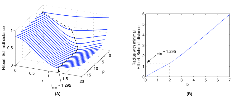
Figure 1: (A) In the case of technologically simplified encryption Alice has at disposal just one displacement operator and several phase shifts. The depicted HS distances (III) (here for $b=2$ and $p=1,\dots,20$ determining the number of used encryption operations) illustrates how Alice chooses the proper displacement $D(r_{min})$ and a correct number of phase shifts. We see that for $p\gtrsim 6$ the minimum is “saturated” so Alice needs just six phase shifts for the best approximation to full-encryption protocol. Another rising of $p$ doesn’t bring any advantage. The dash-dotted curve connects minima for their better visibility. (B) Numerical solutions of Eq. (18) for different $b$ (i.e. growing input range of states coming to Alice) tells us which displacement is needed in the case of simplified encryption. For these values of $r_{min}$ the HS distance (III) reaches the lowest values. A special case of $b=2$ is highlighted to see its correspondence with the picture on the left.

The behaviour of this quantity is completely different compared to (III) describing the original case as can be seen in Fig. 1 (A). As an example we put $b=2$ and we see that there exists $r_{min}<b$ for which the HS distance between (III) and (16) reaches its minimum for sufficiently high $p$. In order to find a radius minimizing the HS distance of these density matrices for various $b$ (we put $p\to\infty$ and thus $2\sum_{k=1}^{\infty}I_{pk}\left(2r_{p}^{2}\right)$ vanishes – we seek for, say, a saturated minimum which is independent on the number of operations on a given circle) we can calculate

$$\frac{\partial\left(D_{HS}^{2}(\openone_{b},\varrho_{p})\right)}{\partial r}\stackrel{{\scriptstyle p\to\infty}}{{=}}\frac{4}{\exp\left(2r_{min}^{2}\right)}\left(r_{min}I_{1}\left(2r_{min}^{2}\right)-r_{min}I_{0}\left(2r_{min}^{2}\right)+\frac{\exp\left(2r_{min}^{2}\right)}{b\exp\left(b^{2}\right)}I_{1}\left(2r_{min}b\right)\right)=0.$$ (18)

The solution is the root of the expression in parentheses. Unfortunately, an analytical solution wasn’t found so numerical calculation of $r_{min}$ for several $b\in\left(0,7\right.\rangle$ is depicted in Fig. 1 (B).

What are the physical consequences of this whole simplification? From Fig. 1 (A) we see that a maximally mixed state $\openone_{b}$ can be in the distance sense substituted with a mixture of coherent state on a circle (with radius $r_{min}$ where the diversion from $\openone_{b}$ is smallest) and the mixing requires relatively few encryption operations (low $p$ for the distance saturation). It holds not only for $b=2$ what is the case in the picture. So, now we can make the process of encryption/decryption technologically easier. We equip Alice/Bob with mentioned phase shifts leading to (16) and just one displacement operator $D(r_{min})$. Every incoming coherent state is first displaced and then encrypted by choosing a phase shift (indexed by a secret key). The role of Fig. 1 (B) is in a proper choice of $r_{min}$ for given $b$. Finally, Alice examines Fig. 1 (A) to select a sufficient number $p$ of phase shifts for which the minimum of HS distance (III) stays essentially the same.

The important point is that incoming coherent states come to Alice randomly and equiprobably for given $b$ so after this simplified encryption (and for many encryption instances) they are as close as possible to full-fashioned encrypted states as they would be if processed by using (8), i.e. the case of fully technologically equipped Alice and Bob, respectively. The overall advantage is the use of just one technologically demanding operation which doesn’t need to be tuned for given $b$ (it stays fixed in the encryption protocol described at the beginning of chapter III).

IV Eavesdropping on encrypted CV states

Quantum channels are TPCP maps on quantum states. Following the classical channel coding theorem shannon48 one may ask how much information is a quantum channel able to convey. This question naturally leads to the definition of quantum channel capacity (for a nice survey on various quantum channel capacities see Ref. shor_capa ) as the maximum of the accessible information over the probability distributions of the input states ensemble $\{p_{i},\sigma_{i}\}$ entering the channel (after classical-quantum coding onto input quantum states $x_{i}\rightleftharpoons\sigma_{i}$ the ensemble of classical messages is indicated by the variable $X=\{p(x_{i}),x_{i}\}$ where $p(x_{i})\equiv p_{i}$). The accessible information $I_{acc}$ itself is the maximization over all measurement of the mutual information $I(X;Y)$ with the variable $Y=\{p\,(y_{j}),y_{j}\}$ giving the probability $p\,(y_{j})$ of the result $y_{j}$ (an output alphabet) of a measurement on the channel output. Sometimes it might be difficult to calculate the accessible information to determine the channel capacity. Then, we can estimate the accessible information from above by the Holevo bound

$$\chi\left(\{p_{i},\sigma_{i}\}\right)=S\biggl{(}\sum_{i}p_{i}\sigma_{i}\biggr{)}-\sum_{i}p_{i}S(\sigma_{i}),$$ (19)

for which was proved holevo_bound that $\chi\geq I_{acc}$ ($S(\varrho)$ is the von Neumann entropy) reaching equality if all $\sigma_{i}$ commute.

In our case we try to get as close as possible to our maximally mixed state (III) with TPCP map (8) (or, generally, to $\openone_{b}^{\beta}$ with (9)) which both belong to the class of bosonic channels bos_chan1 ; bos_chan2 . However, our task is quite different from reaching the highest quantum channel capacity (what means “tuning” of $p_{i}$). Now, the variable $X$ is fixed. For our purpose the Holevo bound can tell us what is the upper bound on information which is a third party (Eve) able to learn from her very best (that is optimal) measurement on the quantum channel. The question now is of what state we should calculate the Holevo bound to find Eve’s maximum of attainable information on incoming states. Unlike the discrete case (perfect and approximate encryption) the condition of perfect and acceptable closeness of an encrypted state to the maximally mixed state is not in this case sufficient. Let’s demonstrate the reason for this difference on the Bloch sphere (i.e. perfect qubit encryption). If Alice encrypts an unknown qubit (with a PQC compound from e.g. four Pauli matrices) she gets a maximally mixed two-qubit state (normalized unity matrix). It means that Eve cannot construct any measurement giving her information on the state. Moreover, even if she had a priori information on the state (in the sense that Alice gets and encrypts many copies of the same unknown state) she wouldn’t be able to use any method of unknown quantum states reconstruction quantstateest . She wouldn’t get any clue where to find the state because all are transformed (encrypted) to the maximally mixed state dwelling in the center of the sphere. Unfortunately, this is not our case. Here, if Alice encrypts many identical coherent states (howbeit unknown) Eve could in principle reconstruct in which part of the phase space the encryption had been carried out. Because we next suppose that encryption operations are publicly known (naturally not the secret key sequence itself) Eve then could be able to deduce the original state from many variant ciphers of the same state. So we will suppose that incoming state do not exhibit such statistics and, moreover, they are distributed equiprobably and randomly in the whole region of considering (i.e. within the circle of radius $r\leq b$) . Less restrictive requirement could be a distribution independent on the phase and changing only with the distance from the origin (rotationally invariant) what will be discussed at the end of this chapter.

Based on theses thoughts, we may finally define CVPQC. We call the object $\{\mathcal{B},P_{\mathcal{B}},\mathcal{E}_{N}(\mathop{\left|\beta\right>}\nolimits),\openone_{b}^{\beta}\}$ as CVPQC where $\mathcal{B}$ is the set of all coherent states $\mathop{\left|\beta\right>}\nolimits$ ($|\beta|\leq b$) with distribution $P_{\mathcal{B}}$ around the origin of phase space, $\mathcal{E}_{N}(\mathop{\left|\beta\right>}\nolimits)$ is the TPCP map defined in (9) and $\openone_{b}^{\beta}$ is maximally mixed state centered around an input state $\mathop{\left|\beta\right>}\nolimits$ (displaced (III)). Let’s note that the definition of CVPQC is valid for all coherent mixed states of the general form $\varrho_{\beta}=\sum_{i}p_{i}(|\beta\rangle\!\langle\beta|)_{i}$ with $\sum_{i}p_{i}=1$ and $|\beta|_{i}\leq b,\,\forall i$ because of convexity of HS norm. The situation is similar as in approx_encryption for the operator norm.

Considering the assumptions from the previous paragraph let’s focus on the problem of security on the channel. For our purpose we employ an integral version of (19). First note that we are now interested in the limiting case when Alice uses infinitely many encryption operations . More importantly, it remains to correctly answer the question posed above. That is, what actually calculate as the Holevo bound? We know that Eve will measure on the encrypted channel to get any information on incoming states (states before the encryption). To learn something about position of a coherent state before encryption Eve must try to distinguish among objects which preserve some information about input states location in phase space. In other words Eve has to choose a correct “encoding” $\sigma_{i}$ from Eq. (19) but now for a continuous index. Due to the used encryption operation (9) (which in our case $N\to\infty$ transforms to $\openone_{b}^{\beta}$ as is proved in Appendix A) a state $\openone_{b}^{\beta}$ is that object which preserves the information on placement of an incoming state $\mathop{\left|\beta\right>}\nolimits$ because is centered around it. Then, a continuous version of (19) reads

$$\chi\bigl{(}\{P(\beta),\openone_{b}^{\beta}\}\bigr{)}=S\bigl{(}\tilde{\Lambda}_{2b}\bigr{)}-\int{\rm d^{2}}\beta\,P(\beta)S\bigl{(}\openone_{b}^{\beta}\bigr{)},$$ (20)

where $\tilde{\Lambda}_{2b}$ is a total state leaving Alice’s apparatus (normalized Eq. (IV)), $P(\beta)$ is an input distribution from the CVPQC definition and $\openone_{b}^{\beta}=D(\beta)\openone_{b}D^{\dagger}(\beta)$. Since $S(D(\beta)\openone_{b}D^{\dagger}(\beta))=S(\openone_{b})$ for all $\beta$ it immediately follows from (20)

$$\chi\left(\{P(\beta),\openone_{b}^{\beta}\}\right)=S\bigl{(}\tilde{\Lambda}_{2b}\bigr{)}-S\bigl{(}\openone_{b}\bigr{)}.$$ (21)

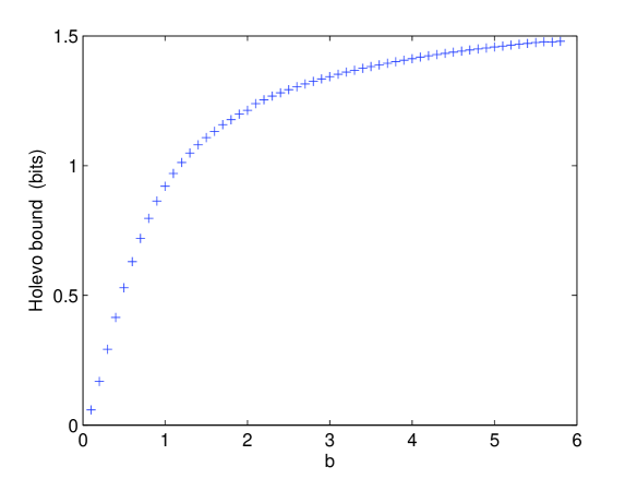
Figure 2: The Holevo bound represents an upper bound for information Eve is able to get from her best measurement on the encrypted channel. The bigger is the set of states coming to Alice (growing $b$) the more information Eve can extract. This is caused by better discriminability of Eve’s measuring apparatus. Nevertheless, relatively low calculated values of the Holevo bound for our CVPQC given by Eq. (21) limits Eve in eavesdropping on the channel.

To calculate the Holevo bound (21) it remains to find the total state after the encryption procedure provided that Eve doesn’t know neither which particular coherent state $\mathop{\left|\beta\right>}\nolimits$ comes to Alice nor the key used for encryption. Thus, because the incoming distribution $P(\beta)\equiv P(x,\vartheta)=1$ (no need to normalize it here) is publicly known then Alice quite accidentally experiences $\openone_{b}$ also as a total incoming state. So, the state leaving Alice is in the form

$$\Lambda_{2b} =\int{\rm d^{2}}\alpha D(\alpha)\left(\int{\rm d^{2}}\beta\,|\beta\rangle\!\langle\beta|\right)D^{\dagger}(\alpha)=\int_{0}^{b}\int_{0}^{2\pi}{\rm d^{2}}\beta\left(\int_{0}^{b}\int_{0}^{2\pi}{\rm d^{2}}\alpha\,D(\alpha)|\beta\rangle\!\langle\beta|D^{\dagger}(\alpha)\right)$$

$$=\int_{0}^{b}x{\rm d}x\int_{0}^{b}y{\rm d}y\int_{0}^{2\pi}{\rm d}\varphi\left(\int_{0}^{2\pi}{\rm d}\vartheta\,|\beta+\alpha\rangle\!\langle\beta+\alpha|\right)=2\pi\sum_{n=0}^{\infty}\frac{|n\rangle\!\langle n|}{n!}\int_{0}^{b}\int_{0}^{b}\int_{0}^{2\pi}{\rm d}x{\rm d}y{\rm d}\varphi\ e^{-R^{2}}R^{2n+1}xy,$$ (22)

where $R^{2}=x^{2}+y^{2}-2xy\cos\varphi\leq 4b^{2}$, ${\rm d^{2}}\alpha=y{\rm d}y{\rm d}\varphi$, ${\rm d^{2}}\beta=x{\rm d}x{\rm d}\vartheta$ and $D(\alpha)$ are encryption displacements (again uniformly distributed as the CVPQC definition dictates and without a normalization). Shortly said, by changing the order of integration we see that $\Lambda_{2b}$ is diagonal. Concretely, the term in the parentheses in the reordered integral (second row in (IV)) is an ordinary coherent state $\mathop{\left|\beta+\alpha\right>}\nolimits$ ($r$ is its distance from the origin and abscissae formed by points in the phase space $(\alpha,\beta)$ and $(\beta,0)$ contain a relative angle $\varphi$) and is integrated out over the phase. This gives a diagonal matrix and next integrating just changes the statistics on the diagonal. Note that $\Lambda_{2b}$ “covers” the area of radius $2b$ in phase space. Unfortunately, it is difficult to obtain an analytical solution of (IV). Nevertheless, based on (IV) we may generally write (tilde indicates normalization) $\tilde{\Lambda}_{2b}=\sum_{n}\lambda^{(b)}_{n}|n\rangle\!\langle n|$, where $\lambda^{(b)}_{n}$ are needed to be determined numerically. Inserting $\tilde{\Lambda}_{2b}=\sum_{n}\lambda^{(b)}_{n}|n\rangle\!\langle n|$ and (III) into Eq. (21) we find the desired Holevo bound what is depicted in Fig. 2. It is interesting to note that the convergence of the Holevo bound is tightly connected with the energy constraint $\int\mathop{{\mathrm{Tr}}}\left(\varrho_{\beta}a^{\dagger}a\right){\rm d}P_{\mathcal{B}}\leq\bar{n}_{b}$ which is automatically satisfied through the finiteness of $b$ in our CVPQC. For a general distribution $P(\beta)$ it is satisfied due to the natural condition $\int{\rm d^{2}}\beta P(\beta)=1$. The importance of the constraint has been already recognized for capacities of bosonic channels bos_chan1 ; bos_chan2 ; bos_chan_lossy ; bos_gauss_chan_mem .

From Fig. 2 we see that there is no chance for Eve to find which coherent state actually passes on the channel. This is not so surprising considering the non-discrete character of the input distribution $P(\beta)$. But Eve cannot divide the appropriate area at least roughly to approximately devise the position of a particular encrypted state $\openone_{b}^{\beta}$ (and from this to derive the desired position of an incoming state $\mathop{\left|\beta\right>}\nolimits$). From the informational point of view the Holevo bound results could be interpreted such that for a given $b$ there doesn’t exist any optimal measurement enabling Eve to divide the circle of the radius $2b$ in more than $2^{\chi}$ sections and tells her in which one the encrypted state occurs.

Having fixed the input distribution $P(\beta)$ of coherent states coming to Alice another way how to next decrease the Holevo bound might be a different definition of an encryption distribution in Eq. (IV) where a uniform distribution is implicitly used. If this distribution was symmetrical (i.e. rotationally invariant, for example Gaussian one) then we would find Eq. (IV) diagonal as well and thus we could easily calculate (21). However, a big challenge is proving the optimality of such distribution function. Anyhow, it means that by minimizing the Holevo bound (21) within the context of the CVPQC definition we could tackle the previously mentioned problem of maximality of our mixed state by putting this more suitable distribution into Eq. (III).

V Conclusion

In this work we have opened the problem of continuous variable encryption of unknown quantum states and introduced the concept of private quantum channels (CVPQC) into this area. For the start we have restricted ourselves on coherent states which belong to the important class of states with the Gaussian distribution function. A particular continuous variable private quantum channel was proposed and we have studied its properties. Firstly, it means that we have established the notion of so called maximally mixed state with regard to its non-discrete (continuous variable) nature. For this kind of mixture we were interested how many encryption operations are sufficient to consider an incoming coherent state to be secure. This quantity was determined by calculating the Hilbert-Schmidt distance between the mixture and the encrypted state for an arbitrary number of encryption operations. Next, we have studied the possibility of eavesdropping on the quantum channel. We have supposed that Eve is able to perform an optimal measurement to get the maximum information on the state (which is limited by the calculated Holevo bound) or is able to use some quantum state estimation methods. The second possibility (which requires Eve’s a priori information on the statistics of the states in the sense that she knows that Alice gets many copies of the same unknown coherent state to encrypt) restricts the CVPQC definition. The way how to avoid this kind of attack is the most desired direction of next research.

Beside the above mentioned topic we have addressed many more intriguing questions which can stimulate another research in this area and improve the existing protocol. Among many topics let’s name the problem of either universal distribution of incoming state or a universal distribution of encryption operations or both. This is tightly connected with the freedom in choice of the definition of maximally mixed state. We have seen that there exists a certain ambiguity in the definition of what we call here the maximally mixed state in phase space. Its relevance is measured by the accessible information (or eventually limited from above by the Holevo bound) Eve can get and the question is what kind of definition of the maximally mixed state is the most appropriate for a given incoming distribution of states. Together with this topics another generalization presents itself. It is the possibility to encrypt another Gaussian states, especially squeezed states.

Appendix A

Eq. (11) consists of three parts. Let’s calculate them step by step. If we rewrite (III) in a more suitable form we get diagonal elements in the form

$$\openone_{b}(n,n)=\frac{1}{b^{2}\exp(b^{2})}\left(\sum_{m=n+1}^{\infty}\frac{b^{2m}}{m!}\right)|n\rangle\!\langle n|.$$ (23)

Now, we may easily calculate

$$\mathop{{\mathrm{Tr}}}\left(\openone_{b}^{2}\right) =\frac{1}{b^{4}\exp(2b^{2})}\sum_{n=1}^{\infty}\left(\sum_{m=n}^{\infty}\frac{b^{2m}}{m!}\right)^{2}=\frac{1}{b^{4}\exp(2b^{2})}\left(\sum_{n=1}^{\infty}\frac{b^{4n}}{(n!)^{2}}n+2\sum_{k=1}^{\infty}\sum_{n=1}^{\infty}\frac{b^{4n+2k}}{n!(n+k)!}n\right)$$

$$=\frac{1}{b^{4}\exp(2b^{2})}\left(\sum_{n=0}^{\infty}\frac{b^{4(n+1)}}{n!(n+1)!}+2\sum_{k=1}^{\infty}\sum_{n=0}^{\infty}\frac{b^{4(n+1)+2k}}{n!(n+k+1)!}\right)=\frac{1}{b^{2}\exp(2b^{2})}\left(I_{1}\left(2b^{2}\right)+2\sum_{k=1}^{\infty}I_{k+1}\left(2b^{2}\right)\right)$$

$$=\frac{1}{b^{2}\exp(2b^{2})}\left(\exp(2b^{2})-I_{0}\left(2b^{2}\right)-I_{1}\left(2b^{2}\right)\right),$$ (24)

where $I_{s}$ is a modified Bessel function of the first kind of order $s$. The last row is due to identity

$$I_{0}(x)+2\sum_{k=1}^{\infty}I_{k}(x)=\exp(x).$$ (25)

For the calculation of the cross element $\mathop{{\mathrm{Tr}}}\left(\openone_{b}\Phi_{N}\right)$ we use (23) again. But for the sake of clarity we will calculate only $p\mathop{{\mathrm{Tr}}}\left(\openone_{b}\varrho_{p}\right)$. The overall trace is given by summation $\mathop{{\mathrm{Tr}}}\left(\openone_{b}\Phi_{N}\right)=1/M\sum_{p=1}^{N}p\mathop{{\mathrm{Tr}}}\left(\openone_{b}\varrho_{p}\right)$ what follows from (8). From (7) we get a general diagonal element

$$p\varrho_{p}(n,n)=p\exp\left(-r_{p}^{2}\right)\frac{r_{p}^{2n}}{n!}|n\rangle\!\langle n|$$ (26)

and then

$$p\mathop{{\mathrm{Tr}}}\left(\openone_{b}\varrho_{p}\right) =\frac{1}{b^{2}\exp(b^{2})}\frac{p}{\exp(r_{p}^{2})}\sum_{n=0}^{\infty}\sum_{m=n+1}^{\infty}\frac{r_{p}^{2n}}{n!}\frac{b^{2m}}{m!}=\frac{1}{b^{2}\exp(b^{2})}\frac{p}{\exp(r_{p}^{2})}\sum_{k=1}^{\infty}\sum_{n=0}^{\infty}\frac{b^{2(n+k)}}{n!(n+k)!}r_{p}^{2n}$$

$$=\frac{1}{b^{2}\exp(b^{2})}\frac{p}{\exp(r_{p}^{2})}\sum_{k=1}^{\infty}\left(\frac{b}{r_{p}}\right)^{k}I_{k}(2r_{p}b).$$ (27)

Overall, we have

$$\mathop{{\mathrm{Tr}}}\left(\openone_{b}\Phi_{N}\right)=\frac{2}{N(N+1)}\frac{1}{b^{2}\exp(b^{2})}\sum_{p=1}^{N}p\exp\left(-r_{p}^{2}\right)\sum_{k=1}^{\infty}\left(\frac{b}{r_{p}}\right)^{k}I_{k}(2r_{p}b).$$ (28)

The third part can be written

$$\mathop{{\mathrm{Tr}}}\left(\Phi_{N}^{2}\right)=\left(\frac{2}{N(N+1)}\right)^{2}\mathop{{\mathrm{Tr}}}\left(\sum_{i,j=1}^{N}p_{i}p_{j}\varrho_{p_{i}}\varrho_{p_{j}}\right)$$ (29)

where particular summands have the form

$$\mathop{{\mathrm{Tr}}}\left(p_{i}p_{j}\varrho_{p_{i}}\varrho_{p_{j}}\right)=\frac{p_{i}p_{j}}{\exp\left(r_{p_{i}}^{2}+r_{p_{j}}^{2}\right)}\left(I_{0}(2R_{ij})+2\sum_{k=1}^{\infty}I_{p_{i}p_{j}k}(2R_{ij})\right),$$ (30)

what can be easily seen if we substitute (7) into a slight generalization of (25)

$$I_{0}(2xy)+2\sum_{k=1}^{\infty}I_{k}(2xy)=\exp(x^{2})\exp(y^{2}),$$ (31)

where for our purpose $x=r_{p_{i}}=p_{i}b/N,y=r_{p_{j}}=p_{j}b/N,R_{ij}=p_{i}p_{j}(b/N)^{2}$.

Appendix B

When performing a limit transition it can be shown that $\lim_{N\to\infty}|\Phi_{N}-\openone_{b}|$=0. The only nonzero elements of $\Phi_{N}$ stays on its diagonal and are equal to diagonal elements of $\openone_{b}$. Let’s demonstrate it on first diagonal element ($n=0$). From (7) and (8) we see that

$$\Phi_{N}(0,0)=\frac{2}{N(N+1)}\sum_{p=1}^{N}p\exp(-r_{p}^{2})|0\rangle\!\langle 0|=\frac{2}{N(N+1)}\sum_{p=1}^{N}\sum_{n=0}^{\infty}(-1)^{n}{b^{2n}}{n!}\frac{p^{2n+1}}{N^{2n}}|0\rangle\!\langle 0|.$$ (32)

Assuming that

$$\sum_{p=1}^{N}p^{d}=\frac{1}{d+1}\sum_{p=1}^{d+1}(-1)^{d+1-p}\binom{d+1}{p}B_{d+1-p}N^{p},$$ (33)

where $B_{n}$ are Bernoulli numbers, inserting the highest polynomial $\frac{N^{d+1}}{d+1}$ (lower polynomials subsequently tends to zero) from (33) into (32) and finally letting $N\to\infty$ we get (omitting ketbra)

$$\lim_{N\to\infty}\Phi_{N}(0,0)=2\lim_{N\to\infty}\sum_{n=0}^{\infty}(-1)^{n}\frac{b^{2n}}{n!}\frac{N^{2(n+2)}}{N^{2n+1}(N+1)}\frac{1}{2(n+1)}=\sum_{n=1}^{\infty}(-1)^{n}\frac{b^{2n}}{n!}={1-\exp(-b^{2})}{b^{2}}\equiv\openone_{b}(0,0)$$ (34)

as can be seen from (23). In this way we could continue for all diagonal elements of $\Phi_{N}(n,n)$. But turn our attention elsewhere. If we realize that a general diagonal element is of the form

$$\Phi_{N}(n,n)=\frac{2}{N(N+1)}\frac{1}{n!}\sum_{p=1}^{N}p\exp(-r_{p}^{2})r_{p}^{2n}|n\rangle\!\langle n|,$$ (35)

we see that the expression for the HS distance (III) can be simplified in the following way

$$D_{HS}^{2}(\openone_{b},\Phi_{N}) =|\openone_{b}-\Phi_{N}|^{2}$$ (36)

$$+2\left(\frac{2}{N(N+1)}\right)^{2}\left[\sum_{k=1}^{N}\frac{k^{2}}{\exp\left(2r_{k}^{2}\right)}\left(\sum_{n=1}^{\infty}I_{kn}\left(2r_{k}^{2}\right)\right)+\sum_{\genfrac{}{}{0.0pt}{}{k_{1},k_{2}=1}{k_{1}\not=k_{2}}}^{N}\frac{k_{1}k_{2}}{\exp\left(r_{k_{1}}^{2}+r_{k_{2}}^{2}\right)}\left(\sum_{n=1}^{\infty}I_{k_{1}k_{2}n}(2R_{12})\right)\right].$$

This form will help us in deriving (10)

$$|\openone_{b}-\Phi_{N}|=\sum_{k=0}^{\infty}|\openone_{b}(k,k)-\Phi_{N}(k,k)|\approx\sum_{k=0}^{\infty}\left|\openone_{b}(k,k)\left(1-\frac{N}{N+1}\right)\right|=\frac{1}{N+1}$$ (37)

and hence $|\openone_{b}-\Phi_{N}|^{2}\approx\left(\frac{1}{N+1}\right)^{2}$. We again put the highest polynomial $\frac{N^{d+1}}{d+1}$ into $\Phi_{N}(k,k)$ and used the normalization condition $\sum_{k=0}^{\infty}\openone_{b}(k,k)=1$. Second part of (36) tends to zero even faster. We can see it with the help of (31) from which follows that $\sum_{n=1}^{\infty}I_{kn}\left(2r_{k}^{2}\right)\ll\exp\left(2r_{k}^{2}\right)$ especially for higher $k$ (and, of course, similarly for the second summand in square brackets of expression (36)). From these considerations (10) follows and, not surprisingly, asymptotically approaches the exact value.

References

- (1) D. W. Leung, Quantum Information and Computation 2 14 (2002)
- (2) H. Azuma and M. Ban, J. Phys. A: Math. Gen. 34, 2723 (2001) P. O. Boykin and V. Roychowdhury, Phys. Rev. A 67 042317 (2003)
- (3) A. Ambainis et al., Proceedings of the Annual Symposium on Foundations of Computer Science (FOCS’00) 547
- (4) P. Hayden et al., Commun. Math. Phys. 250 371 (2004), arXiv:quant-ph/0307104
- (5) A. Ambainis and A. Smith, Proceedings of RANDOM’04 249, arXiv:quant-ph/0404075
- (6) S. L. Braunstein and A. K. Pati, Quantum Information with Continuous Variables (Kluwer Academic, Dordrecht, 2003)
- (7) S. L. Braunstein and P. van Loock, arXiv:quant-ph/0410100
- (8) L. Vaidman, Phys. Rev. A 49 1473 (1994)
- (9) S. L. Braunstein and H. J. Kimble, Phys. Rev. Lett. 80 869 (1998)
- (10) N. J. Cerf, A. Ipe and X. Rottenberg, Phys. Rev. Lett. 85 1754 (2000)
- (11) S. Lloyd and S. L. Braunstein, Phys. Rev. Lett. 82 1784 (1999)
- (12) N. J. Cerf, M. Levy and G. Van Assche, Phys. Rev. A 63 052311 (2001)
- (13) F. Grosshans and P. Grangier, Phys. Rev. Lett. 88 057902 (2002)
- (14) G. Van Assche et al., IEEE Trans. on Inf. Theory 50 294 (2004)
- (15) G. Van Assche and S. Iblisdir and N. J. Cerf, Phys. Rev. A 71 052304 (2005)
- (16) F. Grosshans, arXiv:quant-ph/0407148
- (17) F. Grosshans et al., Nature 421 238 (2003)
- (18) S. Lorenz et al., Appl. Phys. B 79 273 (2004)
- (19) H. P. Yuen and M. Ozawa, Phys. Rev. Lett. 70 363 (1993)
- (20) C. M. Caves and P. D. Drummond, Rev. Mod. Phys. 66 481 (1994)
- (21) V. Giovannetti et al., Phys. Rev. Lett. 92 027902 (2004)
- (22) N. J. Cerf et al., arXiv:quant-ph/0412089
- (23) A. Uhlmann, Rep. Math. Phys. 9 273 (1976)
- (24) D. J. C. Bures, Trans. Am. Math. Soc. 135 199 (1969)
- (25) M. A. Nielsen and I. L. Chuang, Quantum Computation and Quantum Information (Cambridge University Press, Cambridge, 2000)
- (26) H.-J. Sommers and K. Zyczkowski, J. Phys. A 37 (2004) 8457, K. Zyczkowski and H.-J. Sommers, Phys. Rev. A 71 032313 (2005)
- (27) V. Bužek and M. Hillery, Phys. Rev. A 54 1844 (1996)
- (28) L. C. Kwek, C. H. Oh, X. B. Wang and Y. Yeo, Phys. Rev. A 62 052313 (2000)
- (29) M. A. C. Paris and J. Řeháček, Quantum State Estimation Lecture Notes in Physics 649 (Springer-Verlag, Berlin, 2004)
- (30) Z. Hradil and J. Řeháček, Fortschr. Phys. 51 150 (2003)
- (31) C. E. Shannon, The Bell System Technical Journal 27 379, 623 (1948)
- (32) P. W. Shor, Math. Program. 97 311 (2003)
- (33) A. S. Holevo, Probl. Info. Transm. 9 177 (1973)