The dynamics of coupled atom and field assisted by continuous external pumping.

Abstract

The dynamics of a coupled system comprised of a two-level atom and cavity field assisted by continuous external classical field (driving Jaynes-Cummings model) is studied. When the initial field is prepared in a coherent state, the dynamics strongly depends on the algebraic sum of both fields. If this a sum is zero (the compensative case) in the system only the vacuum Rabi oscillations occur. The results with the dissipation and external field detuning from the cavity field are also discussed.

I Introduction

The ability to create, manipulate, and characterize quantum states is becoming an increasingly important area of physics research, with implications for such areas of technology as quantum computing, quantum cryptography, and communications, see Blinov et al. (2004), Zurek (2003), Raimond et al. (2001), Brune et al. (1996a). Most of research in quantum nonlocality and quantum information is based on entanglement of two-level particles. One of the most interesting aspects of its dynamics is the entanglement between atom and field states. This essentially quantum mechanical property with no classical analog is characterized by the impossibility of completely specifying the state of the global system through the complete knowledge of the individual subsystem’s dynamics.

The Jaynes-Cummings modelJaynes and Cummings (1963) (JCM) for the interaction between a two-state atom and a single mode of the electromagnetic field holds a central place in description of such interaction and provides important insight into the dynamical behavior of atom and quantized field. In driving JCM the cavity field and driving field start to interact, which provide a possibility to study directly the field dynamics at joint interaction with a two-level atom. Recently, it was shown that the effective coupling between an atom and a single cavity field mode in JCM (driving JCM) can be drastically modified in the presence of a strong external driving field Solano et al. (2003),Zheng (2002), Zheng (2003), Lougovski et al. (2004). The important line of this direction is to use microcavities and microspheres for changing the features of atom-field interaction as a result of placing atom or quantum dots into a microcavity (seeVahala (2003), Artemyev et al. (2001), G.Burlak et al. (2003)).

The driven Jaynes-Cummings model for cases where the cavity and external driving field are close to or in resonance with the atom, has been studied by several authors. In Ref.Alsing et al. (1992) studied the Stark splittings in the quasienergies of the dressed states resulting from the presence of the driving field in the case where both fields are resonant with the atom. AuthorsJyotsna and Agarwal (1993) studied the effect of the external field on the Rabi oscillations in the case where the cavity field is resonant with the atom and where the external field is both resonant and nonresonant. In Ref.Dutra et al. (1993) studied a similar model where the external field was taken to be quantized. Much attention was given to the limit of high-intensity of driving field. In Ref.Chough and Carmichael (1996) have studied the JCM with an external resonant driving field and have shown that the collapses and revivals of the mean photon number occur over a much longer time scale than the revival time of the Rabi oscillations for the atomic inversion. AuthorGerry (2002) studied the interaction of an atom with both a quantized cavity field and an external classical driving field, in the regime where the atom and fields are highly detuned. He has shown how dispersive interaction can be used to generate coherent states of the cavity field and various forms of superpositions of macroscopically distinct states.

The main goal of the present work is the calculation of the dynamics of coupled atom and field assisted by continuous external pumping in case when the initial field is prepared in a coherent state. The main result is the following: Starting with a field’s mode in a coherent state and with the atom in its upper state, the dynamics strongly depends on the algebraic sum of amplitudes of initial cavity field and the external field. If such sum is close to a zero (the compensative case), in system only the vacuum Rabi oscillations occur.

This Letter is organized as follows. In Section 2 we discuss the motion equations for two-level atom coupled to the field in cavity with the assistance of continue pumping classical field. Section 3 presents the results of numerical study for the dynamics of the atom and field subsystems for dissipative case by the technique of the master equation. The behavior of entropy and Fourier spectrum of oscillations is studied also. In last Section, we discuss and summarize our results.

II Basic equations

Consider a two-state atom, driven by a classical external field $(1/2)E_{e}\exp(i\omega_{e}t)+c.c.$, and coupled to a cavity mode of the quantized electromagnetic field. The Hamiltonian for the atom-cavity system (assuming $\hbar=1$) in rotating-wave approximation (RWA) is given by

$$H=\frac{1}{2}\omega_{0}\sigma_{3}+\omega_{a}a^{+}a+g\left[\sigma^{-}a^{+}+\sigma^{+}a\right]+\frac{1}{2}\left[\mathcal{E}\sigma^{+}e^{i\omega_{e}t}+\mathcal{E}^{\ast}\sigma^{-}e^{-i\omega_{e}t}\right]\text{,}$$ (1)

where $\omega_{0}$ is the transition atom frequency, $\omega_{a}$ is the cavity frequency, $g$ is the coupling constant between the atom and the cavity field mode, $\mathcal{E}$ is proportional to the coupling constant between the atom and the external classical field of frequency $\omega_{e}$ and the amplitude of that field, $a^{+}$ and $a$ are the creation and annihilation operators for the cavity mode $[a,a^{+}]=1$. In general $\omega_{0}$ , $\omega_{a}$, and $\omega_{e}$ are different. To remove the time dependence in $H$, we use the operator $\exp[-i\omega_{e}t(\sigma_{3}+a^{+}a)]$ to transform to a frame rotating at the frequency $\omega_{e}$. The Hamiltonian in the rotating frame (the interaction picture) is then

$$H_{i}=\frac{\Delta}{2}\sigma_{3}+g\left[\sigma^{-}a^{+}e^{-i\delta t}+\sigma^{+}ae^{i\delta t}\right]+\frac{1}{2}\left[\mathcal{E}\sigma^{+}+\mathcal{E}^{\ast}\sigma^{-}\right]\text{,}$$ (2)

where $\Delta=\omega_{0}-\omega_{e}$, $\delta=\omega_{a}-\omega_{e}$, $\sigma^{\pm}=\left(\sigma^{x}\pm i\sigma^{y}\right)/2$, $\sigma_{x}$, $\sigma_{y}$, $\sigma_{z}$ are Pauli matrices. First we consider the resonant case when $\Delta=0$ and $\delta=0$. Case of non-zero detuning $\delta\neq 0$ is discussed in the second part. The resonant Hamiltonian ($\omega_{a}=\omega_{0}=\omega_{e}$) in the interaction picture has the form

$$H_{ir}=g\left[\sigma^{-}a^{+}+\sigma^{+}a\right]+\frac{1}{2}\left[\mathcal{E}\sigma^{+}+\mathcal{E}^{\ast}\sigma^{-}\right]\text{.}$$ (3)

Further we use the following dimensionless variables $\tau=\omega_{0}t$, $g/\omega_{0}\rightarrow g$, $\mathcal{E}/\omega_{0}\rightarrow\mathcal{E}$. If $\mathcal{E}=0$ the Eq.(3) describes the standard JCM, case $\mathcal{E}\neq 0$ corresponds to driving JCM.  To obtain the solution to Eq.(3) we introduce the displacement operator $D(\gamma)=\exp\{\gamma a^{+}-\gamma^{\ast}a\}$, $\gamma=\mathcal{E}/2g$, which allows us to rewrite Eq.(3) in the form

$$H_{ir}=gD^{+}(\gamma)(\sigma^{+}a+a^{+}\sigma^{-})D(\gamma)\text{,}$$ (4)

where identity  $D^{+}(\gamma)(a^{+},a)D(\gamma)=(a^{+}+\gamma^{\ast},a+\gamma)$ is used. Establishing in (4) the Hamiltonian $D(\gamma)H_{ir}D^{+}(\gamma)=g(\sigma^{+}a+a^{+}\sigma^{-})$ and the state vector $\left|\widetilde{\psi}\right\rangle=D(\gamma)\left|\psi\right\rangle$ we obtain the well-known the Schrödinger equation of the standard JCM in form

$$i\frac{\partial\left|\widetilde{\psi}\right\rangle}{\partial\tau}=(\sigma^{+}a+a^{+}\sigma^{-})\left|\widetilde{\psi}\right\rangle\text{.}$$ (5)

Now consider the case when the initial state of the field in cavity is a coherent state $\left|\alpha\right\rangle$, with $\alpha=\overline{n}^{1/2}e^{-iv}$ ($\overline{n}$ is the average number of photons in the field). Also we assume the atom is prepared in the excited state $\left|e\right\rangle$ ($\left|g\right\rangle$ is the ground state). The initial state vector $\left|\psi\right\rangle=\left|e\right\rangle\left|\alpha\right\rangle=\left|e\right\rangle D(\alpha)\left|0\right\rangle$ allows us to write for Eq.(5) the corresponding initial state vector $\left|\widetilde{\psi}\right\rangle$ as

$$\left|\widetilde{\psi}\right\rangle=D(\gamma)\left|\psi\right\rangle=\left|e\right\rangle D(\gamma)D(\alpha)\left|0\right\rangle=\left|e\right\rangle\left|\widetilde{\gamma}\right\rangle\text{,}\$$ (6)

where $\widetilde{\gamma}=\gamma+\alpha$ and overall factor $\exp(i\operatorname{Im}(\gamma\alpha^{\ast}))$ is dropped. With Eq.(6) the solution to the standard JCM Eq.(5) is given by

$$\left|\widetilde{\psi}\left(\xi\right)\right\rangle={\displaystyle\sum\limits_{n=0}^{\infty}}C_{n}(\widetilde{\gamma})\{\cos(\xi\sqrt{n+1})\left|e\right\rangle\left|n\right\rangle-i\sin(\xi\sqrt{n+1})\left|g\right\rangle\left|n+1\right\rangle\}\text{, }\xi=g\tau\text{,}$$ (7)

where $C_{n}\equiv C_{n}(\widetilde{\gamma})=\exp(-\left|\widetilde{\gamma}\right|^{2}/2)\widetilde{\gamma}^{n}/\sqrt{n!}$ are expansion coefficients for $\left|\widetilde{\gamma}\right\rangle$ state in the number representation $\left|n\right\rangle$. The Eq. (7) allows us to write the solution to resonant driving JCM (3) $\left|\psi(\xi)\right\rangle=D(-\gamma)\left|\widetilde{\psi}\right\rangle$ in the following form

$$\left|\psi(\xi)\right\rangle={\displaystyle\sum\limits_{n=0}^{\infty}}C_{n}(\widetilde{\gamma})\{\cos(\xi\sqrt{n+1})\left|e\right\rangle\left|-\gamma;n\right\rangle-i\sin(\xi\sqrt{n+1})\left|g\right\rangle\left|-\gamma;n+1\right\rangle\}\text{,}$$ (8)

where $\left|-\gamma;n\right\rangle=D(-\gamma)$ $\left|n\right\rangle$ is the displaced number state. Note the following. Formally quantities $\mathcal{E}$ and $\alpha$ have different physical meaning. Quantity $\mathcal{E}$ is used as a parameter of the driving field in the Hamiltonian (1), while $\alpha$ is a factor of initial condition for field’s mode in the cavity. However dependence of probability coefficients $C_{n}(\widetilde{\gamma})$ on the $\widetilde{\gamma}=\mathcal{E}/2g+\alpha$ in (8) shows a deep similarity of these quantities for the resonant case $\delta=0$. The coherent field state has minimum uncertainty, and resembles the classical field as closely as quantum mechanics permits Glauber (1963). From the Eq.(8) the density operator $\rho$ can be written as follows

$$\rho=\left|\psi(\xi)\right\rangle\left\langle\psi(\xi)\right|=\left|e\right\rangle\left\langle e\right|U_{ee}+\left|e\right\rangle\left\langle g\right|U_{eg}+\left|g\right\rangle\left\langle e\right|U_{ge}+\left|g\right\rangle\left\langle g\right|U_{gg}\text{,}$$ (9)

where matrix elements $U_{ij}$ are given by

$$U_{ee} ={\displaystyle\sum\limits_{n,m=0}^{\infty}}C_{n}^{\ast}C_{m}\cos(\xi\sqrt{m+1})\cos(\xi\sqrt{n+1})\left|-\gamma;m\right\rangle\left\langle-\gamma;n\right|\text{,}$$ (10)

$$U_{eg} =-i{\displaystyle\sum\limits_{n,m=0}^{\infty}}C_{n}^{\ast}C_{m}\cos(\xi\sqrt{m+1})\sin(\xi\sqrt{n+1})\left|-\gamma;m\right\rangle\left\langle-\gamma;n+1\right|\text{,}$$

$$U_{eg} =i{\displaystyle\sum\limits_{n,m=0}^{\infty}}C_{n}^{\ast}C_{m}\cos(\xi\sqrt{m+1})\sin(\xi\sqrt{n+1})\left|-\gamma;m+1\right\rangle\left\langle-\gamma;n\right|\text{,}$$

$$U_{gg} ={\displaystyle\sum\limits_{n,m=0}^{\infty}}C_{n}^{\ast}C_{m}\sin(\xi\sqrt{m+1})\sin(\xi\sqrt{n+1})\left|-\gamma;m+1\right\rangle\left\langle-\gamma;n+1\right|\text{,}$$

and are still operators with respect to the field. To describe the evolution of the atom (field) alone it is convenient to introduce the reduced density matrix

$$\rho^{a(f)}=Tr_{f(a)}\{\rho\}\text{,}$$ (11)

where the trace is over the field (atom) states. We have used the subscript $a,f$  to denote the atom (field). Unlike the state vector, the density operator does not describe an individual system, but rather an ensemble of identically prepared atoms, see e.g. Ref.J.-L.Basdevant and J.Dalibard (2002). A condition for the ensemble to be in a pure state is that $Tr\{\left(\rho^{a,f}\right)^{2}\}=1$. In this case a state-vector description of each individual system of the ensemble is possible. On the other hand, for a two-level system, a maximally mixed ensemble corresponds to $Tr\{\left(\rho^{a,f}\right)^{2}\}=1/2$. Due to the identity

$$Tr_{f}\{\left|-\gamma;m\right\rangle\left\langle-\gamma;n\right|\}=Tr_{a}\{D^{+}(\gamma)\left|m\right\rangle\left\langle n\right|D(\gamma)\}=Tr_{a}\{\left|m\right\rangle\left\langle n\right|D(\gamma)D^{+}(\gamma)\}=\delta_{mn}$$

one can write $\rho^{a}$ in the following form

$$\rho^{a} =\{{\displaystyle\sum\limits_{n=1}^{\infty}}\left|C_{n-1}\right|^{2}\left(\cos^{2}(\xi\sqrt{n})\left|e\right\rangle\left\langle e\right|+\sin^{2}(\xi\sqrt{n})\left|g\right\rangle\left\langle g\right|\right)\}+$$ (12)

$$+i\widetilde{\gamma}\{{\displaystyle\sum\limits_{n=1}^{\infty}}\left|C_{n-1}\right|^{2}\left(\cos(\xi\sqrt{n+1})\sin(\xi\sqrt{n})\left|e\right\rangle\left\langle g\right|-\sin(\xi\sqrt{n+1})\cos(\xi\sqrt{n})\left|g\right\rangle\left\langle e\right|\right)\}\text{.}$$

From Eq.(12) one can see that off-diagonal matrix elements $\rho_{eg}^{a}=\left\langle e\right|\rho^{a}\left|g\right\rangle$ and $\rho_{ge}^{a}=\left(\rho_{eg}^{a}\right)^{+}$  are of the first order with respect to $\widetilde{\gamma}=\gamma+\alpha$, $\gamma=\mathcal{E}/2g$ and therefore contain the information on the relative field’s phase even in a weak field limit. The mean photon number $\left\langle n\right\rangle$ is given by

$$\left\langle n\right\rangle=\left\langle a^{+}a\right\rangle_{f}=Tr\{a^{+}a\rho^{f}\}\text{.}$$ (13)

Taking into account the identity

$$Tr\{a^{+}a\left|-\gamma;m\right\rangle\left\langle-\gamma;n\right|\}=Tr\{D^{+}Da^{+}D^{+}DaD^{+}(\gamma)\left|m\right\rangle\left\langle n\right|D(\gamma)\}=\left\langle n\right|(a^{+}-\gamma^{\ast})(a-\gamma)\left|m\right\rangle\text{,}$$

and after minor algebra one may write (13 ) in the following form

$$\left\langle n\right\rangle=\left\langle a^{+}a\right\rangle_{f}=A-B-B^{\ast}\text{,}$$ (14)

where

$$A=\left|\widetilde{\gamma}\right|^{2}+\left|\gamma\right|^{2}+{\displaystyle\sum\limits_{n=1}^{\infty}}\left|C_{n-1}\right|^{2}\sin^{2}(g\tau\sqrt{n})\text{,}$$ (15)

$$B=\frac{1}{2}\gamma\widetilde{\gamma}^{\ast}{\displaystyle\sum\limits_{n=1}^{\infty}}\left|C_{n-1}\right|^{2}\frac{1}{\sqrt{n}}\{Q_{n}^{+}\cos\left[Q_{n}^{-}g\tau\right]-Q_{n}^{-}\cos\left[Q_{n}^{+}g\tau\right]\}\text{,}$$ (16)

$$\text{ }Q_{n}^{\pm}=\sqrt{n+1}\pm\sqrt{n}\text{, }C_{n}=\exp(-\left|\widetilde{\gamma}\right|^{2}/2)\frac{\widetilde{\gamma}^{n}}{\sqrt{n!}}\text{, }\widetilde{\gamma}=\gamma+\alpha=\frac{\mathcal{E}}{2g}+\alpha\text{.}$$

One can see, the quantum Rabi oscillations  in (14) appear as sum of the sinusoidal terms at incommensurable frequencies $g\sqrt{n}$, $gQ_{n}^{\pm}$, weighed by the probabilities $\left|C_{n}(\widetilde{\gamma})\right|^{2}$. For the vacuum case $\alpha=0$ equations (14)-(16) are in agreement with Ref.Chough and Carmichael (1996). One can see from equations (15), (16) the following. Since $\left|C_{n}\right|^{2}$ has maximum at $n\sim\left|\widetilde{\gamma}\right|^{2}$ ($n>1$) one may emphasize a desired frequency in the spectrum the excited-state probability $P^{+}(\tau)=\rho_{ee}^{a}$ (12) (the probability that the atom is in the excited state) and $\left\langle n\right\rangle$ (14) by a corresponding choice of complex quantity $\mathcal{E}$. Simple calculation yields the number of corresponding Rabi frequency equals to $E[\widetilde{\gamma}^{2}-1]$, $E[x]$ is integer part of $\ x$. In other interesting case, the external field may be chosen as

$$\mathcal{E}=-2g\alpha\text{.}$$ (17)

In this case in equations (12), (14) $\widetilde{\gamma}=0$, $B=0$, $C_{n}=\delta_{n1}$ , so $P^{+}$ and$\ \left\langle n\right\rangle$ reduce to the following simple form

$$P^{+}=\cos^{2}(g\tau)\text{ \ and }\left\langle n\right\rangle=\left|\frac{\mathcal{E}}{2g}\right|^{2}+\sin^{2}(g\tau)\text{.}$$ (18)

In this case the two-level atom, which is initially in the excited state, undergoes the one-photon oscillations (radiating and absorption of a photon) and only the vacuum Rabi frequency peak is present in the frequency spectrum. Note the Rabi oscillations for standard JCM were directly observed in Ref.Brune et al. (1996b).

The next experiment can be proposed on the basis of equations (17)-(18). One can vary both amplitude and phase of the external field $\mathcal{E}$ until only single vacuum Rabi frequency spectrum is observed. In this case condition $\alpha=-\mathcal{E}/2g$ must hold, which provides the opportunity to measure parameters of the coherent state $\left|\alpha\right\rangle$. In a compensative case (17) these fields have equal amplitudes and frequency, but are shifted in phase by $\pi$. One can interpret this as follows: in the resonant case ($\delta=0$) the total field in the cavity may be written as a superposition of both fields in form $\left(\left|\alpha\right\rangle\pm\left|-\alpha\right\rangle\right)/\sqrt{2}$. It generates the Schrödinger cat states since such field is periodically entangled with a two-level atom while vacuum Rabi oscillations occur. Method of generating such states have been explored by a number of authors(see Yurke and Stoler (1986), Brune et al. (1996a), Monroe et al. (1996), Gerry (2002) and references therein).

The above theory is valid in the case of very small dissipation (which describes the interaction of the atom and field subsystems with the environment) and zero detuning $\delta=0$. But in the experiments, the damping of the cavity mode and the rate of spontaneous emission of the atom are not negligibly small. Thus, a cavity damping must be included in a treatment of driving JCM to compare it with experiments. An equation for density operator $\rho(\tau)$ is required (master equation) because the loss of the coherence due to the reservoir changes any system pure states to mixed states. With cavity damping in effect we must solve master equation for the joint atom-field density operator $\rho$ of the two-level atom coupled to the electromagnetic field in cavity. Such equation is given by

$$\frac{d\rho}{d\tau}=-i[H_{i},\rho]+\mathcal{L}_{1}\rho+\mathcal{L}_{2}\rho\text{,}$$ (19)

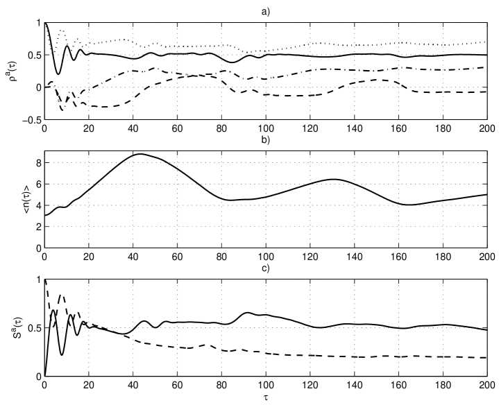
Figure 3: The same as in Fig.2 but for detuning $\delta=0.1$.

where $H_{i}$ is written in (2). For simplicity we only consider the case $\delta\neq 0$ and $\Delta=0$. Master equation (19) is more difficult to solve and numerical methods usually must be used. At interesting frequencies range the dissipation is written in Eq.(19) both as mirror losses in the cavity that defines the mode of the electromagnetic field $\mathcal{L}_{1}\rho$, and as spontaneous emission from the atom $\mathcal{L}_{2}\rho$. At Born-Markov approximation and zero temperature, these parts are written in equation (19) as the following. One term is as follows $\mathcal{L}_{1}\rho=\gamma_{1}\left(2a\rho a^{+}-a^{+}a\rho-\rho a^{+}a\right)$, where $\gamma_{1}$ is the rate of single-photon losses. Another term $\mathcal{L}_{2}\rho=\left(\gamma_{2}/2\right)\left(2\sigma\rho\sigma^{+}-\sigma^{+}\sigma\rho-\rho\sigma^{+}\sigma\right)$ takes into account the spontaneous emission from the atom out of the sides of the cavityO.Scully and Zubairy (1996). In this case the atom is damped by spontaneous emission with damping rate $\gamma_{2}$ to modes other than the privileged cavity mode with frequency $\omega_{a}$. We have solved the equation (19) numerically using a truncated number states $\left|n\right\rangle$ and atom states $\left|e\right\rangle$, $\left|g\right\rangle$ basis. The algorithms for integration of such a system numerically can be found, e.g. in Ref.H.Press et al. (2002). In general $0\leq n\leq\infty$, but for numerical calculations we have used $0\leq n\leq M$. A finite base of the number states $M$ was kept large enough so that the highest energy state is never populated significantly. Since we assume above that the field is initially in the coherent state $\left|\alpha\right\rangle$, and the atom is in the upper state $\left|e\right\rangle$, then initially $\rho=\left|\alpha\right\rangle\left\langle\alpha\right|\otimes\left|e\right\rangle\left\langle e\right|$ must hold. Using numerically obtained joint density matrix $\rho$  we have calculated the next quantities. Tracing out the matrix $\rho$ over the field (atom) states we have calculated the reduced atom (field) density matrix $\rho^{a,f}=Tr_{f,a}\{\rho\}$ , where $Tr_{a,f}\{\rho\}$ are the partial traces over the atom or field states accordingly. The latter allows us to study the dynamics of the excited-state probability $P^{+}(\tau)=\rho_{ee}^{a}$ , the mean photon number $\left\langle n(\tau)\right\rangle$ and the entropy $S^{a}(\tau)=-Tr\{\rho^{a}\ln\rho^{a}\}$. Also the Fourier spectrum of $P^{+}(\tau)$ is explored. The convergence of the equations is tested and the dynamics of the system is studied for different values of the external field relative to the atom-field mode coupling. The results of the numerical solution of master equation (19) are shown in Figs.1-4.

III Numerical results

We briefly consider the dynamics of a vacuum $\alpha=0$ of driving JCM in order to understand some general features first. Fig.1 shows the behavior of the atom quantities and mean photon number for resonant case ($\delta=0$) for vacuum initial state $\left|0\right\rangle$ at losses case, obtained as a result of the numerical solution of the master equation (19). This solution is close to Eq.(12), but with a damping due to both mirror losses in the cavity and spontaneous emission from the atom. We use the following parameters $\mathcal{E=}0.7$, $g=0.2$, $\gamma_{1}/\gamma_{2}=5$ and $\gamma_{1}=5\cdot 10^{-3}$. To make clearer the details of time evolution we use here a time interval $\tau=200$ , which is large in comparison with the characteristic time scale of revivalNarozhny et al. (1981) $\tau>2\tau_{R}$, where $\tau_{R}=2\gamma\pi/g$ $=55$, $\gamma=\mathcal{E}/2g=1.75$. One can see, that dynamics of the probability of excited level occupations $P^{+}(\tau)$ has form of a damped sequence of collapses and revivals. Dynamical collapses and revivals are specific features of a unitary evolution. They are strongly affected by decoherency, which have the time constant set by the cavity field energy damping time $\sim 1/(\gamma_{1}+\gamma_{2})$. From Fig.1(a) one can see that both collapses and revivals are progressively less pronounced due to dissipation $\gamma_{1,2}\neq 0$. The dissipation also reduces the magnitudes of non-diagonal elements $\rho_{ge}^{a}$ (in this case $\rho_{eg}^{a}=(\rho_{ge}^{a})^{\ast}$ are purely imaginary quantities). One can see, that quantity $\operatorname{Im}(\rho_{ge}^{a})$ over time approaches to zero due to losses, which causes the field phase information to wash out and progresses decoherence in the coupled system.

The dynamics $Tr\{(\rho^{a})^{2}\}$ in Fig.1(a)  shows that in the collapse area quantity $Tr\{(\rho^{a})^{2}\}$ has a maximum close to $1$ at $\tau_{0}=\tau_{R}/2=27.5$. This point corresponds to the atomic attractor state which is completely independent on the initial atomic stateGea-Banacloche (1990). At this point the compound system is in the disentangled state when in lossless system $S^{a,f}\rightarrow 0$ and $Tr\{(\rho^{a,f})^{2}\}\rightarrow 1$. In lossy system such limit values are fulfilled only approximately. One can see from Fig.1(b) that the mean photons number $\left\langle n\right\rangle$ increases from the initial zero value; however over time $\left\langle n\right\rangle$ assumes the steady-state value justified by the amplitude of external driving field $\mathcal{E}$. Fig.1(c) shows the dynamics of the entropy of atom subsystem $S^{a}(\tau)=-Tr\{\rho^{a}\ln\rho^{a}\}$. In the area of the first collapse $S^{a}$ has oscillating behavior. However these oscillations are smoothed away over time and $S^{a}(\tau)$ approaches to the steady-state value $ln(2)=0.69$, which corresponds to maximally entangled state of two-level atom and field mode. At a lossless case the exact equalities $Tr\{(\rho^{a})^{2}\}=Tr\{(\rho^{f})^{2}\}$ and $S^{a}=S^{f}$ in standard JCM hold Phoenix and Knight (1991). Our simulations confirm this fact with very good accuracy.

Next, we study details of the driving and initial coherent fields interaction. Fig.2(a) shows dynamics of the atom subsystem for the compensative case ($\widetilde{\gamma}=\gamma+\alpha=\mathcal{E}/2g+\alpha=0$) ( see Eq. (17) for the exact resonance case ($\delta=0$)), but taking into account dissipation $\gamma_{1,2}\neq 0$. Comparison of Fig.1(a) and Fig.2(a) shows that the dynamics for this case is essentially different from the that in the initial vacuum case $\alpha=0$ and has the form of damped vacuum Rabi oscillation in standard JCM.

Dynamics of the mean photons number $\left\langle n\right\rangle$ is of interest and is shown in Fig.2(b). The solid line in Fig.2(b) shows results $\left\langle n\right\rangle$ from a numerical simulation of the atom-field master equation (19) for the compensative case, taking into account losses in the system. For a short period of time $\tau<10$ this simulation is in very good agreement with the exact formula (18). However a discrepancy arises over time due to losses not included in (18). One can see that despite of the mutual compensation of the initial coherent field and driving field in Eq.(18), the mean number of photons oscillates in vicinity $\sim\left|\alpha\right|^{2}$, that is justified by the field $\left|\mathcal{E}\right|$. One can see from Fig.2(c), that for a short time the dynamics of entropy is similar to that in the vacuum case. However over longer time intervals the impact of dissipation becomes essential. Despite dissipation, at the time instances $\tau_{k}=\pi(2k+1)/2g$ , $k=0,1...$ the entropy $S^{a}(\tau_{k})$ is very close to zero that implies the transition of the coupled atom-field system to the uncoupled pure state. At the moments $\tau_{k}=\pi k/g$ the entropy has a value close to $\ln 2$, which corresponds to the maximum entanglement of the two-level atom and the field. Since the mean photon number does not vanish (see Fig.2(b)) this dynamics is stable asymptotically.

Fig.3 shows dynamics of the coupled subsystem in the compensative case ($\widetilde{\gamma}=0$) when both dissipation $\gamma_{1},\gamma_{2}\neq 0$ and detuning $\delta\neq 0$ are non-zero. Notice in a non-resonant case ($\delta\neq 0$) the time dependence in the Hamiltonian (2) is not removed, and therefore the displacement operators transformation already does not allow to reduce the driving JCM to standard JCM. Compared to the case of the exact resonance (Fig.2) the sequential collapses and revivals now practically disappear over long periods of time; in Fig.3(a) the first collapse is seen only. Nevertheless some maxima of $Tr\{(\rho^{a})^{2}\}$ remain resolvable. One can see from Fig.3(c) that during short periods of time $\tau<7$ the behavior $S^{a}$ is similar to a that in the vacuum case (Fig.2(c)). However over longer periods of time the influence of decoherence becomes essential. The entropy quickly approaches its asymptotic value.

Fig.4 shows the Fourier spectra for cases of driving JCM considered above. This spectrum, obtained by Fourier transform of numerically calculated $P^{+}(\tau)$, exhibits well separated discrete frequency components, which are scaled as square roots of the successive integers. The spectrum in Fig.4(a) corresponds to the time dynamics presented in Fig.1(a). One can see, that $P^{+}$ spectrum at the initial vacuum state $\left|0\right\rangle$ for driving JCM case is similar to that in a standard JCM (without driving field $\mathcal{E}=0$) at initial coherent field $\left|\alpha\right\rangle$. Note that for standard JCM such peaks were observed experimentally in Ref.Brune et al. (1996b). The spectrum in Fig.4 (a) is rather similar to the spectrum shown in Fig.2(d) of experimentBrune et al. (1996b) for $\gamma=1.77$. We can conclude that the vacuum case of driving JCM is similar to a standard JCM case with a coherent initial field, at least for the exact resonance. This conclusion reiterates the fact that coherent field state is as close to the classical field as quantum mechanics permitsGlauber (1963). Note that Fig.4(a) shows that peak number $2$ is the highest one. This also follows from the above mentioned. In this case $\widetilde{\gamma}=1.75$ therefore the calculated number of highest peak is $E[\widetilde{\gamma}^{2}-1]=2$.

Figs.4(b)-4(d) represent compensative case (17) for the loss and detuning case. Fig.4(b) shows the spectrum for case $\delta=0$, however for not small losses, which are. One can see only the peak, which corresponds to $n=0$ is present in the Rabi spectrum. Such spectrum in Fig.4 (b) corresponds to the measured spectrum shown in Fig.2 (a) in Ref.Brune et al. (1996b)  for nearly vacuum case (no injected fields). Thus, the conclusion about the possibility subtracting of the coherent and classical fields remains valid in the loss case also. In Fig.4(c) influence of detuning is shown for smaller losses. One can see, that even for $\delta=0.1$ which is not very small the spectrum of several first Rabi frequencies is well recognizable. There are a few peaks in Fig.4(c), which correspond to detuning $\delta\neq 0$. Such peaks are present even at a larger dissipation rate (the dissipation rate in Fig.4(d) are increased by two orders, with respect to Fig.4(c). Nevertheless the peak of vacuum oscillations remains dominant.

In general one can readily derive, that the quantity $\gamma$ can be rewritten (with the previously used notations) as $\gamma=\mathcal{E}/2g=E_{e}/E_{vac}$, where $E_{vac}=\left(\hbar\omega_{a}/2\varepsilon_{0}V\right)^{1/2}$ is the field per photon. Then from equality (17) $\widetilde{\gamma}=\gamma+\alpha=0$ one can obtain $E_{e}=E_{vac}\overline{n}^{1/2}\exp(i(v+\pi))$. The latter equation states that for the compensated case (17) the driving field $E_{e}$ should be in a coherent state, but shifted by phase $\pi$ concerning to initial state $\alpha$. In general, condition (17) does not hold exactly due to quantum fluctuations. However, since the ratio of fluctuation to the mean number (fractional uncertainty in the photon number, see e.g. Ch.3 in Ref.Gerry and Knight (2004)) is $\Delta n/\overline{n}=\overline{n}^{-1/2}$ for a Poisson process, the larger values of $\overline{n}$ become, the better is the accuracy of condition (17).

IV Conclusion

Studied the field-atom interactions in the driving JCM shows that a variation of the amplitude or/and the phase of the driving field enables one to manipulate the dynamics and the spectrum of quantum Rabi oscillations. There are two distinct regimes. In case of summation of the driving field and initial coherent field one can underscoring a selected frequency in the Rabi frequency spectrum. The subtraction provides a possibility of compensation of both fields. For the case of the exact compensation, the frequency spectrum of a two-level atom becomes similar to that of vacuum oscillations in standard JCM. To use these processes for quantum information technology, the decoherence time must be greater than the time scale of the atom-field interaction. In this case, these processes may have various applications related to monitoring of the entanglement of two-level atom with quantized field and may be used to develop quantum information technology devices.

V Acknowledgements

The author is grateful to Alexander (Sasha) Draganov (ITT Industries - Advanced Engineering & Science Division) who made several helpful comments.

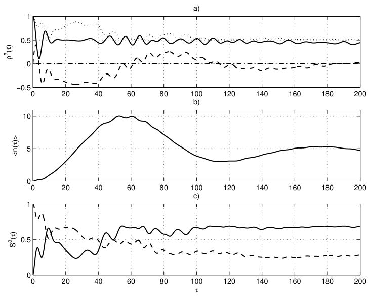
Figure 1: Quantum dynamics in driving JCM as function of the interaction time $\tau$ for initial vacuum case $\left|0\right\rangle$, $\delta=\Delta=0$, $\mathcal{E}=0.7$, $g=0.2$, $\gamma_{1}=5\cdot 10^{-3}$, $\gamma_{2}=10^{-3}$. (a) Probability of the excited level $\left|e\right\rangle$ occupations $P^{+}$ (solid line), $\operatorname{Im}(\rho_{ge}^{a})$ (dashed line), $Tr\{(\rho^{a})^{2}\}$ (dotted line). (b) Mean photon number $\left\langle n\right\rangle$. (c) Entropy $S^{a}$ (solid line), $Tr\{(\rho^{f})^{2}\}$ (dashed line). See details in text.

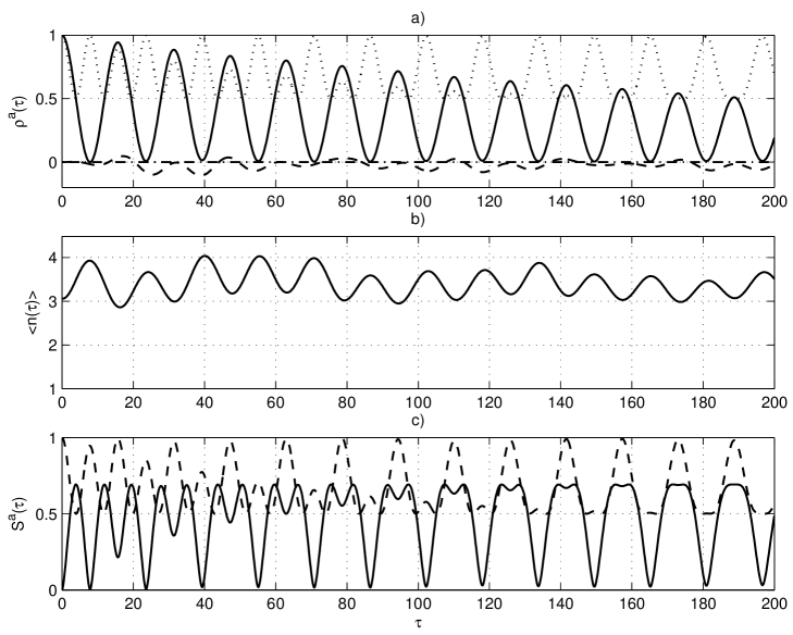
Figure 2: Quantum dynamics in driving JCM as function of the interaction time $\tau$ for initial coherent case $\left|\alpha\right\rangle$, $\alpha=-1.75$ (compensating case (17)), $\delta=\Delta=0$, $\mathcal{E}=0.7$, $g=0.2$, $\gamma_{1}=5\cdot 10^{-3}$, $\gamma_{2}=10^{-3}$. (a) Probability of the excited level $\left|e\right\rangle$ occupations $P^{+}$ (solid line), $\operatorname{Im}(\rho_{ge}^{a})$ (dashed line), $\operatorname{Re}(\rho_{ge}^{a})$ (dash-dot line), $Tr\{(\rho^{a})^{2}\}$ (dotted line). (b) Mean photon number $\left\langle n\right\rangle$. (c) Entropy $S^{a}$ (solid line), $Tr\{(\rho^{f})^{2}\}$ (dashed line). See details in text.

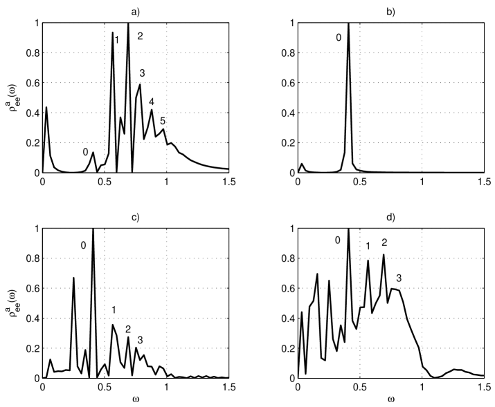
Figure 4: Fourier transforms of the probability $P^{+}(\tau)$ revealing the discrete Rabi frequencies, occurring at the successive square roots of the integers $\sqrt{n+1}$, numbers $n=0,1,2...$ are inserted in vicinity of peaks. Spectra correspond to (a) Fig.1(a); (b) Fig.2(a); (c) Fig.3(a), but with $\gamma_{1}=5\cdot 10^{-5}$, $\gamma_{2}=10^{-5}$; (d) Fig.3(a).

References

- Blinov et al. (2004) B. B. Blinov, D. L. Moehring, L.-M. Duan, and C. Monroe, Nature. 428, 153 (2004).
- Zurek (2003) W. H. Zurek, Rev. Mod. Phys. 75, 715 (2003).
- Raimond et al. (2001) J. M. Raimond, M. Brune, and S. Haroche, Rev. Mod. Phys. 73, 565 (2001).
- Brune et al. (1996a) M. Brune, E. Hagley, J. Dreyer, X. Maitre, A. Maali, C. Wunderlich, J. M. Raimond, and S. Haroche, Phys. Rev. Lett. 77, 4887 (1996a).
- Jaynes and Cummings (1963) E. Jaynes and F. Cummings, Proc. IEEE. 51, 89 (1963).
- Solano et al. (2003) E. Solano, G. S. Agarwal, and H. Walther, Phys. Rev. Lett. 90, 027903 (2003).
- Zheng (2002) S.-B. Zheng, Phys. Rev. A. 66, 060303 (4 pages) (2002).
- Zheng (2003) S.-B. Zheng, Phys. Rev. A. 68, 035801 (4 pages) (2003).
- Lougovski et al. (2004) P. Lougovski, F. Casagrande, A. Lulli, B.-G. Englert, E. Solano, and H. Walther, Phys. Rev. A. 69, 023812 (9 pages) (2004).
- Vahala (2003) K. J. Vahala, Nature. 424, 839 (2003).
- Artemyev et al. (2001) M. V. Artemyev, U. Woggon, and R. Wannemacher, Appl. Phys. Lett. 78, 1032 (2001).
- G.Burlak et al. (2003) G.Burlak, P. A. Marquez, and O.Starostenko, Phys. Lett. A. 309, 146 (2003).
- Alsing et al. (1992) P. Alsing, D.-S. Guo, and H. J. Carmichael, Phys. Rev. A. 45, 5135 (1992).
- Jyotsna and Agarwal (1993) I. V. Jyotsna and G. S. Agarwal, Opt. Commun. 99, 344 (1993).
- Dutra et al. (1993) S. M. Dutra, P. L. Knight, and H. Moya-Cessa, Phys. Rev. A. 48, 3168 (1993).
- Chough and Carmichael (1996) Y. T. Chough and H. J. Carmichael, Phys. Rev. A. 54, 1709 (1996).
- Gerry (2002) C. C. Gerry, Phys. Rev. A 65, 063801 (6 pages) (2002).
- Glauber (1963) R. Glauber, Phys. Rev. 131, 2766 (1963).
- J.-L.Basdevant and J.Dalibard (2002) J.-L.Basdevant and J.Dalibard, Quantum mechanics (Springer, 2002).
- Brune et al. (1996b) M. Brune, F. Schmidt-Kaler, A. Maali, J. Dreyer, E. Hagley, J. M. Raimond, and S. Haroche, Phys. Rev. Lett. 76, 1800 1803 (1996b).
- Yurke and Stoler (1986) B. Yurke and D. Stoler, Phys. Rev. Lett. 57, 13 (1986).
- Monroe et al. (1996) C. Monroe, D. M. Meekhof, B. E. King, and D. J. Wineland, Science. 272, 1131 (1996).
- O.Scully and Zubairy (1996) M. O.Scully and M. Zubairy, Quantum optics (Cambridge. University press, 1996).
- H.Press et al. (2002) W. H.Press, S. A.Teukovsky, W. T.Vetterling, and B. P.Flannery, Numerical recipes in C++ (Cambridge, University Press, Cambridge, 2002).
- Narozhny et al. (1981) N. B. Narozhny, J. J. Sanchez-Mondragon, and J. H. Eberly, Phys. Rev. A. 23, 236 (1981).
- Gea-Banacloche (1990) J. Gea-Banacloche, Phys. Rev. Lett. 65, 3385 (1990).
- Phoenix and Knight (1991) S. J. D. Phoenix and P. L. Knight, Phys. Rev. A. 44, 6023 (1991).
- Gerry and Knight (2004) C. Gerry and P. Knight, Introductory Quantum Optics (Cambridge University Press, 2004).