Dynamical phase transitions and temperature induced quantum correlations in an infinite spin chain

Abstract

We study the dynamics of entanglement in the infinite asymmetric $XY$ spin chain, in an applied transverse field. The system is prepared in a thermal equilibrium state (ground state at zero temperature) at the initial instant, and it starts evolving after the transverse field is completely turned off. We investigate the evolved state of the chain at a given fixed time, and show that the nearest neighbor entanglement in the chain exhibits a critical behavior (which we call a dynamical phase transition), controlled by the initial value of the transverse field. The character of the dynamical phase transition is qualitatively different for short and long evolution times. We also find a nonmonotonic behavior of entanglement with respect to the temperature of the initial equilibrium state. Interestingly, the region of the initial field for which we obtain a nonmonotonicity of entanglement (with respect to temperature) is directly related to the position and character of the dynamical phase transition in the model.

I Introduction

Exploring the properties of entanglement has recently attracted a lot of interest, due to the usefulness of entanglement in quantum information processing tasks NC . Recently, several authors have begun to study the properties of entanglement in real physical many body systems, such as cold atomic gases in optical lattices (e.g. optical_lattice ) or in trapped gaseous Bose-Einstein condensates (e.g. BEC ). It turns out that such investigations help us to understand the physics of quantum phase transitions (e.g. Osterloh ; Nielsen ; salikh-qwerty ; salikh-qwerty1 ; ent_length ). Moreover, they are important for implementations of quantum computation, or other quantum information processing tasks in such physical systems.

Among the potential candidates for implementing quantum computation are various models of spin systems that can be realised with ultracold atoms in optical lattices (see e.g. toolbox ; proposal_korechhey ). There is therefore a strong motivation behind the study of entanglement in spin systems (see e.g. Osterloh ; Nielsen ; salikh-qwerty ; salikh-qwerty1 ; ent_length ; Wootters ; Indranidi ; numerical ; amader ; Dagmar and references therein). Moreover, studies of entanglement in spin models help us to relate entanglement to the fundamental concepts, such as quantum phase transitions. In particular, it was shown that near a phase transition in the ground state of an exactly solvable spin model in one dimension (Ising model in a transverse field), two-particle entanglement remains short ranged, while two-particle correlation length diverges Osterloh ; Nielsen . The behavior of bipartite, as well as multipartite entanglement in the ground states and (thermal) equilibrium states of spin rings and chains has been studied from several perspectives Osterloh ; Nielsen ; salikh-qwerty ; Wootters ; amader ; Dagmar . It has been shown that, using the concept of localizable entanglement ent_length ; Ciracnew (cf. hmmmm ; amrao-achhi-re-bhai ), bounded from above by entanglement of assistance Bennett-assistance , and from below by correlation functions, one can define an entanglement correlation length that diverges at the criticality, and majorizes the standard correlation length (see also kachpoka ).

Studies of entanglement of the time-evolved state of spin models has also been carried out Briegel_orey_orey ; Sougato ; talk_dilo_Osterloh ; numerical ; amader ; meti-pukur . In particular, implementation of the “one-way quantum computer” and short range teleportation BBCJPW of an unknown state has been proposed by using the dynamics of spin systems in Briegel_orey_orey ; Briegel_ebong ; meti-pukur ; Sougato ; Sougato_ebong . In Ref. amader , it was shown that the nearest-neighbor entanglement of the time-evolved state in an infinite spin chain (asymmetric $XY$ model in a transverse field), after an initial disturbance, does not approach its equilibrium value (nonergodicity of entanglement). Previous studies of quantum dynamics of spin models after a rapid change of the field include Refs. Stephenexpt ; Stephen , while effects of a sudden switching of the interaction in arrays of oscillators were studied in Ref. Martin .

In this paper, we study the dynamics of nearest-neighbor entanglement in the evolution of an infinite spin chain described by the asymmetric $XY$ model in a transverse field (see Eq. (2) below). We take the initial state of the evolution to be the equilibrium state at zero temperature, and suddenly turn off the transverse field at zero time. The system is thus given an initial disturbance, and its properties are then studied at later times. We find that the nearest-neighbor entanglement in the evolved state at a fixed time shows a criticality (which we call a dynamical phase transition (DPT)) with respect to the transverse external field. We refer to the region of the initial transverse field for which the entanglement is nonvanishing (vanishing), at a fixed time, as the “entangled phase” (“separable phase”). Interestingly, the nature of the DPT depends on whether we are near, or far from the time of initial disturbance. Moreover, for values of the initial transverse field near the criticalities, as well as in the separable phase, and for short times, the nearest-neighbor entanglement shows nonmonotonicity with respect to temperature. Accordingly, we call the criticalities as “critical regions”, signifying that “critical” effects persist for a small region around the critical value of the transverse field. Such nonmonotonicity of entanglement with respect to temperature was also found in Ref. Scheel , in the Jaynes-Cummings model. Study of nonmonotonicity of entanglement with respect to temperature is interesting, as preservation of entanglement in a hostile environment is one of the main challenges in quantum computation and quantum information in general. A common belief is that temperature is a form of noise, i.e. it destroys the subtle quantum correlations. However, we show that for the infinite spin chain modelled by the $XY$ Hamiltonian, at least in some situations, entanglement is not always monotonically decreasing with temperature, and interestingly, this is related to the appearance of a dynamical phase transition in that model.

As we have mentioned above, we characterise the DPT in the asymmetric $XY$ chain by magnetic field and temperature, the usual control parameters used in statistical physics for characterising phase transitions. However, note that we also use time ($t$) as one of our control parameters in the characterisation. As we will see in this paper, significant change of behavior is observed in the DPTs, as we change the parameter $t$.

The paper is organised as follows. In Sec. II, we will recollect some facts about the $XY$ spin model and fix some notations. In order to explore the properties of entanglement, one has to fix the measure with which one quantifies entanglement. In Sec. III, we define the entanglement measure that will be considered in this paper. The concept of dynamical phase transition is discussed in Sec. IV. The nonmonotonicity of entanglement of the evolved state with respect to temperature of the initial state, and its connection to the dynamical phase transition, are discussed in Sec. V. We summarize our results in the final section (Sec. VI).

II The $XY$ model in the transverse field

II.1 Description of the model

For a one-dimensional spin chain of spin 1/2 particles, a simple form of the Hamiltonian with nearest neighbor interactions is given by

$$H_{int}=\sum_{i}({\cal A}S_{i}^{x}S_{i+1}^{x}+{\cal B}S_{i}^{y}S_{i+1}^{y}+{\cal C}S_{i}^{z}S_{i+1}^{z}),$$ (1)

where $A$, $B$, and $C$ are coupling constants, and $S_{i}^{x}$, $S_{i}^{y}$, $S_{i}^{z}$ are spin 1/2 operators (one-half of the Pauli matrices) at the $i$-th site. One can also introduce an external magnetic field in the Hamiltonian, so that the total Hamiltonian is

$$H=H_{int}-h(t)H_{mag},$$

where $h(t)$ is a time-dependent function, to be specified below. To obtain a non-trivial effect on the dynamics due to the field part of the Hamiltonian, one must choose the magnetic field and other parameters in such a way that the interaction part and the field part of the total Hamiltonian do not commute.

A simple way to attain that is to choose the field part as

$$H_{mag}=\sum_{i}S_{i}^{z},$$

and $A=1+\gamma$, $B=1-\gamma$, $C=0$ (with $\gamma\neq 0$). Therefore the total Hamiltonian that we study in this paper takes the form ($\gamma\neq 0$)

$$H=\sum_{i}\left((1+\gamma)S_{i}^{x}S_{i+1}^{x}+(1-\gamma)S_{i}^{y}S_{i+1}^{y}\right)-h(t)\sum_{i}S_{i}^{z}.$$ (2)

This Hamiltonian is called the asymmetric $XY$ model in a transverse field.

Such a system can be realized in atomic gas in an optical lattice (e.g. toolbox ; proposal_korechhey ). Note that the condition of nonvanishing anisotropy $\gamma$ is required, as otherwise the field part commutes with the interaction part. This model is exactly solvable by succesive Jordan-Wigner, Fourier, and Bogoliubov transformations LSM . We still have to specify the time dependence of the magnetic field, which we choose to be a step function. Precisely, we choose $h(t)$ to be

$$h(t)=\Big{\{}\begin{array}[]{c}a,\quad t\leq 0\\ 0,\quad t>0\end{array},$$

with $a\neq 0$. The system is thus given an initial disturbance, as the field is turned off. The properties of the evolved state are then studied at later times.

We will mainly be interested in studying the dynamics of nearest neighbor entanglement of the evolved state of such model. The state that we consider, evolves according to the Hamiltonian $H$, given in Eq. (2). But it also depends on the initial state, from which it starts evolving. Let us denote the (thermal) equilibrium state at the initial time, and at absolute temperature $T$ as $\rho_{\beta}^{eq}$:

$$\rho_{\beta}^{eq}=\mbox{exp}[-\beta H(0)]/Z_{\beta}.$$

Here $Z_{\beta}$ is the partition function, given by

$$Z_{\beta}={\rm tr}(\mbox{exp}[-\beta H(0)]),$$

and $\beta=\frac{1}{kT}$, where $k$ is the Boltzmann constant. Henceforth, we set $k=1$. In all cases studied here, we will be choosing an equilibrium state $\rho^{eq}_{\beta}$ as our initial state. In particular, we will consider the case of zero temperature, i.e. when $\beta\rightarrow\infty$.

II.2 Single and two particle reduced density matrices

Although our main intention is to study the behavior of nearest neighbor entanglement, we will also calculate the single-site property of magnetization in this model. As we will see, the behavior of magnetization (in particular, its nonmonotonicity) does not depend on whether we are near, or far from the DPT discussed in this paper. Let us therefore find out the single-site and two-site reduced density matrices of the evolved state. Let us suppose that the evolution starts off from the initial state $\rho^{eq}_{\beta}$ of the infinite chain, and let the evolved state of the infinite spin chain be denoted by $\rho_{\beta}(t)$. Due to symmetry, all the single-site density matrices of the evolved state (at a particular instant $t$, and for a particular temperature $T$) are equal. The same is true for the nearest neighbor density matrices (as for the other two-site density matrices). We denote them as $\rho^{1}_{\beta}(t)$ and $\rho^{12}_{\beta}(t)$, respectively.

Our system is an infinite spin chain of spin-1/2 particles, and so our single-site density matrix $\rho^{1}_{\beta}(t)$ acts on the two-dimensional complex Hilbert space. A general single qubit (two-dimensional quantum system) density matrix can be written as

$$\rho^{1}_{\beta}(t)=\frac{1}{2}I+2M^{z}_{\beta}(t)S^{z}+2M^{x}_{\beta}(t)S^{x}+2M^{y}_{\beta}(t)S^{y},$$

where $M^{z}_{\beta}(t)$, $M^{x}_{\beta}(t)$, $M^{y}_{\beta}(t)$ are the unknown parameters to be determined. Using Wick’s theorem, as in Refs. LSM ; McCoy1 ; McCoy_eka , we have that

$$M^{x}_{\beta}(t)=M^{y}_{\beta}(t)=0.$$ (3)

Therefore the single-site density matrix of the evolved state is of the form

$$\rho^{1}_{\beta}(t)=\frac{1}{2}I+2M^{z}_{\beta}(t)S^{z},$$

so that we are left with determining just the single parameter

$$M^{z}_{\beta}(t)={\rm tr}\left(S^{z}\rho^{1}_{\beta}(t)\right),$$

which is the (transverse) magnetization of the system.

Let us now consider the two-site density matrix $\rho_{\beta}^{12}$ of the evolved state. A general two-qubit state is of the form

$$\rho^{12}_{\beta}(t) = \frac{1}{4}I\otimes I+\sum_{j=x,y,z}M^{j}_{\beta}(t)(S^{j}\otimes I+I\otimes S^{j})$$ (4)

$$+ \sum_{j,k=x,y,z}T^{jk}_{\beta}(t)S^{j}\otimes S^{k},$$

where

$$T^{jk}_{\beta}(t)=4{\rm tr}\left(S^{j}\otimes S^{k}\rho^{12}_{\beta}(t)\right)$$

are the two-site correlation functions. We already have $M^{x}_{\beta}(t)=M^{y}_{\beta}(t)=0$. By applying Wick’s theorem again, one can find that the $x-z$ and the $y-z$ correlations are vanishing. Therefore, the two-site density matrix of the evolved state is of the form

$$\rho^{12}_{\beta}(t) = \frac{1}{4}I\otimes I+M^{z}_{\beta}(t)(S^{z}\otimes I+I\otimes S^{j})$$ (5)

$$+ T^{xy}_{\beta}(t)(S^{x}\otimes S^{y}+S^{y}\otimes S^{x})$$

$$+ \sum_{j=x,y,z}T^{jj}_{\beta}(t)S^{j}\otimes S^{j}.$$

To find out the remaining (nonvanishing) parameters of the single and two particle states ($\rho^{1}_{\beta}(t)$ and $\rho^{12}_{\beta}(t)$ respectively), explicit use of diagonalizing transformations (Jordan-Wigner, Fourier, and Bogoliubov transformations) must be made LSM ; McCoy1 ; McCoy_eka . Using them, one finds that the (transverse) magnetization of the evolved state is given by McCoy1

$$M^{z}_{\beta}(t) = \frac{1}{2\pi}\int_{0}^{\pi}d\phi\frac{\mbox{tanh}(\frac{1}{2}\beta\Lambda(a))}{\Lambda(a)\Lambda^{2}(0)}$$

$$\times \Big{\{}\left[\cos(2\Lambda(0)t)\gamma^{2}a\sin^{2}\phi\right]$$

$$- \cos\phi\left[(\cos\phi-a)\cos\phi+\gamma^{2}\sin^{2}\phi\right]\Big{\}},$$

where $\Lambda(a)$ and $\Lambda(0)$ are obtained from $\Lambda(h(t))=[\gamma^{2}\sin^{2}\phi+(h(t)-\cos\phi)^{2}]^{\frac{1}{2}}$. The nearest neighbor correlations of the evolved state are given by McCoy_eka $T^{xy}_{\beta}(t)=S_{\beta}(1,t)/i$, $T^{xx}_{\beta}(t)=-G_{\beta}(-1,t)$, $T^{yy}_{\beta}(t)=-G_{\beta}(1,t)$, $T^{zz}_{\beta}(t)=4[M^{z}_{\beta}(t)]^{2}-G_{\beta}(1,t)G_{\beta}(-1,t)+S_{\beta}(1,t)S_{\beta}(-1,t)$, where $G_{\beta}(R,t)$ and $S_{\beta}(R,t)$, for $R=\pm 1$, are given by

$$G_{\beta}(R,t) = \frac{\gamma}{\pi}\int_{0}^{\pi}d\phi\sin(\phi R)\sin\phi\frac{\mbox{tanh}\left(\frac{1}{2}\beta\Lambda(a)\right)}{\Lambda(a)\Lambda^{2}(0)}$$

$$\times\big{[}\gamma^{2}\sin^{2}\phi + (\cos\phi-a)\cos\phi$$

$$\quad\quad\quad\quad+a\cos\phi\cos(2\Lambda(0)t)\big{]}$$

$$- \frac{1}{\pi}\int_{0}^{\pi}d\phi\cos(\phi R)\frac{\mbox{tanh}\left(\frac{1}{2}\beta\Lambda(a)\right)}{\Lambda(a)\Lambda^{2}(0)}$$

$$\times\big{[}\{\gamma^{2}\sin^{2}\phi + (\cos\phi-a)\cos\phi\}\cos\phi$$ (7)

$$\quad\quad-a\gamma^{2}\sin^{2}\phi\cos(2\Lambda(0)t)\big{]},$$

$$S_{\beta}(R,t) = \frac{\gamma ai}{\pi}\int_{0}^{\pi}d\phi\sin(\phi R)\sin\phi\frac{\sin\left(2t\Lambda(0)\right)}{\Lambda(a)\Lambda(0)}.$$

III Measure of entanglement: Logarithmic negativity

Let us now specify the measure of entanglement, which we will use to quantify entanglement of the nearest neighbor spins of our infinite spin chain. There are several ways to quantify entanglement (see e.g. MichalQIC ; Bennett-assistance ), and in fact there exists no “canonical” entanglement measure. In this paper, we will consider logarithmic negativity (LN) VidalWerner . It should be stressed, however, that the results do not depend on the choice of the entanglement measure. To define logarithmic neagativity, let us first introduce negativity. The negativity $N(\rho_{AB})$ of a bipartite state $\rho_{AB}$ is defined as the absolute value of the sum of the negative eigenvalues of $\rho_{AB}^{T_{A}}$, where $\rho_{AB}^{T_{A}}$ denotes the partial transpose of $\rho_{AB}$ with respect to the $A$-part Peres_Horodecki . The logarithmic negativity is defined as

$$E_{N}(\rho_{AB})=\log_{2}(2N(\rho_{AB})+1).$$

In our case, the bipartite states are states of two qubits, so that $\rho_{AB}^{T_{A}}$ has at most one negative eigenvalue Anna-ek . Moreover, for two-qubit states, a positive LN implies that the state is entangled and distillable Peres_Horodecki ; Horodecki_distillable , while $E_{N}=0$ implies that the state is separable Peres_Horodecki .

IV Dynamical phase transition of the $XY$ spin chain

In this section, we consider the nearest neighbor entanglement of the evolved state in the $XY$ model of the infinite spin chain, at a fixed time $t$. We assume that the initial state is a state of thermal equilibrium at zero temperature, in the presence of the transverse field. We find that the nearest neighbor entanglement shows a critical behavior, which we call a dynamical phase transition. Precisely, the nearest neighbor logarithmic negativity of the evolved state, when considered at a given time, shows a criticality as a function of the initial transverse field. Moreover, the character of this dynamical phase transition depends on whether we are near or far from the initial time of disturbance. The observed phase transition is generic, as it occurs for a wide range of the anisotropy $\gamma$.

Note here that the evolved state at the time $t$ may be considered as a stationary state of the system, provided the dynamics is turned off after time $t$, i.e. the Hamiltonian (2) is set to zero at time $t$. We stress that turning off the Hamiltonian at time $t$ is experimentally feasible toolbox ; proposal_korechhey .

Let us first consider the behavior of the nearest neighbor entanglement with respect to the initial transverse field $a$, at a time $t$ that is near the initial time of disturbance. In Fig. 1, we plot the nearest neighbor LN of the evolved state with respect to $a$, at $t=1$, and for the anisotropy $\gamma=0.5$.

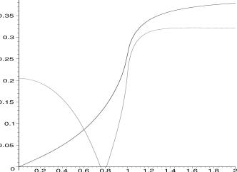
Figure 1: The nearest neighbor logarithmic negativity ($E_{N}$) of the evolved state, plotted as a function of the initial transverse field $a$, at a time that is near the time of initial disturbance ($t=1$). We fix the anistropy at $\gamma=0.5$. The initial state of evolution is a state of thermal equilibrium at zero temperature. $E_{N}$ vanishes at a critical value $a_{c}$ and revives at $\overline{a}_{c}$. We will show in Sec. V that for values of the initial field in the region near the phase transitions, entanglement behaves nonmonotonically with respect to the temperature of the initial equilibrium state. The transverse magnetization ($M^{z}$) of the evolved state is also plotted; it does not show a similar critical behavior as a function of $a$.

Entanglement exhibits criticalities, as the system parameter $a$, i.e. the initial transverse field is changed: $E_{N}$ vanishes at a critical value $a_{c}$ and revives at another critical value $\overline{a}_{c}$. Note that a similar phenomenon is absent for magnetization. We will see in the succeeding section that for values of the initial field that is close to the critical regions, entanglement of the evolved state behaves nonmonotonically as a function of the temperature of the initial equilibrium state.

Similar DPT’s of entanglement, as the system parameter $a$ changes, can be seen for other values of the time $t$, sufficiently near to the initial moment of disturbance, as well as for other values of the anisotropy $\gamma$.

However, as the time grows, the nature of the DPT changes significantly. In Fig. 2, we plot the nearest neighbor LN for a time that is comparatively far away from $t=0$, against the initial field $a$.

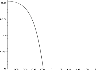
Figure 2: The nearest neighbor logarithmic negativity ($E_{N}$) of the evolved state $\rho^{12}_{\beta}(t)$ is plotted against the initial transverse field $a$, at $t=10$, which is comparatively large, as compared to that of Fig. 1. We again fix the anistropy $\gamma=0.5$, and $\beta\rightarrow\infty$, as in Fig. 1. Here we observe again a kind of criticality, but of a significantly different character than the one in Fig. 1. In Section V, we show that entanglement behaves monotonically as a function of temperature of the initial equilibrium state, for $a\approx a_{c}$ in this regime of $t$’s.

Again, a dynamical phase transition is observed, but one that is different from the one observed in Fig. 1. In Fig. 2, the system undergoes a phase transition from the entangled phase to the separable phase at $a_{c}$, but no re-entrance behavior is observed. Moreover, in the suceeding section, we show that the nonmonotonicity of entanglement is no longer present in this case of large $t$. A signature of dynamical phase transition is absent for magnetization for both small and large $t$.

To obtain a global perspective of the behavior of entanglement, we plot it with respect to both $t$ and $a$, at a fixed value of the anisotropy $\gamma$ ($\gamma=0.5$) in Fig. 3.

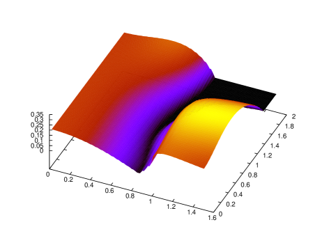
Figure 3: The nearest neighbor logarithmic negativity ($E_{N}$) of the evolved state $\rho^{12}_{\beta\rightarrow\infty}(t)$ is plotted against the initial transverse field $a$ and time $t$ for the anisotropy $\gamma=0.5$. On the $E_{N}=0$ plane, there are two curves of DPTs, both of which start at around $\{a=0.8,t=0\}$, and then they diverge off with increasing $t$, forming a “river” of separable states between themselves. The $t=1$ and $t=10$ slices of this surface were already discussed before. For the $t=0$ slice, entanglement is seen to vanish, as it should, as $a$ grows. Note that this is different from the $t=1$ slice behavior, where the entanglement converges to a positive value.

Note that a similar behavior is absent in magnetization, as seen in Fig. 4.

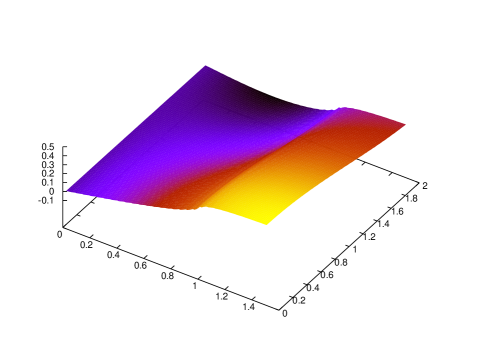
Figure 4: The magnetization ($M^{z}$) of the evolved state $\rho^{12}_{\beta\rightarrow\infty}(t)$ is plotted against the initial transverse field $a$ and time $t$ for the anisotropy $\gamma=0.5$.

An interpretation of the results for small and large $a$ (as compared to the region of phase transitions) is the following: For small $a$, the initial state is entangled, and its entanglement survives even for long times $t$ (see Fig. 2). On the other hand, for large $a$, the initial state is close to a separable state. This state is however, very different from any eigenstate of the Hamiltonian, and is thus very strongly affected by the dynamics, generating significant entanglement for small times $t$. The case of large $a$ is therefore similar to that in Refs. Briegel_orey_orey ; Briegel_ebong , where the time-independent Ising Hamiltonian with interaction in the $z$-direction, is made to act on a product of eigenstates of $\sigma_{x}$.

Note here that in contrast to the case of small $a$, there is no revival of entanglement with respect to time $t$, for large $a$ and large $t$ (compare Fig. 1 and Fig. 2). This feature is different from that in the Ising Hamiltonian, or from that in spin glass rotating-vase , where the state re-enters to the entangled and separable phases again and again after certain time intervals. The continuous character of the spectrum of the infinite $XY$ chain is most probably responsible for this effect: The dynamics is mixing the states in such a way that for large $a$, the revival of entanglement is possible only for relatively short times $t$, or alternatively, that for large $t$, there is no entanglement at large $a$.

V Nonmonotonicity of entanglement with temperature

In the preceding section, we have obtained the DPT of nearest neighbor entanglement of the evolved state of the infinite spin chain. The DPT was controlled by the transverse field $a$. The initial state of the evolution, however, was taken to be the equilibrium state at zero temperature. In this section, we will study this criticality and the monotonicity of nearest neighbor entanglement, considered as a function of the temperature of the initial equilibrium state.

For definiteness, consider the dynamical phase transition of Fig. 1, observed for the nearest neighbor entanglement of the evolved state at time $t=1$, and for the anisotropy $\gamma=0.5$. The evolution there had started from the equilibrium state at zero temperature. Consider now the evolution in which the initial state is the equilibrium state $\rho^{eq}_{\beta}$, at a certain temperature $T=1/\beta$. We again look at the nearest neighbor entanglement of the evolved state at time $t=1$ and for anisotropy $\gamma=0.5$, but now as a function of the temperature $T$ of the initial equilibrium state, and for a given value of the initial transverse field. It turns out that the behavior of entanglement (with respect to temperature) is qualitatively different, depending on whether we are near or far away from the dynamical phase transition of entanglement in Fig. 1. We find that it is possible to obtain three qualitatively different regions of the transverse field $a$, according to the behavior of entanglement with respect to the temperature of the initial equilibrium state.

1. The initial transverse field $a$ is far away (either lower or higher) from the critical regions: In this case, the nearest neighbor LN is monotonic with respect to the temperature of the initial equilibrium state. As temperature is lowered, LN increases monotonically, and ultimately converges to a nonzero value. This is illustrated in Fig. 5, for an exemplary value of $a=0.5$, that is comparatively far away from the critical region (in comparison to the cases considered in item (iii)).

   

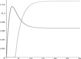
   Figure 5: The logarithmic negativity $E_{N}$ of the state $\rho^{12}_{\beta}(t)$, is plotted as a function of the inverse temperature $\beta$ of the initial equilibrium state $\rho^{eq}_{\beta}$. We choose $t=1$ and $\gamma=0.5$, just as in Fig. 1. The transverse field $a$ is chosen to be $0.5$, which is supposed to be comparatively far away from the critical regions in Fig. 1 (in comparison to the values of $a$ used in Figs. 7 and 8 below). We find that entanglement increases monotonically with decreasing $T$ (increasing with $\beta$). For reference and comparison, we also plot the transverse magnetization $M^{z}$ of $\rho_{\beta}(t)$.

2. The initial field is within the separable phase: The nearest neighbor LN is nonmonotonic with respect to the temperature of the initial equilibrium state. In particular, there are regions of temperature for which entanglement increases with increasing temperature (see also Ref. Scheel in this respect). A plot of nearest neighbor LN with respect to the initial temperature, is given in Fig. 6, for an exemplary value of the transverse field in the separable phase.

   

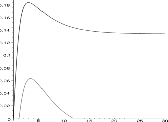
   Figure 6: The logarithmic negativity $E_{N}$ of the state $\rho^{12}_{\beta}(t)$, is plotted as a function of the inverse temperature $\beta$ of the initial equilibrium state $\rho^{eq}_{\beta}$. We choose $t=1$ and $\gamma=0.5$, just as in Fig. 1. The transverse field $a$ is chosen to be $0.78$, which is within the separable phase in Fig. 1. We find that entanglement is nonmonotonic with respect to temperature. In particular, therefore, there is range of temperature, for which entanglement is increasing with increasing temperature. For sufficiently low $T$ (and, as expected, for high $T$), entanglement is vanishing, in contrast to the situation in Figs. 7 and 8 below. Again, for reference and comparison, we also plot the transverse magnetization $M^{z}$ of $\rho_{\beta}(t)$.

   Note that entanglement in this case is nonvanishing only for moderate values of $T$. For very high and very low $T$, entanglement vanishes. This is different than in item (iii) below.

3. The initial field is in the critical region of the entangled phase: If the transverse field is sufficiently close to the critical region, but still being in the entangled phase, the nearest neighbor LN is again nonmonotonic with respect to the temperature of the initial state. However, the added feature is that the entanglement converges to a nonvanishing value for low $T$. In case (ii), the entanglement is vanishing for sufficiently low $T$ (and hence for sufficiently large $\beta$) (see Fig. 6). For sufficiently high $T$, entanglement is of course again vanishing, just as in the items (i) and (ii) above. The nearest neighbor LN, plotted for two exemplary values of $a$ in the region under consideration, are given in Figs. 7 and 8.

   

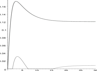
   Figure 7: The logarithmic negativity $E_{N}$ of the state $\rho^{12}_{\beta}(t)$, is plotted as a function of the inverse temperature $\beta$ of the initial equilibrium state $\rho^{eq}_{\beta}$. We choose $t=1$ and $\gamma=0.5$, just as in Fig. 1. The transverse field $a$ is chosen to be $0.74$, which is in a critical region in Fig. 1, but in the entangled phase (the first entangled phase). Just as in Fig. 6, we find that entanglement is nonmonotonic with respect to temperature. However, in contrast to the case in Fig. 6, entanglement is nonvanishing for low $T$. For sufficiently low $T$, entanglement converges to a nonvanishing value. For comparison, we also plot the transverse magnetization $M^{z}$ of $\rho_{\beta}(t)$.

   

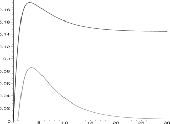
   Figure 8: The logarithmic negativity $E_{N}$ and the transverse magnetization $M_{z}$ of the state $\rho^{12}_{\beta}(t)$, are plotted as functions of the inverse temperature $\beta$ of the initial equilibrium state $\rho^{eq}_{\beta}$. We choose $t=1$ and $\gamma=0.5$, just as in Fig. 1. The transverse field $a$ is chosen to be $0.81$, which is again (just as in Fig. 7) in a critical region of Fig. 1, but in the entangled phase (the second entangled phase). The qualitative features of $E_{N}$ are just as in Fig. 7 above.

We stress that although we have considered here the case only for $\gamma=0.5$, the results are generic and have been numerically checked for several values of $\gamma$.

It is to be noted that the behavior of transverse magnetization does not seem to alter considerably as we pass from one entangled phase to another, through the separable phase, as is seen in Figs. 5, 6, 7, 8. The absence of this feature in magnetization, and its presence in entanglement, once again underlines that complexity of physical phenomena can be understood in terms of entanglement.

With respect to the nonmonotonicity of entanglement with the temperature of the initial state, let us note here that the usual intuition is that entanglement is a fragile quantity, and therefore it decays with noise. It is also usual to see an increase of temperature as a model of increase of noise in the system. This is for instance corroborated here in Figs. 5, 6, 7, 8, where entanglement vanishes for sufficiently large temperatures. However, we see here that for moderate values of $T$, the fragility of entanglement is a more complex issue. There can be ranges of temperatures for which entanglement actually increases with temperature.

Until now, we have been discussing the temperature effects for the dynamical phase transitions that were exemplified in Fig. 1 of the preceding section. A different sort of DPT was also obtained in the preceding section, as exemplified in Fig. 2. Surprisingly, in this case, the nearest neighbor entanglement does not behave as in the case of Fig. 1.

In Fig. 2, we plotted the nearest neighbor LN of the evolved state at time $t=10$, which is comparatively far away from the point of initial disturbance in the transverse field. The plot was with respect to the system parameter $a$, and a criticality was obtained at $a\approx 0.8$, for the anisotropy $\gamma=0.5$. We consider now the nearest neighbor entanglement of the evolved state at the time $t=10$ and for $\gamma=0.5$, as a function of the temperature of the initial equilibrium state. As we see, in contrast to the case of the phase transitions in Fig. 1, the nearest neighbor entanglement does not change its behavior as we choose different values of the transverse field $a$. In particular, the nearest neighbor LN of the evolved state is monotonic with temperature, and converges to a nonvanishing value for low $T$ (large $\beta$). In Fig. 9, we plot the nearest neighbor LN with respect to the initial temperature, for $a=0.8$, $t=10$, $\gamma=0.5$.

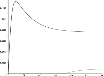
Figure 9: The logarithmic negativity $E_{N}$ of the state $\rho^{12}_{\beta}(t)$, is plotted as a function of the inverse temperature $\beta$ of the initial equilibrium state $\rho^{eq}_{\beta}$. We choose $t=10$ and $\gamma=0.5$, just as in Fig. 2. The transverse field $a$ is chosen to be $0.8$, which is approximately just the point of phase transition in Fig. 2. Although we are almost on the point of phase transition, we find that in contrast to the case of near-time phase trasnition, entanglement is monotonic with respect to temperature. For comparison, we also plot the transverse magnetization $M^{z}$ of $\rho_{\beta}(t)$.

However this feature is generic. We have also obtained similar features for several values of $\gamma$.

In Ref. ent_length , the authors define an entanglement length (range of quantum correlations), which is shown to diverge at the critical points for a wide range of spin systems. The definition is in terms of a quantity called localizable entanglement, which is usually hard to compute. However, there is a useful upper bound of this quantity in terms of the entanglement of assistance Bennett-assistance . Considering this upper bound for the case of the nearest neighbor density matrix, as well as for the next-nearest neighbor density matrix, we have checked that such definition of entanglement length does not seem to be able to characterise the dynamical phase transitions discussed in this paper. This indicates that the quantum phase transitions considered in Ref. ent_length are of a different character from the ones discussed here. Moreover, the behavior of entanglement with temperature of the system, can be seen as an independent candidate for understanding the phase transitions in the system.

VI Discussion

In this paper, we have investigated the dynamics of entanglement in the evolution of the infinite asymmetric $XY$ spin chain, in an initial transverse field. One motivation behind our study is that the dynamics of entanglement in the evolution of many-body spin-systems have been used to implement quantum computation and short range quantum communication Briegel_orey_orey ; Sougato . We also hope to be able to understand the physical phenomena in complex systems with the help of entanglement Osterloh ; Nielsen ; ent_length ; numerical .

For short times, we found a critical behavior of nearest neighbor entanglement of the system, with respect to the initial transverse field. The nearest neighbor entanglement vanishes for a certain value of the initial transverse field, to enter into the separable phase from an entangled phase. For a higher value of the field, there is a revival of entanglement, and the system re-enters into the entangled phase. For long times, there is again a criticality as the system moves from an entangled phase to a separable phase. However, there is no re-entrance into the entangled phase. In both cases studied, the system evolved from an initial (thermal) equilibrium state at zero temperature, and then we consider the nearest neighbor entanglement of the system at a fixed time. We refer to the regions of the transverse field, where the transition from entangled phases to separable phases occur, as the critical regions.

Surprisingly, we have shown that the nearest neighbor entanglement is nonmonotonic with respect to temperature in these critical regions, for short times. Similar behavior can also be seen in the separable phase. However for values of the transverse field that is deep inside the entangled phases, entanglement is strictly decreasing with temperature, both for short and long times.

Finally, let us note that it is important to consider the behavior of entanglement with respect to temperature in many body systems, as one of the main challenges in implementing quantum information processing tasks is to preserve entanglement in a noisy environment. Temperature is a usual intuitive way to model noise in such systems. Our findings indicate that the behavior of entanglement with respect to temperature, at least for moderate values of temperature, is quite complex. In particular, we found that for some ranges of temperature, entanglement in the system can grow with increasing temperature. It is interesting to look for similar nonmonotonic behavior of entanglement with respect to noise in the system, in other physical models, to find out how general such behavior can be.

- (1) M.A. Nielsen and I.L. Chuang, Quantum Computation and Quantum Information (Cambridge University Press, Cambridge, 2000).
- (2) For the theory, see e.g. D. Jaksch, C. Bruder, J.I. Cirac, C.W. Gardiner, and P. Zoller, Phys. Rev. Lett. 81, 3108 (1998); D. Jaksch, H.-J. Briegel, J.I. Cirac, C.W. Gardiner, and P. Zoller, Phys. Rev. Lett. 82, 1975 (1999); J.K. Pachos and M.B. Plenio, Phys. Rev. Lett. 93, 056402 (2004); C. Moura Alves and D. Jaksch, Phys. Rev. Lett. 93, 110501 (2004). For the experiments, see e.g. O. Mandel, M. Greiner, A. Widera, T. Rom, T.W. Hänsch and I. Bloch, Nature 425, 937 (2003).
- (3) L.-M. Duan, A. Sørensen, J.I. Cirac, and P. Zoller, Phys. Rev. Lett. 85, 3991 (2000); M.G. Moore and P. Meystre, Phys. Rev. Lett. 85, 5026 (2000).
- (4) A. Osterloh, L. Amico, G. Falci, and R. Fazio, Nature 416, 608 (2002).
- (5) T. Osborne and M.A. Nielsen, Phys. Rev. A 66, 032110 (2002).
- (6) G. Vidal, J.I. Latorre, E. Rico, and A. Kitaev, Phys. Rev. Lett. 90, 227902 (2003); J.I. Latorre, E. Rico, and G. Vidal, QIC 4, 48 (2004).
- (7) J. Vidal, R. Mosseri, and J. Dukelsky, Phys. Rev. A 69, 054101 (2004); L.-A. Wu, M. S. Sarandy, and D. A. Lidar, Phys. Rev. Lett. 93, 250404 (2004); M.-F. Yang, Phys. Rev. A 71, 030302 (R) (2005).
- (8) F. Verstraete, M. Popp, and J.I. Cirac, Phys. Rev. Lett. 92, 027901 (2004); F. Verstraete, M.A. Martin-Delgado, and J.I. Cirac, ibid., 087201 (2004).
- (9) D. Jaksch and P. Zoller, cond-mat/0410614.
- (10) J.J. García-Ripoll and J.I. Cirac, Phil. Trans. R. Soc. Lond. A 361, 1537 (2003); U. Dorner, P. Fedichev, D. Jaksch, M. Lewenstein, and P. Zoller, Phys. Rev. Lett. 91, 073601 (2003); L.-M. Duan, E. Demler, and M.D. Lukin, Phys. Rev. Lett. 91, 090402 (2003); J.J. García-Ripoll, M.A. Martin-Delgado, and J.I. Cirac, Phys. Rev. Lett. 93, 250405 (2004).
- (11) W.K. Wootters, Contemp. Math. 305, 299 (2002); K.M. O’Connor and W.K. Wootters, Phys. Rev. A, 63, 052302 (2001); W.K. Wootters, quant-ph/0202048; T. Meyer, U.V. Poulsen, K. Eckert, M. Lewenstein, D. Bruß, Int. J. Quant. Inf. 2, 149 (2004);
- (12) I. Bose and E. Chattopadhyay, Phys. Rev. A 66, 062320 (2002); A. Hutton and S. Bose, Phys. Rev. A 69, 042312 (2004); A. Hutton and S. Bose, quant-ph/0408077; M. Wieśniak, V. Vedral, and Č. Brukner, quant-ph/0503037; I. Bose and A. Tribedi, cond-mat/0503170; P. Calabrese and J. Cardy, cond-mat/0503393.
- (13) G. Vidal, Phys. Rev. Lett. 93, 040502 (2004); F. Verstraete, D. Porras, and J.I. Cirac, cond-mat/0404706; S.R. Clark and D. Jaksch, cond-mat/0405580.
- (14) A. Sen(De), U. Sen, and M. Lewenstein, Phys. Rev. A 70, 060304 (R) (2004).
- (15) D. Bruß, N. Datta, A. Ekert, L.C. Kwek, C. Macchiavello, Phys. Rev. A 72, 014301 (2005).
- (16) M. Popp, F. Verstraete, M.A. Martin-Delgado, and J.I. Cirac, Phys. Rev. A 71, 042306 (2005).
- (17) S. Popescu and D. Rohrlich, Phys. Lett. A 166, 293 (1992).
- (18) A. Sen(De), U. Sen, M. Wieśniak, D. Kaszlikowski, and M. Żukowski, Phys. Rev. A 68, 062306 (2003); A. Sen(De), U. Sen, and M Żukowski, Phys. Rev. A 68, 032309 (2003).
- (19) D.P. DiVincenzo, C.A. Fuchs, H. Mabuchi, J.A. Smolin, A. Thapliyal, A. Uhlmann, quant-ph/9803033; O. Cohen, Phys. Rev. Lett. 80, 2493 (1998); T. Laustsen, F. Verstraete, and S.J. van Enk, QIC 3, 64 (2003).
- (20) D. Aharonov, Phys. Rev. A 62, 062311 (2000).
- (21) L. Amico, A. Osterloh, F. Plastina, R. Fazio, and G.M. Palma, Phys. Rev. A 69, 022304 (2004).
- (22) H.J. Briegel and R. Raussendorf, Phys. Rev. Lett. 86, 910 (2001); R. Raussendorf and H. J. Briegel, Phys. Rev. Lett. 86, 5188 (2001).
- (23) S. Bose, Phys. Rev. Lett. 91, 207901 (2003).
- (24) W. Dür, L. Hartmann, M. Hein, M. Lewenstein, and H.J. Briegel, Phys. Rev. Lett. 94, 097203 (2005).
- (25) C.H. Bennett, G. Brassard, C. Crépeau, R. Jozsa, A. Peres, and W.K. Wootters, Phys. Rev. Lett. 70, 1895 (1993).
- (26) R. Raussendorf, D.E. Browne, and H.J. Briegel, Phys. Rev. A 68, 022312 (2003); M.A. Nielsen, Phys. Rev. Lett. 93, 040503 (2004); D.E. Browne and T. Rudolph, quant-ph/0405157.
- (27) V. Subrahmanyam, Phys. Rev. A 69, 034304 (2004); M. Christandl, N. Datta, A. Ekert, and A.J. Landahl, Phys. Rev. Lett. 92, 187902 (2004); D. Burgarth and S. Bose, quant-ph/0406112; S. Bose, B.-Q. Jin, and V.E. Korepin, quant-ph/0409134; D. Burgarth, V. Giovannetti, and S. Bose, quant-ph/0410175, and references therein.
- (28) M. Greiner, O. Mandel, T. Esslinger, T.W. Hänsch, and I. Bloch, Nature 415, 39 (2002).
- (29) K. Sengupta, S. Powell, and S. Sachdev, Phys. Rev. A 69, 053616 (2004).
- (30) J. Eisert, M.B. Plenio, S. Bose, and J. Hartley, Phys. Rev. Lett. 93, 190402 (2004).
- (31) S. Scheel, J. Eisert, P.L. Knight, and M.B. Plenio, J. Mod. Opt. 50, 881 (2003).
- (32) E. Lieb, T. Schultz, and D. Mattis, Ann. Phys. (N.Y.) 16, 407 (1961).
- (33) E. Barouch, B.M. McCoy and M. Dresden, Phys. Rev. A 2, 1075 (1970).
- (34) E. Barouch and B.M. McCoy, Phys. Rev. A 3, 786 (1971); ibid., 2137 (1971).
- (35) C.H. Bennett, D.P. DiVincenzo, J.A. Smolin, and W.K. Wootters, Phys. Rev. A 54, 3824 (1996); V. Vedral, M.B. Plenio, M.A. Rippin, and P.L. Knight, Phys. Rev. Lett 78, 2275 (1997); M.A. Nielsen, Phys. Rev. Lett. 83, 436 (1999); G. Vidal, J. Mod. Opt. 47, 355 (2000); D. Jonathan and M.B. Plenio, Phys. Rev. Lett. 83 1455 (1999); M. Horodecki, A. Sen(De), and U. Sen, Phys. Rev. A 70, 052326 (2004); M. Horodecki, QIC 1, 7 (2001); M.B. Plenio and S. Virmani, quant-ph/0504163, and references therein.
- (36) G. Vidal and R.F. Werner, Phys. Rev. A, 65, 032314 (2002).
- (37) A. Peres, Phys. Rev. Lett. 77, 1413 (1996); M. Horodecki, P. Horodecki, and R. Horodecki, Phys. Lett. A 223, 1 (1996).
- (38) A. Sanpera, R. Tarrach, and G. Vidal, Phys. Rev. A 58, 826 (1998).
- (39) M. Horodecki, P. Horodecki, and R. Horodecki Phys. Rev. Lett. 78, 574 (1997).
- (40) M. Mézard, G. Parisi, and M.A. Virasoro, Spin Glass and Beyond (World Scientific, Singapore, 1987).