How to model quantum plasmas

Abstract

Traditional plasma physics has mainly focused on regimes characterized by high temperatures and low densities, for which quantum-mechanical effects have virtually no impact. However, recent technological advances (particularly on miniaturized semiconductor devices and nanoscale objects) have made it possible to envisage practical applications of plasma physics where the quantum nature of the particles plays a crucial role. Here, I shall review different approaches to the modeling of quantum effects in electrostatic collisionless plasmas. The full kinetic model is provided by the Wigner equation, which is the quantum analog of the Vlasov equation. The Wigner formalism is particularly attractive, as it recasts quantum mechanics in the familiar classical phase space, although this comes at the cost of dealing with negative distribution functions. Equivalently, the Wigner model can be expressed in terms of $N$ one-particle Schrödinger equations, coupled by Poisson’s equation: this is the Hartree formalism, which is related to the ‘multi-stream’ approach of classical plasma physics. In order to reduce the complexity of the above approaches, it is possible to develop a quantum fluid model by taking velocity-space moments of the Wigner equation. Finally, certain regimes at large excitation energies can be described by semiclassical kinetic models (Vlasov-Poisson), provided that the initial ground-state equilibrium is treated quantum-mechanically. The above models are validated and compared both in the linear and nonlinear regimes.

1 Introduction

Plasma physics deals with the $N$-body dynamics of a system of charged particles interacting via electromagnetic forces. The study of plasmas arose in the early twentieth century when scientists got interested in the physics of gas discharges. After World War II, plasmas became the object of intensive experimental and theoretical research, mainly because of the potential applications of nuclear fusion, both military (hydrogen bomb) and peaceful (energy production through controlled thermonuclear fusion). In parallel, plasma physics was also developed by astrophysicists and geophysicists, which is not surprising, as it is thought that about $90\%$ of all matter in the visible universe exists in the form of a plasma. More precisely, plasmas are observed in the Sun surface, the earth’s magnetosphere, and the interplanetary and interstellar media.

Both fusion and space plasmas are characterized by regimes of high temperature and low density, for which quantum effects are totally negligible . However, physical systems where both plasma and quantum effects coexist do occur in nature, the most obvious example being the electron gas in an ordinary metal. In metals, valence electrons are not attached to a particular nucleus, but rather behave as free particles, which is why metals make good electric conductors. Although some level of understanding of metallic properties is achieved by considering noninteracting electrons, a more accurate description can be obtained by treating the electron population as a plasma, globally neutralized by the lattice ions. At room temperature and standard metallic densities, quantum effects can no longer be ignored, so that the electron gas constitutes a true quantum plasma.

For ordinary metals, however, the properties of the electron population (band structure, thermodynamic properties) are mainly determined by the presence of a regular ion lattice, typical plasma effects being only a higher order correction. In recent years, though, there has been tremendous progress in the manipulation of metallic nanostructures (metal clusters, nanoparticles, thin metal films) constituted of a small number of atoms (typically $10-10^{5}$) [1, 2, 3, 4, 5]. For such objects, no underlying ionic lattice exists, so that the dynamics of the electron population is principally governed by plasma effects, at least for large enough systems. Further, the development of ultrafast (femtosecond and, more recently, attosecond) laser sources makes it possible to probe the electron dynamics in metallic nanostructures on the typical time scale of plasma phenomena, which is indeed of the order of the femtosecond. Metallic nanostructures thus constitute an ideal arena to study the dynamical properties of quantum plasmas.

Another possible application of quantum plasmas arises from semiconductor physics [6, 7, 8, 9, 10]. Even though the electron density in semiconductors is much lower than in metals, the great degree of miniaturization of today’s electronic components is such that the de Broglie wavelength of the charge carriers can be comparable to the spatial variation of the doping profiles. Hence, typical quantum mechanical effects, such as tunneling, are expected to play a central role in the behavior of electronic components to be constructed in the next years.

Finally, quantum plasmas also occur in some astrophysical objects under extreme conditions of temperature and density, such as white dwarf stars, where the density is some ten order of magnitudes larger than that of ordinary solids [11]. Because of such large densities, a white dwarf can be as hot as a fusion plasma ($10^{8}$ K), but still behave quantum-mechanically.

A classical system of charged particles qualifies as a plasma if it is quasineutral and if collective effects play a significant role in the dynamics [12]. ‘Quasineutrality’ means that charge separation can only exist on a short distance, which, for classical plasmas, is given by the Debye length. On distances larger than the Debye length, the plasma is basically neutral, except for small fluctuations. By ‘collective effects’ we mean particle motions that depend not only on local conditions, but also – indeed principally – on the positions and velocities of all other particles in the plasma. (In solid state and nuclear physics, collective effects are usually called ‘mean-field’ effects, because they arise from the average field created by all the particles). Such collective behavior is possible because of the long-range nature of electromagnetic forces. In contrast, for neutral gases, the dominant interaction mechanism is provided by short-range molecular forces of the Lennard-Jones type: individual molecules thus move undisturbed in the gas until they make a collision with another molecule (which occurs when the interaction potentials overlap). It should be added that real plasmas are often only partially ionized, so that a fraction of neutral molecules is also present. In order to have true plasma behavior, we must therefore require that the collision rates of electrons and ions with the neutral molecules be relatively low compared to typical collective phenomena. In the present work, we shall avoid this issue altogether by restricting our analysis to the simpler case of fully ionized gases.

When quantum effects start playing a role, the above picture gets more complicated, as an additional length scale is introduced, namely the de Broglie wavelength of the charged particles, $\lambda_{B}=\hbar/mv$. The de Broglie wavelength roughly represents the spatial extension of the particle wave function – the larger it is, the more important quantum effects are. From the definition of $\lambda_{B}$, it is clear that quantum behavior will be reached much more easily for the electrons than for the ions, due to the large mass difference. Indeed, in all practical situations, even the most extreme, the ion dynamics is always classical, and only the electrons need to be treated quantum-mechanically. In the present paper, we shall always refer implicitly to electrons when discussing quantum effects. In addition, only electrostatic (Coulomb) interactions will be considered. Magnetic fields do introduce novel and interesting effects, but the fundamental properties of quantum plasmas are already present in the purely electrostatic scenario.

In the rest of this paper, we shall first obtain a number of qualitative results by using simple arguments from dimensional analysis. This will be useful to extract the relevant dimensionless parameters that determine the various physical regimes (classical/quantum, collisionless/collisional). Subsequently, we shall derive and illustrate several mathematical models that are appropriate to describe the dynamics of a quantum plasma in the collisionless regime.

2 Physical regimes for classical and quantum plasmas

In this section, we shall derive a number of parameters that represent the typical length, time, and velocity scales in a classical or quantum plasma. These can be obtained using elementary considerations based on dimensional analysis. Of course, more detailed studies would be necessary to understand how such parameters actually intervene in real physical phenomena (for instance, whether a certain time scale represents a typical oscillation frequency, or rather a damping rate). Here, we shall derive the algebraic expression for these quantities and simply state, without proof, what they represent physically.

In addition, it will also be important to establish certain dimensionless parameters. Dimensionless parameters allow us to discriminate between different physical regimes, characterized by situations where one effect dominates over another. In particular, we shall look for parameters that define whether a plasma is classical or quantum, and whether it is dominated by individual effects (collisional) or collective effects (collisionless).

2.1 Classical plasmas

We consider a plasma of number density $n$, composed of particles (typically, electrons) with mass $m$ and electric charge $e$, interacting via Coulomb forces (hence the electric permittivity $\epsilon_{0}$). With these four parameters, we are able to construct a quantity that has the dimensions of an inverse time, i.e. a frequency:

$$\omega_{p}=\left(\frac{e^{2}n}{m\varepsilon_{0}}\right)^{1/2}.$$ (2.1)

The latter quantity is known as the plasma frequency and it represents the typical oscillation frequency for electrons immersed in a neutralizing background of positive ions, which is supposed to be motionless because of the large ion mass. The oscillations arise from the fact that, when a portion of the plasma is depleted of some electrons (thus creating a net positive charge), the resulting Coulomb force tends to pull back the electrons towards the excess positive charge. Due to their inertia, the electrons will not simply replenish the positive region, but travel further away thus re-creating an excess positive charge. In the absence of collisions, this effect gives rise to undamped electron oscillations at the plasma frequency.

Note that the plasma frequency is independent on the temperature. If we do introduce a finite temperature $T$, then we can construct a typical velocity:

$$v_{T}=\left(\frac{k_{B}T}{m}\right)^{1/2},$$ (2.2)

where $k_{B}$ is Boltzmann’s constant. This is the thermal velocity, which represents, just like in ordinary gases, the typical speed due to random thermal motion.

By combining the above two quantities, one can define a typical length scale, the Debye length:

$$\lambda_{D}=\frac{v_{T}}{\omega_{p}}=\left(\frac{\varepsilon_{0}k_{B}T}{ne^{2}}\right)^{1/2}.$$ (2.3)

The Debye length describes the important phenomenon of electrostatic screening: if an excess positive charge is introduced in the plasma, it will be rapidly surrounded by a cloud of electrons (which are more mobile and thus react quickly). As a result, the positive charge will be partially screened and will be virtually ‘invisible’ to other particles situated at a large enough distance. Quantitatively, this amounts to saying that the electrostatic potential generated by an excess charge does not fall, like in vacuum, as $1/r$, but rather obeys a Yukawa-like potential $\exp(-r/\lambda_{D})/r$, which of course decays much more quickly and on a distance of the order of the Debye length. The Debye screening is at the origin of one of the most crucial of all plasma properties, namely quasineutrality: charge separation in a plasma can exist only on scales smaller than $\lambda_{D}$, but it is screened out at larger sales.

Let us now try to construct a dimensionless parameter using the above quantities: $m,~{}e,~{}\varepsilon_{0},~{}n$, and $T$. It is easily seen that only one such parameter exists, and it reads as

$$g_{C}=\frac{e^{2}n^{1/3}}{\varepsilon_{0}k_{B}T}~{}.$$ (2.4)

This is known as the (classical) graininess parameter or coupling parameter. It is illuminating to show that $g_{C}$ can be written as the ratio of the interaction (electric) energy $E_{\rm int}$ to the average kinetic energy $E_{\rm kin}$. Indeed, for particles situated at typical interparticle distance $d=n^{-1/3}$, one has $E_{\rm int}=e^{2}/(\varepsilon_{0}d)$ and $E_{\rm kin}=k_{B}T$, which immediately yields the expression (2.4).

The expression $g_{C}=E_{\rm int}/E_{\rm kin}$ allows us to guess the physical relevance of the coupling parameter. When $g_{C}$ is small, the plasma is dominated by thermal effects, whereas two-body Coulomb interactions (i.e. binary collisions) remain weak. In this regime, the main field acting on the charged particles is the nonlocal mean field, which is responsible for typical collective effects. This is known as the collisionless regime. On the contrary, when $g_{C}\simeq 1$ or larger, binary collisions cannot be neglected and the plasma is said to be collisional or strongly coupled. We also note that, following (2.4), classical plasmas are collisionless at high temperatures and low densities.

Alternatively, $g_{C}$ can be written as the inverse of the number of particles contained in a volume of linear dimension $\lambda_{D}$, raised to a certain power:

$$g_{C}=\left(\frac{1}{n\lambda_{D}^{3}}\right)^{2/3}.$$ (2.5)

This shows that a plasma is collisionless when the Debye screening is effective, i.e. when a large number of electrons are available in a Debye volume.

2.2 Quantum plasmas

Quantum effects can be measured by the thermal de Broglie wavelength of the particles composing the plasma

$$\lambda_{B}=\frac{\hbar}{mv_{T}}~{},$$ (2.6)

which roughly represents the spatial extension of a particle’s wave function due to quantum uncertainty. For classical regimes, the de Broglie wavelength is so small that particles can be considered as pointlike (except, as mentioned in the Introduction, when computing collision cross-sections), therefore there is no overlapping of the wave functions and no quantum interference. On this basis, it is reasonable to postulate that quantum effects start playing a significant role when the de Broglie wavelength is similar to or larger than the average interparticle distance $n^{-1/3}$, i.e. when

$$n\lambda_{B}^{3}\geq 1~{}.$$ (2.7)

On the other hand, it is well known from the statistical mechanics of ordinary gases [13] that quantum effects become important when the temperature is lower than the so-called Fermi temperature $T_{F}$, defined as

$$k_{B}T_{F}\equiv E_{F}=\frac{\hbar^{2}}{2m}~{}(3\pi^{2})^{2/3}~{}n^{2/3}~{},$$ (2.8)

where we have also defined the Fermi energy $E_{F}$. When $T$ approaches $T_{F}$, the relevant statistical distribution changes from Maxwell-Boltzmann to Fermi-Dirac. Now, it is easy to see that the ratio $\chi\equiv T/T_{F}$ is simply related to the dimensionless parameter $n\lambda_{B}^{3}$ discussed above:

$$\chi\equiv\frac{T_{F}}{T}=\frac{1}{2}~{}(3\pi^{2})^{2/3}~{}(n\lambda_{B}^{3})^{2/3}.$$ (2.9)

Thus, quantum effects become important when $\chi\geq 1$.

We now want to establish the typical space, time, and velocity scales for a quantum plasma, as well as the relevant dimensionless parameters. First of all, we stress that simple expressions can be found only in the limiting cases $T\gg T_{F}$ (corresponding to the classical case treated previously) and $T\ll T_{F}$, which is the ‘deeply quantum’ (fully degenerate) regime that we are going to analyze. Of course, there will be a smooth transition between the two regimes, but this cannot be treated using straightforward dimensional arguments.

Concerning the typical time scale for collective phenomena, this is still given by the inverse of the plasma frequency (2.1), even in the quantum regime. However, the thermal speed becomes meaningless in the very low temperature limit, and should be replaced by the typical velocity characterizing a Fermi-Dirac distribution. This is the Fermi velocity:

$$v_{F}=\left(\frac{2E_{F}}{m}\right)^{1/2}=\frac{\hbar}{m}~{}(3\pi^{2}~{}n)^{1/3}~{}.$$ (2.10)

With the plasma frequency and the Fermi velocity, we can define a typical length scale

$$\lambda_{F}=\frac{v_{F}}{\omega_{p}}~{},$$ (2.11)

which is the quantum analog of the Debye length. Just like the Debye length, $\lambda_{F}$ describes the scale length of electrostatic screening in a quantum plasma.

The quantum coupling parameter can be defined as the ratio of the interaction energy $E_{\rm int}$ to the average kinetic energy $E_{\rm kin}$. The interaction energy is the same as in the classical case, whereas the kinetic energy is now given by the Fermi energy $E_{\rm kin}=E_{F}$. With these assumptions, one can write the quantum coupling parameter as

$$g_{Q}\equiv\frac{E_{\rm int}}{E_{F}}=\frac{2}{(3\pi^{2})^{2/3}}~{}\frac{e^{2}m}{\hbar^{2}\varepsilon_{0}~{}n^{1/3}}\sim\left(\frac{1}{n\lambda_{F}^{3}}\right)^{2/3}\sim\left(\frac{\hbar\omega_{p}}{E_{F}}\right)^{2}~{},$$ (2.12)

where we have left out proportionality constants for sake of clarity. The third expression of $g_{Q}$ in (2.12) is completely analogous to the classical one when one substitutes $\lambda_{F}\to\lambda_{D}$. The last expression is more interesting, as it has no classical counterpart: it describes the coupling parameter as the ratio of the ‘plasmon energy’ $\hbar\omega_{p}$ (energy of an elementary excitation associated to an electron plasma wave) to the Fermi energy .

The quantum collisionless regime (where collective, mean-field effects dominate) is again defined as the regime where the quantum coupling parameter is small. From (2.12), it appears that a quantum plasma is ‘more collective’ at larger densities, in contrast to a classical plasma [see (2.4)]. This may seem surprising, but can be easily understood by invoking Pauli’s exclusion principle, according to which two fermions cannot occupy the same quantum state. In a fully degenerate fermion gas, all low-energy states are occupied: if we add one more particle to the gas, it will necessarily be in a high-energy state. Therefore, by increasing the gas density, we automatically increase its average kinetic energy, which, in virtue of (2.12), reduces the value of $g_{Q}$.

2.3 Plasma regimes

We have so far defined three dimensionless parameters that determine whether the plasma is classical or quantum, and, in either case, whether it is collisional or collisionless:

1. $\chi=T_{F}/T$ : classical/quantum

2. $g_{C}$ : collisional/collisionless (classical regime)

3. $g_{Q}$ : collisional/collisionless (quantum regime)

These parameters are functions of the temperature and density. In Fig. 1, we plot on a $\log T-\log n$ diagram the straight lines corresponding to $\chi=g_{C}=g_{Q}=1$, which delimitate the various plasma regimes [15].

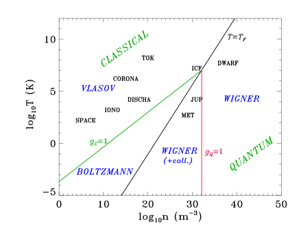
Figure 1: Plasma diagram in the $\log T-\log n$ plane. IONO: ionospheric plasma; SPACE: interstellar space; CORONA: solar corona; DISCHA: typical electric discharge; TOK: tokamak experiment (magnetic confinement fusion); ICF: inertial confinement fusion; MET: metals and metal clusters; JUP: Jupiter’s core; DWARF: white dwarf star.

The $\log T-\log n$ plane is divided into four regions, two of which are classical (above the $T=T_{F}$ line) and two quantum. Each quantum/classical region is then divided in two collisional/collisionless subregions, identified by the kinetic equations that are relevant to each regime. As we shall see in the forthcoming sections, the Vlasov and Wigner equations are the appropriate models respectively for collisionless classical and collisionless quantum plasmas. ‘Boltzmann’ is used as a generic term for collisional kinetic equations in the classical regime. Collisional effects in the quantum regime are much harder to deal with, and no uncontroversial kinetic model exists in that regime, which is identified by ‘Wigner (+ coll.)’ on the figure.

We point out that all previous considerations have implicitly assumed thermal equilibrium. Out-of-equilibrium regimes should be treated much more carefully and the above results may not be entirely correct. For example, if an electron beam is injected into a plasma, the beam velocity will have to be taken into account when determining the de Broglie wavelength, which will therefore be smaller. For this reason, systems that are far from equilibrium can sometimes be treated with a semiclassical model, even though the corresponding equilibrium may still be fully quantum (see Sec. 4.4).

Several points corresponding to natural and laboratory plasmas have also been plotted in Fig. 1. We note that space and magnetic fusion plasmas fall in the classical collisionless region, whereas inertial confinement fusion plasmas may display quantum and/or strong coupling effects. Extremely dense astrophysical objects such as white dwarf stars are definitely quantum and collisionless, even though they are as hot as fusion or solar plasmas.

3 Electrons in metals and metallic nanostructures: Pauli blocking

The typical quantum coupling parameter for ordinary metals is larger than unity, so that, in principle, electron-electron collisions are as important as collective effects. If that were really the case, one should abandon collisionless models altogether and resort to the full $N$-body problem. This is hardly a feasible task. Fortunately, however, the effect known as Pauli blocking reduces the collision rate quite dramatically in most cases of interest. This occurs when the electron distribution is close to the Fermi-Dirac equilibrium at relatively low temperatures. The fundamental point is that, when all lower levels are occupied, the exclusion principle forbids a vast number of transitions that would otherwise be possible [14]. In particular, at strictly zero temperature, all electrons have energies below $E_{F}$, and no transition is possible, simply because there are no available states for the electrons to occupy. At moderate temperatures, only electrons within a shell of thickness $k_{B}T$ about the Fermi surface (i.e. the region where $E=E_{F}$) can undergo collisions (this shell is delimited by the two vertical lines in Fig. 2). For such electrons, the e-e collision rate (inverse of the lifetime $\tau_{ee}$) is proportional to $k_{B}T/\hbar$ (this is a form of the uncertainty principle, energy $\times$ time = const.). The average collision rate is obtained by multiplying the previous expression by the fraction of electrons present in the shell of thickness $T$ about the Fermi surface, which is $\sim T/T_{F}$. One obtains

$$\nu_{ee}\sim~{}\frac{k_{B}T^{2}}{\hbar~{}T_{F}}~{}.$$ (3.1)

In normalized units, this expression reads as

$$\frac{\nu_{ee}}{\omega_{p}}=\frac{E_{F}}{\hbar\omega_{p}}~{}\left(\frac{T}{T_{F}}\right)^{2}=\frac{1}{g_{Q}^{1/2}}~{}\left(\frac{T}{T_{F}}\right)^{2}$$ (3.2)

Thus, $\nu_{ee}<\omega_{p}$ in the region where $T<T_{F}$ and $g_{Q}>1$, which is the relevant one for metallic electrons (Fig. 1). Restoring dimensional units, we find that, at room temperature, $\tau_{ee}\simeq 10^{-10}~{}{\rm s}$, which is much larger than the typical collisionless time scale $\tau_{p}=2\pi\omega_{p}^{-1}\simeq 10^{-15}~{}{\rm s}=1~{}{\rm fs}$. In addition, the typical time scale for electron-lattice collisions $\tau_{ei}\simeq 10^{-14}~{}{\rm s}=10~{}{\rm fs}$ is also larger than $\tau_{p}$. Therefore, it appears that a collisionless regime is indeed relevant on a time scale of the order of the femtosecond.

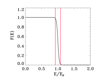
Figure 2: Fermi-Dirac energy distribution for a case with $T/T_{F}=0.1$. The vertical lines define a shell of thickness $k_{B}T$ around the Fermi surface.

A word of caution is in order, however, not to overestimate the effect of Pauli blocking. The above considerations are valid at thermodynamic equilibrium, whereas many more transitions are allowed for out-of-equilibrium electrons. Therefore, for strongly excited systems where many nonequilibrium electrons are present, the collision frequency may be larger than the simple estimate given in (3.2).

Some typical parameters for metallic electrons (gold) at room temperature are summarized in Table 1. We note that $\tau_{p}$, the typical collisionless time scale, is of the order of the femtosecond. With the recent development of ultrafast laser sources with femtosecond period, it is therefore possible to probe the mean-field properties of metallic nanostructures. For example, the electron dynamics in thin gold films excited with femtosecond lasers was studied experimentally in several works [2, 3]. We also point out that $\lambda_{F}$, the typical collisionless length scale, is of the order of the Ångstrom, which is comparable to the typical atomic size.

Table 1: Typical parameters for electrons in gold at room temperature

$n$	$5.9\times 10^{28}~{}{\rm m}^{-3}$
$T$	$300$ K
$\omega_{p}$	$1.37\times 10^{16}~{}{\rm s^{-1}}$
$\tau_{p}$	$0.46~{}{\rm fs}$
$\tau_{ie}$	$30~{}{\rm fs}$
$T_{F}$	$6.4\times 10^{4}~{}{\rm K}$
$E_{F}$	$5.53~{}{\rm eV}$
$v_{F}$	$1.4\times 10^{6}~{}{\rm ms^{-1}}$
$\lambda_{F}$	$1\times 10^{-10}~{}{\rm m}$
$g_{Q}$	12.7
$r_{s}/a_{0}$	3

4 Models

The most fundamental model for the quantum $N$-body problem is the Schrödin- ger equation for the $N$-particle wave function $\psi(x_{1},x_{2},\dots,x_{N},t)$. Obviously, this is an unrealistic task, both for analytical calculations and numerical simulations. A drastic, but useful and to some extent plausible, simplification can be achieved by neglecting two-body (and higher order) correlations. This amounts to assume that the $N$-body wave function can be factored into the product of $N$ one-body functions:

$$\psi(x_{1},x_{2},\dots,x_{N},t)=\psi_{1}(x_{1},t)~{}\psi_{2}(x_{2},t)\dots\psi_{N}(x_{N},t).$$ (4.1)

For fermions, a weak form of the exclusion principle is satisfied if none of the wave functions on the right-hand side of (4.1) are identical .

The assumption of weak correlation between the particles is satisfied, as we have seen, when the quantum coupling parameter $g_{Q}$ is small. The set of $N$ one-body wave functions is known as a quantum mixture (or quantum mixed state) and is usually represented by a density matrix

$$\rho(x,y,t)=\sum_{\alpha=1}^{N}p_{\alpha}\psi_{\alpha}(x,t)~{}\psi_{\alpha}^{\displaystyle*}(y,t),$$ (4.2)

where, for clarity, we have assumed the same normalization $\int\vline\psi_{\alpha}\vline^{2}dx=1$ for all wave functions and then introduced the occupation probabilities $p_{\alpha}$.

Both the Wigner and Hartree models described below are completely equivalent to models based on the density matrix formalism (Von Neumann equation).

4.1 Wigner-Poisson

The Wigner representation [16] is a useful tool to express quantum mechanics in a phase space formalism (for reviews see [17, 18, 19]). As detailed above, a generic quantum mixed state can be described by $N$ single-particle wave functions $\psi_{\alpha}(x,t)$ each characterized by a probability $p_{\alpha}$ satisfying $\sum_{\alpha=1}^{N}p_{\alpha}=1$. The Wigner function is a function of the phase space variables $(x,v)$ and time, which, in terms of the single-particle wave functions, reads as

$$f(x,v,t)=\sum_{\alpha=1}^{N}\frac{m}{2\pi\hbar}~{}p_{\alpha}\int_{-\infty}^{+\infty}\psi_{\alpha}^{\displaystyle*}\left(x+\frac{\lambda}{2},t\right)\psi_{\alpha}\left(x-\frac{\lambda}{2},t\right)e^{imv\lambda/\hbar}~{}d\lambda$$ (4.3)

(we restrict our discussion to one-dimensional cases, but all results can easily be generalized to three dimensions). It must be stressed that the Wigner function, although it possesses many useful properties, is not a true probability density, as it can take negative values. However, it can be used to compute averages just like in classical statistical mechanics. For example, the expectation value of a generic quantity $A(x,v)$ is defined as:

$$\langle A\rangle=\frac{\int\int f(x,v)A(x,v)dxdv}{\int\int f(x,v)dxdv},$$ (4.4)

and yields the correct quantum-mechanical value . In addition, the Wigner function reproduces the correct quantum-mechanical marginal distributions, such as the spatial density:

$$n(x,t)=\int_{-\infty}^{+\infty}f(x,v,t)~{}dv=\sum_{\alpha=1}^{N}p_{\alpha}\mid\psi_{\alpha}\mid^{2}.$$ (4.5)

We also point out that, of course, not all functions of the phase space variables are genuine Wigner functions, as they cannot necessarily be written in the form (4.3). In general, although it is trivial to find the Wigner function given the $N$ wave functions that define the quantum mixture, the inverse operation is not generally feasible. Indeed, there are no simple rules to establish whether a given function of $x$ and $v$ is a genuine Wigner function. For a more detailed discussion on this issue, and some practical recipes to construct genuine Wigner functions, see [20].

The Wigner function obeys the following evolution equation:

$$\frac{\partial{f}}{\partial{t}}+v\frac{\partial{f}}{\partial{x}}~{}+$$

$$\frac{em}{2i\pi\hbar^{2}}\int\int{d\lambda}~{}{dv^{\prime}}e^{im(v-v^{\prime})\lambda/\hbar}\left[\phi\left(x+\frac{\lambda}{2}\right)-\phi\left(x-\frac{\lambda}{2}\right)\right]f(x,v^{\prime},t)=0~{},$$ (4.6)

where $\phi(x,t)$ is the self-consistent electrostatic potential. Developing the integral term in (4.6) up to order $O(\hbar^{2})$ we obtain

$$\frac{\partial{f}}{\partial{t}}+v\frac{\partial{f}}{\partial{x}}-\frac{e}{m}\frac{\partial\phi}{\partial{x}}\frac{\partial{f}}{\partial{v}}=\frac{e\hbar^{2}}{24m^{3}}\frac{\partial^{3}\phi}{\partial{x^{3}}}\frac{\partial^{3}{f}}{\partial{v^{3}}}+O(\hbar^{4})$$ (4.7)

The Vlasov equation is thus recovered in the formal semiclassical limit $\hbar\to 0$. We stress, however, that rigorous asymptotic results are much harder to obtain and generally involve weak convergence.

The Wigner equation must be coupled to the Poisson’s equation for the electric potential

$$\frac{\partial^{2}\phi}{\partial x^{2}}=\frac{e}{\varepsilon_{0}}\left(\int fdv-n_{0}\right)~{},$$ (4.8)

where we have assumed that the ions form a motionless neutralizing background with uniform density $n_{0}$ (this is known as the ‘jellium’ model in solid state physics).

The resulting Wigner-Poisson (WP) system has been extensively used in the study of quantum transport [6, 7, 21]. Exact analytical results can be obtained by linearizing (4.6) and (4.8) around a spatially homogeneous equilibrium given by $f_{0}(v)$. By expressing the fluctuating quantities as a sum of plane waves $\exp(ikx-i\omega t)$ with frequency $\omega$ and wave number $k$, the dispersion relation can be written in the form $\varepsilon(k,\omega)=0$, where the dielectric constant $\varepsilon$ reads, for the WP system,

$$\varepsilon_{\rm WP}(\omega,k)=1+\frac{m\omega_{p}^{2}}{n_{0}k}\int\frac{f_{0}(v+\hbar k/2m)-f_{0}(v-\hbar k/2m)}{\hbar k(\omega-kv)}~{}dv~{}.$$ (4.9)

With an appropriate change of integration variable, (4.9) can be written as

$$\varepsilon_{\rm WP}(\omega,k)=1-\frac{\omega_{p}^{2}}{n_{0}}\int\frac{f_{0}(v)}{(\omega-kv)^{2}-\hbar^{2}k^{4}/4m^{2}}~{}dv~{}.$$ (4.10)

From (4.9), one can recover the Vlasov-Poisson (VP) dispersion relation by taking the semiclassical limit $\hbar\to 0$

$$\varepsilon_{\rm VP}(\omega,k)=1+\frac{\omega_{p}^{2}}{n_{0}k}\int\frac{\partial f_{0}/\partial v}{\omega-kv}~{}dv~{}.$$ (4.11)

The integration in (4.9) and (4.11) should be performed along the Landau contour in the complex (Re$~{}v$, Im$~{}v$) plane, so that the singularity at $v=\omega/k$ is always left above the contour [12]. This prescription allows one to obtain the correct imaginary part of $\varepsilon(k,\omega)$, which is at the basis of the phenomenon of Landau damping.

Just like in the classical case (Vlasov-Poisson), the dispersion relation (4.9) can also support unstable solutions, i.e. solutions with a positive imaginary part of the frequency. These solutions grow exponentially until some nonlinear effect kicks in and leads to saturation of the instability. The stability property of the dispersion relation of the Wigner-Poisson system have been extensively studied in [22, 23].

4.2 Hartree

A completely equivalent approach to the WP system is obtained by making direct use of the $N$ wave functions $\psi_{\alpha}(x,t)$. These obey $N$ independent Schrödinger equations, coupled through Poisson’s equation

$$i\hbar\frac{\partial\psi_{\alpha}}{\partial\,t} = -\frac{\hbar^{2}}{2m}\frac{\partial^{2}\psi_{\alpha}}{\partial x^{2}}-e\phi\psi_{\alpha}~{},~{}~{}~{}~{}~{}\alpha=1\dots N$$ (4.12)

$$\frac{\partial^{2}\phi}{\partial x^{2}} = \frac{e}{\varepsilon_{0}}\left(\sum_{\alpha=1}^{N}p_{\alpha}|\psi_{\alpha}|^{2}-n_{0}\right)~{}.$$ (4.13)

This type of model was originally derived by Hartree in the context of atomic physics, with the aim of studying the self-consistent effect of atomic electrons on the Coulomb potential of the nucleus. Subsequently, Fock introduced a correction that accounts for the parity of the $N$-particle wave function for an ensemble of fermions (Hartree-Fock model), but this development will not be considered in this paper .

Instead, it is useful to think of the above Schrödinger-Poisson equations (4.12)–(4.13) as the quantum-mechanical analog of Dawson’s multistream model [26]. Dawson supposed that the classical distribution function can be represented as a sum of $N$ ‘streams’, each characterized by a probability $p_{\alpha}$, a density $n_{\alpha}$, and a velocity $u_{\alpha}$:

$$f(x,v,t)=\sum_{\alpha=1}^{N}p_{\alpha}~{}n_{\alpha}(x,t)~{}\delta(v-u_{\alpha}(x,t))~{},$$ (4.14)

where $\delta$ stands for the Dirac delta. The streams represent infinitely thin filaments in phase space. If $f$ obeys the Vlasov equation, then the functions $n_{\alpha}$ and $u_{\alpha}$ each satisfy the following continuity and momentum conservation equations:

$$\frac{\partial\,n_{\alpha}}{\partial\,t}+\frac{\partial}{\partial\,x}(n_{\alpha}u_{\alpha}) = 0\,,$$ (4.15)

$$\frac{\partial\,u_{\alpha}}{\partial\,t}+u_{\alpha}\frac{\partial\,u_{\alpha}}{\partial x} = \frac{e}{m}\frac{\partial\phi}{\partial\,x}~{},$$ (4.16)

coupled of course to Poisson’s equation with the electron density given by $n(x,t)=\sum_{\alpha}p_{\alpha}n_{\alpha}(x,t)$. Note that the representation (4.14) presents some drawbacks, as the functions $u_{\alpha}(x,t)$ can become multivalued during the time evolution. This means that the system (4.15)–(4.16) will develop singularities, such as an infinite density at certain positions. When this happens, the fluid description (4.15)–(4.16) ceases to be valid, although the phase space picture of the streams is still correct.

This line of reasoning can be extended to the quantum case [27, 28] by applying the Madelung representation of the wave function to the system (4.12)–(4.13). Let us introduce the real amplitude $A_{\alpha}(x,t)$ and the real phase $S_{\alpha}(x,t)$ associated to the pure state $\psi_{\alpha}$ according to

$$\psi_{\alpha}=A_{\alpha}\exp({i\,S_{\alpha}/\hbar})\,.$$ (4.17)

The density $n_{\alpha}$ and the velocity $u_{\alpha}$ of each stream are given by

$$n_{\alpha}=|\psi_{\alpha}|^{2}=A_{\alpha}^{2}\,,\qquad u_{\alpha}=\frac{1}{m}\frac{\partial\,S_{\alpha}}{\partial\,x}\,.$$ (4.18)

Introducing Eqs. (4.17)–(4.18) into Eqs. (4.12)–(4.13) and separating the real and imaginary parts of the equations, we find

$$\frac{\partial\,n_{\alpha}}{\partial\,t}+\frac{\partial}{\partial\,x}(n_{\alpha}u_{\alpha}) = 0\,,$$ (4.19)

$$\frac{\partial\,u_{\alpha}}{\partial\,t}+u_{\alpha}\frac{\partial\,u_{\alpha}}{\partial x} = \frac{e}{m}\frac{\partial\phi}{\partial\,x}+\frac{\hbar^{2}}{2m^{2}}\frac{\partial}{\partial\,x}\left(\frac{\partial^{2}(\sqrt{n_{\alpha}})/\partial\,x^{2}}{\sqrt{n_{\alpha}}}\right)\,.$$ (4.20)

Quantum effects are contained in the $\hbar$-dependent term in (4.20) (sometimes called the Bohm potential). If we set $\hbar=0$, we obviously obtain the classical multistream model (4.15)–(4.16). An attractive feature of the quantum multistream model is that, contrarily to its classical counterpart, it does not generally develop singularities. This is thanks to the Bohm potential, which, by introducing a certain amount of wave dispersion, prevents the density to build up indefinitely.

Linearizing equations (4.19)–(4.20) (supplemented by Poisson’s equation) around the spatially homogeneous equilibrium: $n_{\alpha}=n_{0}$, $u_{\alpha}=u_{0\alpha}$ and $\phi=0$, one obtains the following dielectric constant

$$\varepsilon_{\rm H}(\omega,k)=1-\sum_{\alpha=1}^{N}p_{\alpha}~{}\frac{\omega_{p}^{2}}{(\omega-ku_{0\alpha})^{2}-\hbar^{2}k^{4}/4m^{2}}.$$ (4.21)

The classical multistream relation is obtained simply by setting $\hbar=0$ in (4.21).

The equivalence of the Wigner-Poisson and Hartree models can be readily proven on the linear dispersion relation. The homogeneous equilibrium described above corresponds to wave functions

$$\psi_{\alpha}=\sqrt{n_{0}}~{}\exp\left(i\frac{mu_{0\alpha}}{\hbar}~{}x\right).$$ (4.22)

The Wigner transform (4.3) of the above wave functions (4.22) is given by the following expression

$$f_{0}(v)=\sum_{\alpha=1}^{N}p_{\alpha}n_{0}\delta(v-u_{0\alpha}),$$ (4.23)

where $\delta$ stands for the Dirac delta. By inserting (4.23) into the WP dispersion relation (4.9), one recovers precisely the multistream dispersion relation (4.21).

4.3 Fluid model

In classical plasma physics, fluid (or hydrodynamic) models are often derived by taking moments of the appropriate kinetic equation (e.g. Vlasov’s equation) in velocity space. The moment of order $s$ is defined as:

$$M_{s}(x,t)=\int_{-\infty}^{+\infty}f(x,v,t)v^{s}dv.$$ (4.24)

Then, the zeroth order moment is the spatial density and obeys the continuity equation; the first order moment is the average velocity and obeys a momentum conservation equation; the second order moment is related to the pressure, and so on. This procedure generates an infinite number of fluid equations, which is usually truncated at a relatively low order by assuming an appropriate closure equation. The closure often takes the form of a thermodynamic equation of state, relating the pressure to the density, e.g. the polytropic relation $P\propto n^{\gamma}$. The same procedure can be applied to the Wigner equation, although some steps in the derivation are somewhat subtler than in the classical case. With this technique, quantum fluid equations were derived in [29]. Here, we shall present a succinct derivation of the same fluid model using a different approach based on the Hartree equations [30, 31].

The starting point is the system of $2N$ equations (4.19)–(4.20), which is completely equivalent to Hartree’s model (4.12)–(4.13). Let us define the global density $n(x,t)$

$$n(x,t)=\sum_{\alpha=1}^{N}p_{\alpha}n_{\alpha}$$ (4.25)

and the global average velocity $u(x,t)$

$$u(x,t)\equiv\langle u_{\alpha}\rangle=\sum_{\alpha=1}^{N}p_{\alpha}\frac{n_{\alpha}}{n}~{}u_{\alpha}$$ (4.26)

By multiplying the continuity equation (4.19) by $p_{\alpha}$ and summing over $\alpha=1\dots N$, we obtain

$$\frac{\partial\,n}{\partial\,t}+\frac{\partial(nu)}{\partial x}=0$$ (4.27)

Similarly, for the equation of momentum conservation (4.20), one obtains

$$\frac{\partial\,u}{\partial\,t}+u\frac{\partial u}{\partial x}=\frac{e}{m}\frac{\partial\phi}{\partial x}+\frac{\hbar^{2}}{2m^{2}}~{}\frac{\partial}{\partial x}\sum_{\alpha=1}^{N}p_{\alpha}\left(\frac{\partial_{x}^{2}\sqrt{n_{\alpha}}}{\sqrt{n_{\alpha}}}\right)-\frac{1}{mn}\frac{\partial P}{\partial x}$$ (4.28)

where the pressure $P(x,t)$ is defined as

$$P=mn\left[\frac{\sum_{\alpha}p_{\alpha}n_{\alpha}u^{2}_{\alpha}}{n}-\left(\frac{\sum_{\alpha}p_{\alpha}n_{\alpha}u_{\alpha}}{n}\right)^{2}\right]\equiv mn(\langle u_{\alpha}^{2}\rangle-\langle u_{\alpha}\rangle^{2})$$ (4.29)

So far the derivation is exact, but (4.28) still involves a sum over the $N$ states, so no simplification was achieved. Our purpose is to obtain a closed system of two equations for the global averaged quantities $n$ and $u$. In order to close the system, two approximations are needed:

1. We postulate a classical equation of state, relating the pressure to the density: $P=P(n)$.

2. We assume that the following substitution is allowed:

   $$\sum_{\alpha=1}^{N}p_{\alpha}\left(\frac{\partial_{x}^{2}\sqrt{n_{\alpha}}}{\sqrt{n_{\alpha}}}\right)~{}\Longrightarrow~{}\frac{\partial_{x}^{2}\sqrt{n}}{\sqrt{n}}$$ (4.30)

It can be shown that the second hypothesis is satisfied for length scales larger than $\lambda_{F}$. This will be apparent from the linear theory detailed in Sec. 5.

With these assumptions, we obtain the following reduced system of fluid equations for the global quantities $n$ and $u$

$$\frac{\partial\,n}{\partial\,t}+\frac{\partial(nu)}{\partial x}=0$$ (4.31)

$$\frac{\partial\,u}{\partial\,t}+u\frac{\partial u}{\partial x}=\frac{e}{m}\frac{\partial\phi}{\partial x}+\frac{\hbar^{2}}{2m^{2}}~{}\frac{\partial}{\partial x}\left(\frac{\partial_{x}^{2}\sqrt{n}}{\sqrt{n}}\right)-\frac{1}{mn}\frac{\partial P}{\partial x}$$ (4.32)

where $\phi$ is given by Poisson’s equation. We stress that we have transformed a system of $2N$ equations (4.19)–(4.20) into a system of just two equations.

An interesting form of the system (4.31)–(4.32) can be obtained by introducing the following ‘effective’ wave function

$$\Psi(x,t)=\sqrt{n(x,t)}\exp{(iS(x,t)/\hbar)},$$ (4.33)

where $S(x,t)$ is defined according to the relation $mu=\partial_{x}S$, and $n=|\Psi|^{2}$. It is easy to show that (4.31)–(4.32) is equivalent to the following nonlinear Schrödinger equation

$$i\hbar\frac{\partial\Psi}{\partial\,t}=-\,\frac{\hbar^{2}}{2m}~{}\frac{\partial^{2}\Psi}{\partial x^{2}}-e\phi\Psi+W_{{\rm eff}}(|\Psi|^{2})~{}\Psi.$$ (4.34)

$W_{{\rm eff}}(n)$ is an effective potential related to the pressure $P(n)$

$$W_{\rm eff}(n)=\int^{n}\frac{dn^{\prime}}{n^{\prime}}\frac{dP(n^{\prime})}{dn^{\prime}}.$$ (4.35)

As an example, let us consider a one-dimensional (1D) zero-temperature fermion gas, whose equation of state is a polytropic with exponent $\gamma=3$

$$P=\frac{mv_{F}^{2}}{3n_{0}^{2}}n^{3},$$ (4.36)

where $v_{F}$ is the Fermi velocity computed with the equilibrium density $n_{0}$. Using (4.36), the effective potential becomes

$$W_{\rm eff}=\frac{mv_{F}^{2}}{2n_{0}^{2}}|\Psi|^{4}\,.$$ (4.37)

This fluid model is a useful approximation, as it reduces dramatically the complexity of the Hartree system ($2N$ equations) or the Wigner equation (phase space dynamics). Its validity is limited to systems that are large compared to $\lambda_{F}$. Like all fluid approximations, it neglects typical kinetic phenomena originating from the details of the phase space distribution function. In particular, it cannot reproduce Landau’s collisionless damping.

4.4 Vlasov-Poisson

The Wigner and Hartree approaches are both kinetic and quantum. The above fluid model was derived by dropping kinetic effects, while preserving quantum effects through the Bohm potential. Another possible approximation could consist in neglecting quantum effects while keeping kinetic ones. The resulting semiclassical limit is, of course, given by the Vlasov equation

$$\frac{\partial{f}}{\partial{t}}+v\frac{\partial{f}}{\partial{x}}-\frac{e}{m}\frac{\partial\phi}{\partial{x}}\frac{\partial{f}}{\partial{v}}=0,$$ (4.38)

coupled, as usual, to Poisson’s equation.

The Vlasov-Poisson (VP) system has been used to study the dynamics of electrons in metal clusters and thin metal films [1, 32]. It is appropriate for large excitation energies, for which the electrons’ de Broglie wavelength is relatively small, thus reducing the importance of quantum effects in the electron dynamics. However, as we have seen in Sec. 2.2, the equilibrium distribution for electrons in metals lies deeply in the quantum region ($g_{Q}\gtrsim 1$), so that the initial condition must be given by a quantum Fermi-Dirac distribution. In this sense, the VP system is semiclassical.

4.5 Initial and boundary conditions

In order to perform numerical simulations, boundary and initial conditions must be specified. Physically, the initial condition should represent a situation of thermodynamics equilibrium (ground state). For electrons in metals, most analytical results are obtained in the case of an infinite system (often referred to as the ‘bulk’ in solid state physics), which can be realized in practice by taking periodic boundary conditions with spatial period $L$ (this, of course, introduces a lower bound for the wave numbers, namely $k_{0}=2\pi/L$). For such an infinite system, the ground state can be easily specified. For the WP and VP models, any function of the velocity only $f_{0}(v)$ constitutes a stationary state. In particular, for fermions we take the Fermi-Dirac distribution (see, however, Sec. 5.2 for a discussion on the appropriate Fermi-Dirac distribution for 1D problems):

$$f_{0}(v)={\rm const.}\times\frac{1}{1+e^{\beta_{e}(\epsilon-\mu)}},$$ (4.39)

where $\beta_{e}=1/k_{B}T_{e}$ and $\epsilon=mv^{2}/2$ is the single-particle energy (here, $v$ is the modulus of the 3D velocity vector). The chemical potential $\mu(T)$ is determined so that $\int f_{0}dv=n_{0}$, where $n_{0}$ is the equilibrium density; $\mu$ becomes equal to the Fermi energy $E_{F}$ in the limit $T\to 0$. The same ground state can be defined for the Hartree model by choosing the initial wave functions in the form (4.22). The Fermi-Dirac distribution is then specified by the probabilities $p_{\alpha}=[1+e^{\beta_{e}(\epsilon_{\alpha}-\mu)}]^{-1}$, with $\epsilon_{\alpha}=mu_{0\alpha}^{2}/2$.

The bulk approximation is not relevant for metal clusters and other metallic nanostructures, which are small isolated objects that exist either in vacuum or embedded in a background non-metallic matrix. For open quantum systems (Wigner or Hartree), the choice of appropriate boundary conditions is a subtle issue, which will not be addressed here [33]. For the semiclassical VP system, one can, for instance, use open boundaries for the Vlasov equation (zero incoming flux) and Dirichlet conditions for the Poisson equation.

As to the initial condition, the ground state is easily determined for the VP system with open boundaries. The main difference from the bulk equilibrium is that, for an open system, the electrostatic energy does not vanish and the equilibrium density $n_{0}(x)$ is position dependent. As any function of the total energy is a stationary solution of the Vlasov equation, we define the initial state as a Fermi-Dirac distribution (4.39) with $\epsilon(x,v)=mv^{2}/2-e\phi(x)$, where the potential $\phi$ is not yet known. By plugging this Fermi-Dirac distribution into Poisson’s equation, one obtains a nonlinear equation that can be solved iteratively to obtain $\phi$, which in turns yields the ground state distribution.

In contrast, stationary solutions of the Wigner equations are not simply given by functions of the energy, so that the above procedure cannot be applied. It is easier to compute the ground state in terms of the Hartree wave functions $\psi_{\alpha}$, and then compute the corresponding Winger function with (4.3). Several methods to compute the ground state wave functions in the Hartree formalism are available in the literature [34, 35, 36] and will not be discussed here.

5 Linear theory

In order to compare the various models described in Sec. 4, we shall go into some details of the linear theory for a zero-temperature homogeneous equilibrium with periodic boundaries, both in 1D and in 3D. More detailed calculations on the linear theory of quantum plasmas can be found in [25, 37, 38].

5.1 Zero-temperature 1D Fermi-Dirac equilibrium

In one spatial dimension, the Fermi-Dirac distribution at $T=0$ is given by $f_{0}(v)=n_{0}/2v_{F}$ if $|v|\leq v_{F}$ and $f_{0}(v)=0$ if $|v|>v_{F}$. The Fermi velocity in 1D is

$$v_{F}=\frac{\pi}{2}\frac{\hbar n_{0}}{m}.$$ (5.1)

This distribution is identical to the so-called ‘water-bag’ distribution, which has been extensively used in classical plasma physics [39]. Using the Wigner linear dielectric constant (4.10) and developing the results in powers of $k$ and $\hbar$, one obtains the following dispersion relation (details are given in [29])

$$\omega^{2}=\omega_{p}^{2}+k^{2}v_{F}^{2}+\frac{\hbar^{2}k^{4}}{4m^{2}}+\frac{\hbar^{2}k^{6}\lambda_{F}^{2}}{3m^{2}}+O(\hbar^{4},k^{12})\,.$$ (5.2)

With the Vlasov dielectric constant, the dispersion relation for the same equilibrium reads as

$$\omega^{2}=\omega_{p}^{2}+k^{2}v_{F}^{2}\,.$$ (5.3)

Note that the above Vlasov dispersion relation is exact: no terms of order $k^{4}$ or higher exist. We also point out that, for this 1D equilibrium, the imaginary part of the dielectric constant vanishes identically and therefore there is no Landau damping.

We now want to compare the above result (5.2), obtained with the ‘exact’ Wigner-Poisson model, with the equivalent result obtained with the fluid model developed in Sec. 4.3. Let us consider the fluid equations (4.31)-(4.32) in the case of a zero-temperature 1D fermion gas, for which the pressure is given by (4.36). Linearizing around the homogeneous equilibrium $n=n_{0}$, $u=\phi=0$, one obtains the following dispersion relation (no further approximation has been used)

$$\omega^{2}=\omega_{p}^{2}+k^{2}v_{F}^{2}+\frac{\hbar^{2}k^{4}}{4m^{2}}\,.$$ (5.4)

We see that the fluid (5.4) and the Wigner (5.2) dispersion relations coincide up to terms of order $k^{4}$. This confirms our conjecture that the fluid model is a good approximation of the WP (or Hartree) model in the limit of long wavelengths.

5.2 Zero-temperature 3D Fermi-Dirac equilibrium

From a physical point of view, it is possible to imagine a real physical system that displays 1D behavior. This can be realized, for instance, in a thin metal film where the dimensions parallel to the surfaces are much larger than the thickness of the film. The electron dynamics can then be described by a 1D infinite slab model depending only on the co-ordinate $x$ normal to the film surfaces. Even in such a situation, however, the 1D Fermi-Dirac distribution discussed in Sec. 5.1 is not realistic. Indeed, in the ground state at zero temperature, the electrons occupy all the available quantum states up to the Fermi surface, defined by $\vline~{}v~{}\vline\leq v_{F}$. There is no reason why states with $v_{y}\neq 0$ and $v_{z}\neq 0$ should not be available, and indeed they are occupied. Therefore, the equilibrium distribution is always three-dimensional, even in a 1D infinite slab geometry:

$$f_{0}^{\rm 3D}(v)=\frac{n_{0}}{\frac{4}{3}\pi v_{F}^{3}}~{}{\rm for}~{}|v|\leq v_{F},~{}~{}~{}~{}{\rm and}~{}~{}~{}~{}f_{0}^{\rm 3D}(v)=0~{}{\rm for}~{}|v|>v_{F}.$$ (5.5)

However, it is still possible to keep the 1D geometry for the Vlasov and Poisson’s equations, provided that one uses, as initial condition, the 3D Fermi-Dirac distribution (5.5) projected on the $v_{x}$ axis: $f_{0}^{\rm 1D}(v_{x})=\int\int f_{0}^{\rm 3D}dv_{y}dv_{z}$. This yields (we now write $v$ for $v_{x}$)

$$f_{0}^{\rm 1D}(v)=\frac{3}{4}\frac{n_{0}}{v_{F}}\left(1-\frac{v^{2}}{v_{F}^{2}}\right)~{}{\rm for}~{}|v|\leq v_{F},~{}~{}~{}~{}{\rm and}~{}~{}~{}~{}f_{0}^{\rm 1D}(v)=0~{}{\rm for}~{}|v|>v_{F}.$$ (5.6)

This approach is not as contrived as it might appear at first sight. Indeed, linear wave propagation in a collisionless plasma is intrinsically a 1D phenomenon, which involves plane waves traveling in a well-defined direction. In computing the dispersion relation from the 3D equivalent of (4.10) or (4.11), we would first integrate over the two velocity dimensions normal to the direction of wave propagation (which can, arbitrarily and without loss of generality, be chosen to be the $v_{x}$ direction). Therefore, we would be left with a reduced distribution such as (5.6) that intervenes in a 1D dispersion relation such as (4.10) or (4.11). This line of reasoning is no more valid when nonlinear effects become important, as these may trigger truly 3D phenomena. Collisions also constitute an intrinsically 3D effect.

We now insert (5.6) into (4.10) or (4.11) and compute the dispersion relations for the WP and VP systems, developed in powers of $k$. For the equilibrium (5.6), the dielectric constant does display an imaginary part, and therefore there is, in principle, some collisionless damping associated with this equilibrium; however, we shall neglect it for the moment and concentrate on the real part of $\varepsilon(k,\omega)$. We also assume the following ordering

$$\frac{\hbar k}{m}\ll v_{F}\ll\frac{\omega}{k},$$ (5.7)

which is valid for long wavelengths. Note that the second inequality in (5.7) means that the phase velocity of the wave must be greater than the Fermi velocity. With this assumption, the dispersion relation up to fourth order in $k$ reads as

$$\omega^{2}=\omega_{p}^{2}+\frac{3}{5}~{}k^{2}v_{F}^{2}+\frac{\hbar^{2}k^{4}}{4m^{2}}+\dots\,.$$ (5.8)

Let us now derive the dispersion relation for the quantum fluid model (4.31)-(4.32), by assuming an equation of state of the form:

$$\frac{P}{P_{0}}=\left(\frac{n}{n_{0}}\right)^{\gamma},$$ (5.9)

where $P_{0}$ and $n_{0}$ are the equilibrium pressure and density, respectively. We obtain:

$$\omega^{2}=\omega_{p}^{2}+\gamma k^{2}v_{0}^{2}+\frac{\hbar^{2}k^{4}}{4m^{2}}~{},$$ (5.10)

where $v_{0}^{2}=P_{0}/(mn_{0})$. We note that the 1D fluid dispersion relation (5.4) is recovered correctly when $\gamma=3$ and $P_{0}=n_{0}~{}mv_{F}^{2}/3$ as can be deduced from (4.36). Now, in 3D, the pressure of a quantum electron gas at thermal equilibrium and zero temperature can be written as [13]

$$P_{0}=\frac{2}{5}n_{0}E_{F}$$ (5.11)

(where $E_{F}$ is computed at equilibrium), so that $v_{0}^{2}=v_{F}^{2}/5$ and (5.10) becomes

$$\omega^{2}=\omega_{p}^{2}+\frac{\gamma}{5}k^{2}v_{0}^{2}+\frac{\hbar^{2}k^{4}}{4m^{2}}~{}.$$ (5.12)

One may think that the correct exponent to use in the equation of state (5.9) is $\gamma=(D+2)/D$, yielding 5/3 in three dimensions. However, with this choice, the fluid dispersion relation (5.12) would differ from the WP result (5.8). The correct result is obtained by taking $\gamma=3$, just like in the 1D case. Why is it so? The reason, as was already mentioned earlier, is that linear wave propagation is essentially a 1D phenomenon, because it involves propagation along a single direction, without any energy exchanges in the other two directions. The details of the linear dynamics are essentially determined by the equation of state, which must therefore feature the 1D exponent. In contrast, the equilibrium is truly 3D (because we have projected the 3D Fermi-Dirac distribution over the $x$ direction): therefore, the equilibrium pressure must indeed be given by its 3D expression (5.11).

5.3 Finite temperature solutions: Landau damping

So far, we have completely neglected the fact, discovered by Landau in 1940 [40], that electrostatic waves can be exponentially damped even in the absence of any collisions. The rigorous theory of Landau damping can be found in most plasma physics textbooks. Here, we shall only remind the reader that the damping originates from the singularity appearing in the dispersion relations (4.9) and (4.11) at the point $v=\omega/k$ in velocity space. This corresponds to particles whose velocity is equal to the phase velocity of the wave $\omega/k$ (resonant particles). Landau showed that the correct way to perform the integral in the dispersion relation is not simply to take the principal value (which only yields the real part of the frequency), but to integrate in the complex $v$ plane, following a contour that leaves the singularity always on the same side. With this prescription, the dielectric function is found to possess an imaginary part, which in turn gives rise to a damping rate $\gamma_{L}$ for the wave. This argument, originally developed for the VP system, still holds for the quantum WP case, although of course the numerical value of the damping rate will depend on $\hbar$.

At zero temperature, no particles exist with velocity $v>v_{F}$. Therefore, waves with phase velocity larger than $v_{F}$ are not damped at all. For these waves, we have $k<\omega/v_{F}$; as the real part of the frequency is approximately equal to the plasma frequency, this means that waves for which $k\lambda_{F}<1$ are not damped. These are waves with a wavelength smaller than $\lambda_{F}\equiv v_{F}/\omega_{pe}$, which is of the order of the Ångstrom for metallic electrons (see table 1). At finite temperature, the projected Fermi-Dirac distribution (5.6) (see Fig. 3) extends to all velocities (although it decays quickly), so that some amount of damping exists for all wave numbers.

Figure 3: Fermi-Dirac velocity distribution projected on a single velocity direction, with $T/T_{F}=0.05$.

The linear damping rate can be computed from the dispersion relation, see for instance [41], and we shall not deal with this issue any further. It is more interesting to look for some qualitative guess about the nonlinear phase that follows the initial Landau damping [42]. Classically, Landau damping lasts up to times of the order of the so-called bounce time $\tau_{b}$, after which the evolution is inherently nonlinear. The bounce time is related to the amplitude of the initial perturbation of the equilibrium distribution

$$f(x,v,t=0^{+})=f_{0}(v)~{}(1+\alpha\cos~{}kx),$$ (5.13)

where $\alpha=\tilde{n}/n_{0}$ is the normalized density perturbation and $k$ is the wave number of the perturbation. The bounce time can then be written as: $\omega_{p}\tau_{b}=\alpha^{-1/2}$. When the perturbation amplitude is not too small, one generally observes that Landau damping stops after a time of the order $\tau_{b}$. This happens because resonant particles (whose velocity is close to the phase velocity of the wave) get trapped inside the travelling wave, thus creating self-sustaining vortices in the phase space. The presence of such vortices maintains the electric field to a finite (albeit generally small) level.

We have performed numerical simulations of the VP system using a Vlasov Eulerian code [43, 44]. The initial equilibrium is given by the projected Fermi-Dirac distribution at finite temperature

$$f_{e0}(x,v_{x})=\frac{3}{4}\frac{n_{0}}{v_{F}}\frac{T}{T_{F}}\ln\left[1+\exp\left(-\frac{\frac{1}{2}mv^{2}-\mu}{k_{B}T}\right)\right],$$ (5.14)

which generalizes the zero-temperature result (5.6). We took an equilibrium temperature $T=0.01~{}T_{F}$, whereas the perturbation (5.13) is characterized by an amplitude $\alpha=0.1$ and a wave number $k\lambda_{F}=1$. The phase-space portraits of the electron distribution (Fig. 4) show, as expected, the formation of a vortex traveling with a velocity close to $\omega/k$. Further, it can be easily proven that the extension of the vortex in velocity space $\delta v$ is related to the perturbation’s amplitude and wave number in the following way

$$\delta v=\frac{\omega_{p}}{k}~{}\alpha^{1/2}.$$ (5.15)

Figure 4: Classical phase space portrait of the electron distribution function in the region around the phase velocity of the wave. Position is normalized to $\lambda_{F}$ and velocity to $v_{F}$. The simulation parameters are: $T=0.01T_{F}$, $\alpha=0.1$, and $k\lambda_{F}=1$.

We now turn to the fully quantum case, described by the Wigner-Poisson system with the same initial condition (5.13). The simulations have been performed with the code described in Ref. [41]. As the wavelength of the perturbation is $2\pi/k$, the classical phase-space vortex defines a phase space area of order $\delta v/k$. If this area is smaller than $\hbar/m$, then quantum mechanics forbids the creation and persistence of such a structure [41]. Using the relation (5.15), we find therefore that the phase-space vortex should be suppressed by quantum effects when

$$\frac{\hbar k}{m}\gtrsim\frac{\omega_{p}}{k}~{}\alpha^{1/2}.$$ (5.16)

Using normalized units, the above relation becomes

$$H~{}k^{2}\lambda_{F}^{2}\gtrsim\sqrt{\alpha},$$ (5.17)

where $H=\hbar\omega_{p}/E_{F}$ is a measure of the magnitude of quantum effects. As quantum effects prevent particles from being trapped inside the wave, we expect Landau damping to continue even for times larger than the bounce time.

Physically, the above effect is related to quantum tunnelling: particles trapped in the wave have a certain probability to be de-trapped, even if their energy is less than that of the potential well of the wave. Yet another way to picture this effect is to consider that, if the potential well is too shallow (i.e. for small $\alpha$), no quantum bound states can exist inside it.

We have tested the above order-of-magnitude arguments by running the same simulation as that of Fig. 4, but using the Wigner, instead of Vlasov, equation. We take $H=1$, so that the inequality (5.17) is satisfied. The phase space portraits (Fig. 5) indeed confirm that no vortex structures appear. Note also the appearance of large areas of phase space where the Wigner distribution function is negative. Comparing the classical and quantum evolution of the potential energy (Fig. 6), we observe that, for long times, the electric field is significantly smaller in the quantum evolution. These results suggest that semiclassical models of the dynamics of metallic electrons may underestimate the importance of Landau damping.

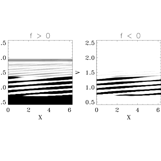
Figure 5: Quantum phase space portrait of the electron Wigner function in the region around the phase velocity of the wave. Position is normalized to $\lambda_{F}$ and velocity to $v_{F}$. Same parameters as in Fig. 4, with in addition $H=1$. Left frame: positive part of $f(x,v)$; right frame: negative part of $f$.

Figure 6: Time evolution of the potential energy, normalized to the Fermi energy, for the classical case (left frame) and the quantum case with $H=1$ (right frame).

6 Conclusions and future developments

In this paper, we have reviewed a number of kinetic and fluid models that are appropriate to study the behavior of collisionless plasmas when quantum effects are not negligible. The main application of these models concerns the dynamics of electrons in ordinary metals as well as metallic nanostructures (clusters, nanoparticles, thin films). In particular, it is now possible to study experimentally the electron dynamics on ultrafast (femtosecond) time scales that correspond to the typical collective plasma effects in the electron gas. The properties of a quantum electron plasma (neutralized by the background ions) can thus be measured with good accuracy and compared to the theoretical predictions.

The main drawback of the models described in this paper is that they all neglect electron-electron collisions. Strictly speaking, the collisionless approximation should be valid only when $g_{Q}\ll 1$, which is not true for electrons in metals (see Table 1). As we discussed in Sec. 3, Pauli blocking does reduce the effect of collisions for distributions near equilibrium, but many interesting phenomena involve nonequilibrium electrons, so that the validity of the collisionless approximation is not completely clear. It is possible, in principle, to include collisional effects in semiclassical models such as the Vlasov-Poisson system, by simply adding a collision operator on the right-hand side of the Vlasov equation [5]. The collision operator relevant for a degenerate fermion gas is known as the Ühling-Uhlenbeck collision term and is basically a Boltzmann collision operator that takes into account the exclusion principle. Even in the semiclassical case, however, the validity of the Ühling-Uhlenbeck approach may be questioned for strongly coupled plasmas ($g_{Q}\gtrsim 1$), for which it is conceptually difficult to separate the mean-field from the collisional effects.

It is much harder to include a simple collisional term in truly quantum models, such as the Wigner or Hartree equations [45]. There is a vast literature on dissipative quantum mechanics, but this is concerned with the interaction of a single quantum particle with an external environment [46, 47, 48]. In addition, the coupling to the environment is generally assumed to be weak, which is not the case for metallic electrons. Recent approaches to the dynamics of strongly coupled quantum plasmas range from quantum Monte Carlo methods (for the equilibrium) to quantum molecular dynamics simulations (for the nonequilibrium dynamics) [15, 49].

We shall mention another two possible extensions of the models presented in this paper, but these are more technical points, rather than conceptual issues such as the above-mentioned inclusion of electron-electron collisions in the strongly coupled regime.

The first issue concerns the coupling to the ion lattice. So far, we have assumed that the ions form a motionless positively-charged background described by the equilibrium density $n_{0}(x)$, which may be position-dependent for open systems such as clusters. This is appropriate for times shorter than the typical ion-electron collision time (see Table 1), but for longer times the ion dynamics must be taken into account. The ion dynamics, just like the electrons’, may be split into a mean-field part and a collisional part. If we want to include only the mean-field component (and neglect ion-electron collisions), then all we need to do is add a Vlasov equation for the ionic species, supplemented by a Maxwell-Boltzmann initial condition (as the ions are always classical) – see, for instance, [32]. This is conceptually simple, though it may require rather long simulation times, because the typical ionic time scale (proportional to $\omega_{pi}$) is much longer than the electrons’. As a first approximation, electron-ion collisions may be modelled by a simple relaxation term of the Bathnagar-Gross-Krook type [50], which is the kinetic analog of the Drude relaxation model of solid state physics [14]. For a more accurate approach that includes the full ion dynamics (mean-field and collisional), it will be necessary to treat the ions with molecular dynamics simulations.

Finally, one should consider the effect of magnetic fields (both external and self-consistent) on the plasma dynamics. Magnetic fields should not alter the main conclusions drawn in the present work and are easily included in all the equations presented here. For very strong fields, fusion and space plasma physicists have developed a battery of approximations (guiding-center, gyrokinetic, …) that allow one to reduce the complexity of the relevant models. It is a challenging task to transpose these methods to the physics of quantum plasmas [51, 52]. Magnetic fields should also trigger spin effects, which are uniquely quantum-mechanical. The interaction of spin and Coulomb effects, still a largely unexplored field, is thus likely to become an active area of future research.

Acknowledgments
I would like to thank Paul-Antoine Hervieux for his careful reading of the manuscript and useful suggestions.

References

- [1] F. Calvayrac, P.-G. Reinhard, E. Suraud, and C. Ullrich, Nonlinear electron dynamics in metal clusters. Phys. Rep. 337 (2000), 493–578.
- [2] S. D. Brorson, J. G. Fujimoto, and E. P. Ippen, Femtosecond electronic heat-transport dynamics in thin gold films. Phys. Rev. Lett. 59 (1987), 1962–1965.
- [3] C. Suárez, W. E. Bron, and T. Juhasz, Dynamics and transport of electronic carriers in thin gold films. Phys. Rev. Lett. 75 (1995), 4536–4539.
- [4] J.-Y. Bigot, V. Halté, J.-C. Merle, and A. Daunois, Electron dynamics in metallic nanoparticles. Chem. Phys. 251 (2000), 181–203.
- [5] A. Domps, P.-G. Reinhard, and E. Suraud, Fermionic Vlasov propagation for Coulomb interacting systems. Ann. Phys. (N.Y.) 260 (1997), 171–190.
- [6] N. C. Kluksdahl, A. M. Kriman, D. K. Ferry, and C. Ringhofer, Self-consistent study of the resonant-tunneling diode. Phys. Rev. B 39 (1989), 7720–7735.
- [7] P. A. Markowich, C. A. Ringhofer, and C. Schmeiser, Semiconductor equations, Springer, Vienna, 1990.
- [8] M. C. Yalabik, G. Neofotistos, K. Diff, H. Guo and J. D. Gunton, Quantum mechanical simulation of charge transport in very small semiconductor structures. IEEE Trans. Electron Devices 36 (1989), 1009–1013.
- [9] J. H. Luscombe, A. M. Bouchard and M. Luban, Electron confinement in quantum nanostructures: Self-consistent Poisson-Schrödinger theory. Phys. Rev. B 46 (1992), 10262–10268.
- [10] A. Arnold and H. Steinrück, The ‘electromagnetic’ Wigner equation for an electron with spin. Z. Angew. Math. Phys. 40 (1989), 793–815.
- [11] Shmuel Balberg and Stuart L. Shapiro, The properties of matter in white dwarfs and neutron stars, astro-ph/0004317.
- [12] F. F. Chen, Introduction to plasma physics and controlled fusion, Plenum Press, New York, 1984.
- [13] L. D. Landau and E. M. Lifshitz, Statistical Physics, part 1, Butterworth-Heinemann, Oxford, 1980.
- [14] N. W. Ashcroft and N. D. Mermin, Solid state physics, Saunders College Publishing, Orlando, 1976.
- [15] M. Bonitz et al., Theory and simulation of strong correlations in quantum Coulomb systems. J. Phys. A: Math. Gen. 36 (2003), 5921–5930.
- [16] E. P. Wigner, On the quantum correction for thermodynamic equilibrium. Phys. Rev. 40 (1932), 749–759.
- [17] J. E. Moyal, Quantum mechanics as a statistical theory. Proc. Cambridge Phil. Soc. 45 (1949), 99–124.
- [18] V. I. Tatarskii, The Wigner representation of quantum mechanics. Sov. Phys. Usp. 26 (1983), 311–327 [Usp. Fis. Nauk. 139 (1983), 587].
- [19] M. Hillery, R. F. O’Connell, M. O. Scully, and E. P. Wigner, Distribution functions in physics: Fundamentals. Phys. Rep. 106 (1984), 121–167.
- [20] G. Manfredi and M. R. Feix, Entropy and Wigner functions. Phys. Rev. E 53 (1996), 6460–6470.
- [21] J.E. Drummond, Plasma Physics, McGraw- Hill, New York, 1961.
- [22] F. Haas, G. Manfredi, J. Goedert, Nyquist method for Wigner-Poisson quantum plasmas. Phys. Rev. E 64 (2001), 026413.
- [23] M. Bonitz, D. C. Scott, R. Binder, and S. W. Scott, Nonlinear carrier-plasmon interaction in a one-dimensional quantum plasma. Phys. Rev. B 50 (1994), 15095–15098.
- [24] E. K. U. Gross, J. F. Dobson, and M. Petersilka, Density functional theory of time-dependent phenomena, Topics in Current Chemistry, vol. 181, Springer, Berlin, 1996, pp. 81-172.
- [25] D. Pines, Classical and quantum plasmas. J. Nucl. Energy C 2 (1961), 5-17.
- [26] J. Dawson, On Landau damping. Phys. Fluids 4 (1961), 869-874.
- [27] F. Haas, G. Manfredi and M. R. Feix, Multistream model for quantum plasmas. Phys. Rev. E 62 (2000), 2763–2772.
- [28] D. Anderson, B. Hall, M. Lisak, and M. Marklund, Statistical effects in the multistream model for quantum plasmas. Phys. Rev. E 65 (2002), 046417.
- [29] G. Manfredi and F. Haas, Self-consistent fluid model for a quantum electron gas. Phys. Rev. B 64 (2001), 075316.
- [30] I. Gasser, P. A. Markowich, and A. Unterreiter, in Modeling of collisions, edited by P.-A. Raviart, Gauthier-Villars, Paris, 1997.
- [31] C. L. Gardner, Quantum hydrodynamic model for semiconductor devices. SIAM J. Appl. Math. 54 (1994), 409–427.
- [32] G. Manfredi and P.-A. Hervieux, Vlasov simulations of ultrafast electron dynamics and transport in thin metal films. Phys. Rev. B 70 (2004), 201402(R).
- [33] W. R. Frensley, Boundary conditions for open quantum systems driven far from equilibrium. Rev. Mod. Phys. 62 (1990), 745–791.
- [34] W. Kohn and L. J. Sham, Self-consistent equations including exchange and correlation effects. Phys. Rev. 140 (1965), A1133–A1138.
- [35] W. Ekardt, Work function of small metal particles: Self-consistent spherical jellium-background model. Phys. Rev. B 29 (1984), 1558–1564.
- [36] R. G. Parr and W. Young, Density functional theory of atoms and molecules, Oxford University Press, New York, 1989.
- [37] R. Balescu, Statistical mechanics of charged particles, John Wiley, London, 1963.
- [38] M. Bonitz, R. Binder, D. C. Scott, S. W. Koch, and D. Kremp, Theory of plasmons in quasi-one-dimensional degenerate plasmas. Phys. Rev. E 49 (1994), 5535–5545.
- [39] P. Bertrand and M. R. Feix, Non linear electron plasma oscillation: the ”water bag model”. Phys. Lett. A 28 (1968), 68–69.
- [40] L. D. Landau, On the vibration of the electronic plasma. J. Phys. (Moskow) 10 (1946), 25.
- [41] N. Suh, M. R. Feix, and P. Bertrand, Numerical simulation of the quantum Liouville-Poisson system. J. Comput. Phys. 94 (1991), 403–418.
- [42] G. Manfredi, Long-time behavior of nonlinear landau damping. Phys. Rev. Lett. 79 (1997), 2815–2818.
- [43] C. Z. Cheng and G. Knorr, The integration of the Vlasov equation in configuration space. J. Comput. Phys. 22 (1976), 330–351.
- [44] F. Filbet, E. Sonnendrucker, and P. Bertrand, Conservative numerical schemes for the Vlasov equation. J. Comput. Phys. 172 (2001), 166–187.
- [45] J. L. Lopez, Nonlinear Ginzburg-Landau-type approach to quantum dissipation. Phys. Rev. E 69 (2004), 026110.
- [46] A. O. Caldeira and A. J. Leggett, Path integral approach to quantum Brownian motion. Physica A 121 (1983), 587–616.
- [47] L. Diosi, Calderia-Leggett master equation and medium temperatures. Physica A 199 (1993), 517–526.
- [48] W. H. Zurek, S. Habib, and J. P. Paz, Coherent states via decoherence. Phys. Rev. Lett. 70 (1993), 1187–1190.
- [49] W. Ebeling, A. Förstery, H. Hessz and M. Yu. Romanovsky, Thermodynamic and kinetic properties of hot nonideal plasmas. Plasma Phys. Control. Fusion 38 (1996), A31 -A47.
- [50] P. L. Bathnagar, E. P. Gross, and M. Krook, A model for collision processes in gases. I. Small amplitude processes in charged and neutral one-component systems. Phys. Rev. 94 (1954), 511–525.
- [51] B. Shokri and A. A. Rukhadze, Quantum surface wave on a thin plasma layer. Phys. Plasmas 6 (1999), 3450–3454.
- [52] B. Shokri and A. A. Rukhadze, Quantum drift waves. Phys. Plasmas 6 (1999), 4467–4471.