Solvable Quantum Two-body Problem: Entanglement

Abstract

A simple one dimensional model is introduced describing a two particle “atom” approaching a point at which the interaction between the particles is lost. The wave function is obtained analytically and analyzed to display the entangled nature of the subsequent state.

1 Introduction

The notion of entanglement was introduced by Schrödinger [1] who considered as the essential feature of quantum mechanics the fact that when two particles interact by a known force and then separate, they can no longer be considered as independent. This ought to be evident in the case of a hydrogenic atom for which, by some mechanism, the interparticle interaction is lost and the atom is ionized. The entangled nature of the state must be evident in the structure of the two-particle wave function, but this does not appear to have been examined in detail. The aim of this note is to study this situation for an exactly solvable two-particle system.

A suitable one dimensional model was introduced in [2] to describe the interaction of a hydrogenic atom with a “metal” surface, such that once the atom penetrates the metal the nuclear “charge” is screened to zero. It was found that the problem could be re-expressed as the Wiener-Hopf problem introduced in 1947 to describe the reflection of an electromagnetic wave from a linear coastline solved in 1952 by Bazer and Karp. Their work is reviewed in [3] and from the results, a formal expression for the two-body wave function was obtained along with an exact formula for the reflection coefficient as a function of the incident energy $E$.

In the atomic center of mass system (total mass $M$, center of mass coordinate $R$, reduced mass $\mu$ and relative coordinate $r$) the interaction potential for the model is $V(R,r)=-\lambda\delta(r)$ outside the metal ($R>0$) and 0 inside ($R<0$). In terms of reduced variables:

$$y=\sqrt{\mu/M}r,\ \ k_{0}^{2}=2ME/\hbar^{2},\ \ a=\sqrt{M\mu}\lambda/\hbar^{2},\ \ K^{2}=k_{0}^{2}+a^{2}$$ (1.1)

the wave function is (the sign in the exponent of the Fourier transform has been altered from that in [2] to reflect standard usage)

$$\psi(R,y) = \exp[-\rmi KR-a|y|]+\frac{a^{2}[\sigma^{+}(K)]^{2}}{2K^{2}}\exp[\rmi KR-a|y|]$$ (1.2)

$$-\frac{a\sigma^{+}(K)}{2\pi\rmi}\oint\frac{\exp[-\rmi kR-|y|\sqrt{k^{2}-k_{0}^{2}}]}{(k+K)[a-\sqrt{k^{2}-k_{0}^{2}}]}\ \sigma^{+}(k)\ \rmd k\quad(R>0),$$

$$\psi(R,y) = \frac{a\sigma^{+}(K)}{2\pi\rmi}\oint\frac{\exp[-\rmi kR-|y|\sqrt{k^{2}-k_{0}^{2}}]}{(k+K)\sqrt{k^{2}-k_{0}^{2}}}\ \sigma^{-}(k)\ \rmd k\quad(R<0),$$ (1.3)

where, $\sigma^{\pm}(k)$ are the Wiener-Hopf factors [4] of the kernel

$$\sigma(k)=1-\frac{a}{\sqrt{k^{2}-k_{0}^{2}}}=\frac{\sigma^{+}(k)}{\sigma^{-}(k)}$$ (1.4)

and the contours for the integrals in (1.2) and (1.3) surround branch cuts associated with $\pm k_{0}$ (which, for technical reasons, have infinitesimal imaginary parts) in the upper and lower half planes.

The leading term on the right hand side of (1.2) represents an incoming atom and is normalized to unit amplitude; the second term represents the atom reflected from the surface with reflection coefficient [2]

$${\cal{R}}=\frac{(K-k_{0})^{2}}{K^{2}}.$$ (1.5)

The task here is to analyze the integrals in (1.2) and (1.3) which describe the entanglement of the atomic particles in the “ionized” state. Since for $R<0$ there is no direct interaction between the two particles comprising the atom, a dependence of the wave function on the relative coordinate $y$ indicates the quantum entanglement of the two particles.

In the following section we change (1.3) and (1.4) into somewhat more convenient forms and express all the components of the Wiener-Hopf solution in terms of standard functions. In the concluding section details of the wave functions are presented and we find that indeed, even for $R$ large and negative, the two-particle wave function is not separable.

2 Calculation

We begin by investigating the Wiener-Hopf factorization of $\sigma(k)$ (1.4). Only the magnitude of the $+$ factor at the value $k=K$ was needed in [2]; we now require its complex value for ${\rm Im\;}k\geq 0$. The calculation is simplified somewhat by introducing the modified kernel

$$S(k)=\frac{k^{2}-k_{0}^{2}}{k^{2}-K^{2}}\ \sigma(k)=\frac{S_{+}(k)}{S_{-}(k)}$$ (2.1)

in terms of which (1.2) and (1.3) become

$$\psi(R,y)=\exp[-\rmi KR-a|y|]+2\left(\frac{K-k_{0}}{K+k_{0}}\right)S^{2}_{+}(K)\exp[\rmi KR-a|y|]-\Phi(R,y)$$ (2.2)

$$\Phi(R,y)=\frac{2aK}{K+k_{0}}S_{+}(K)\oint\frac{\rmd k}{2\pi\rmi}\ \sqrt{\frac{k+k_{0}}{k-k_{0}}}\ \frac{\exp[-\rmi kR-|y|\sqrt{k^{2}-k_{0}^{2}}]}{S_{+}(k)(K^{2}-k^{2})}\mbox{\hskip 14.45377pt}(R>0),$$ (2.3)

where the contour encloses the branch cut running from $-k_{0}$ in the lower half plane, parallel to the real axis to the imaginary axis and then to $-i\infty$. For $R<0$,

$$\psi(R,y)=\frac{2aKS_{+}(K)}{K+k_{0}}\oint\frac{\rmd k}{2\pi\rmi}\ \sqrt{\frac{k+k_{0}}{k-k_{0}}}\ \frac{\exp[-\rmi kR-|y|\sqrt{k^{2}-k_{0}^{2}}]}{S_{+}(k)(K^{2}-k^{2})}$$ (2.4)

where the contour surrounds the branch cut running from $k_{0}$, parallel to the real axis up to the imaginary axis and then to $i\infty$. An alternative derivation of (2.2)–(2.4) is outlined in Appendix A.

Now [3, 5],

$$S_{+}(k) = \exp[-J(k)]$$

$$J(k) = \frac{1}{2\pi\rmi}\int_{-\infty}^{\infty}{\rm Log}\left[1+\frac{a}{\sqrt{u^{2}-k_{0}^{2}}}\right]\frac{\rmd u}{u-k},$$ (2.5)

where the contour runs along the real axis indented below $u=k$. By breaking the range into $[-\infty,0]\cup[0,\infty]$ and combining the two integrals we have

$$J(k)=\frac{k}{\pi\rmi}\int_{0}^{\infty}{\rm Log}\left[1+\frac{a}{\sqrt{u^{2}-k_{0}^{2}}}\right]\ \frac{\rmd u}{u^{2}-k^{2}}.$$ (2.6)

Next, by letting $u\rightarrow-\rmi s$ and, since there are now no singularities in the first quadrant, rotating the contour back to the real axis, with $s\rightarrow ks$, we find

$$J(k) = \frac{1}{\pi}\int_{0}^{\infty}\frac{\rmd s}{s^{2}+1}{\rm Log}\left[1-\frac{\rmi a}{k\sqrt{s^{2}+(k_{0}/k)^{2}}}\right]$$ (2.7)

$$= \frac{1}{\pi}\int_{0}^{\infty}\frac{\rmd s}{s^{2}+1}{\rm Log}[\sqrt{s^{2}+(k_{0}/k)^{2}}-\rmi a/k]-\frac{1}{2\pi}\int_{0}^{\infty}\frac{{\rm Log}[s^{2}+(k_{0}/k)^{2}]}{s^{2}+1}\ \rmd s.$$

The second integral, as can be found in tables, is $\pi{\rm Log}[1+(k_{0}/k)]$; the first integral is evaluated in Appendix B yielding

$$S_{+}(k)=\sqrt{\frac{k+k_{0}}{k+K}}\ \exp\left[\frac{2\rmi}{\pi}\ {\rm Im\;Ti}_{2}\left(\frac{\sqrt{k_{0}^{2}-k^{2}}+\rmi a}{K+k}\right)\right].$$ (2.8)

where ${\rm Ti}_{2}(z)$ is the Arctangent integral function, defined in (2.3). Formula (2.8) is valid for ${\rm Im\;}k\geq 0$, except for $k=\pm K$, where there is a confluence of singularities. However, this case can be extracted from the results given in [2] whence we find

$$S_{+}(K)=\sqrt{\frac{K+k_{0}}{2K}}\ \exp\left[\frac{\rmi}{2\pi}\,\biggl{(}{\rm Li}_{2}(-a/K)-{\rm Li}_{2}(a/K)\biggr{)}\right].$$ (2.9)

$$S_{+}(K)S_{+}(-K)=\frac{1}{2}.$$ (2.10)

3 Results and conclusions

We turn now to the wave function (2.4) in the interaction-free region. At this point the imaginary part of $k_{0}$ can be set to zero and on the part of the contour surrounding the vertical portion of the branch cut, where the factor $\exp(-\rmi kR)$ is a decaying exponential, the contribution to the integral will be small and we shall neglect it. Similarly, since the contribution of the contour in the upper half plane about the interval $[0,k_{0}]$ is exponentially small compared to the part in the lower half plane, for $R<0$ we have

$$\psi(R,y)\approx\frac{2aK}{K+k_{0}}S_{+}(K)\int_{0}^{k_{0}}\frac{\rmd k}{2\pi}\ \sqrt{\frac{k_{0}+k}{k_{0}-k}}\ \frac{\exp[-\rmi kR-\rmi|y|\sqrt{k_{0}^{2}-k^{2}}]}{S_{+}(k)(K^{2}-k^{2})}.$$ (3.1)

Note that, from (1.5), as $k_{0}\to 0$, ${\cal{R}}=1$ signifying total reflection. Accordingly, from (3.1), $|\psi(R,y)|^{2}=0$ apart from a rapidly decaying evanescent wave due to the neglected part of the contour.

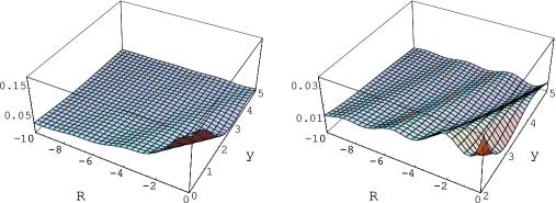
Figure 1: Square of the wave function amplitude $|\psi(R,y)|^{2}$: $a=1$, $k_{0}=2$

We have evaluated (3.1) numerically for $a=1$, $k_{0}=2$, and present the square of its amplitude as a function of $|y|$ and $|R|$ for $a=1$ and $k_{0}=2$ in Fig. 1. In Fig. 2 we show the real and imaginary parts of $\psi(R,y)$. For $R$ large and negative, but $|y|\ll|R|$, the integral can be estimated by setting $k=0$ in the integrand, apart from the factor $\exp(-ikR)$, leading to

$$\psi(R,y)\approx\frac{a}{\rmi\pi K^{2}R\sqrt{2k_{0}(K+k_{0})}}\ e^{-\rmi[k_{0}|y|+\phi_{-}]}$$ (3.2)

$$\phi_{-}=\frac{2}{\pi}\ {\rm Im\;Ti}_{2}\left(\frac{k_{0}+\rmi a}{K}\right).$$

Thus, the amplitude decays as $|R|^{-1}$ and even far away from the point where the particles are decoupled, the relative coordinate is present in the phase. For larger values of $|y|$, the amplitude appears to be ${\rm o}(|y|^{-3/4})$ and oscillates as $y\to\infty$, which is illustrated in Fig. 3 showing $|\psi(-10,y)|^{2}$ for $a=1$, $k_{0}=2$.

A natural quantity to examine is the expected value

$$Y(R)=\frac{\int_{-\infty}^{\infty}|y||\psi(R,y)|^{2}\rmd y}{\int_{-\infty}^{\infty}|\psi(R,y)|^{2}\rmd y}$$ (3.3)

of the relative particle displacement . Our numerical integration of the numerator in( 3.3) appears to diverge in the interaction-free region $R<0$. To obtain a reliable result will require a more detailed asymptotic study of the wave function for $|y|/R\rightarrow\infty$. Finally, in Figure 4 we show the square amplitude of the wave function (1.2) for $R>0$ with $a=1$ and $k_{0}=2$ (including the incident wave).

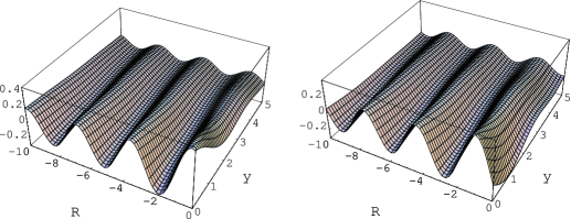
Figure 2: Real (left) and Imaginary (right) parts of $\psi(R,y)$: $a=1$, $k_{0}=2$

For $R\gg 1$ the integral in (1.3) has been treated by Kay [3] who used the method of steepest descent. From his results we find for the integral in (2.3),

$$\Phi(R,y)\approx\frac{\rmi^{3/2}k_{0}a}{4\pi^{1/2}(k_{0}R)^{1/2}}\frac{\xi^{2}}{a^{2}+K^{2}\xi^{2}}\sqrt{\frac{k_{0}}{K}\frac{K+k_{0}}{K+\frac{1}{2}k_{0}\xi^{2}}}\ e^{\rmi[k_{0}R(1-\frac{1}{2}\xi^{2})+\frac{2}{\pi}\phi_{+}]}$$ (3.4)

$$\phi_{+}=\frac{1}{2}\,{\rm Li}_{2}(a^{2}/K^{2})-2{\rm Li}_{2}(a/K)-{\rm Im\;Ti}_{2}\left(\frac{k_{0}\xi+\rmi a}{K-k_{0}+\frac{1}{2}k_{0}\xi^{2}}\right)$$

where $\xi=y/R<1$. This represents an outgoing wave with no trace of the factor $\exp(-a|y|)$ representing the atomic state.

Figure 3: $|\psi(-10,y)|^{2}$: $a=1$, $k_{0}=2$

Figure 4: $|\psi(R,0)|^{2}$ (upper curve) and $|\psi(R,.5)|^{2}$ for $R>0$: $a=1$, $k_{0}=2$

Appendix A

The two-particle Schrödinger equation is

$$L\psi(R,y)=V(R,y)\psi(R,y)$$ (1.1)

where $L=\partial_{R}^{2}+\partial_{y}^{2}+k_{0}^{2}$ and has the Green function $G(R-R^{\prime},y-y^{\prime};k_{0})$, which in momentum space is simply $[P_{R}^{2}+p_{y}^{2}-k_{0}^{2}]^{-1}$

The solution of (1.1) is

$$\psi(R,y)=\int_{-\infty}^{\infty}\int_{-\infty}^{\infty}G(R-R^{\prime}y-y^{\prime};k_{0})V(R^{\prime},y^{\prime})\psi(R^{\prime},y^{\prime})\ \rmd R^{\prime}\,\rmd y^{\prime}.$$

In terms of $h(R)=\psi(R,0)$ this reduces to

$$\psi(R,y)=2a\int_{0}^{\infty}G(R-R^{\prime},y;k_{0})h(R^{\prime})\,\rmd R^{\prime}$$ (1.2)

and, in particular,

$$h_{+}(R)+h_{-}(R)=2a\int_{-\infty}^{\infty}G(R-R^{\prime},0;k_{0})h_{+}(R^{\prime})\,\rmd R^{\prime}$$ (1.3)

where $h_{+}(R)=h(R)\Theta(R)$, $h_{-}(R)=h(R)\Theta(-R)$. The Fourier transforms of these functions $H_{+}(k)$ and $H_{-}(k)$ are analytic in the upper and lower half $k$-plane, respectively. Since the integral in (1.3) is a convolution, by taking the Fourier transform (1.3) becomes

$$H_{+}(k)+H_{-}(k)=2ag_{0}(k)H_{+}(k)$$ (1.4)

where $g_{0}(k)=1/2\sqrt{k^{2}-k_{0}^{2}}$ is the Fourier transform of $G(R,0;k_{0})$. Therefore,

$$\frac{H_{-}(k)}{H_{+}(k)}=\frac{k^{2}-K^{2}}{k^{2}-k_{0}^{2}}S(k)$$ (1.5)

where

$$S(k)=\frac{k^{2}-k_{0}^{2}-a\sqrt{k^{2}-k_{0}^{2}}}{k^{2}-K^{2}}=\frac{S_{+}(k)}{S_{-}(k)}$$ (1.6)

and $S_{+}(k)(S_{-}(k))$ is analytic and free of zeros for ${\rm Im\;}k>0$ (${\rm Im\;}k<0$). Equation (1.6) implies that $(k^{2}-K^{2})S_{+}(k)H_{+}(k)/(k+k_{0})$ is a bounded entire function and is therefore a constant $\alpha$. Consequently,

$$h_{+}(R)=\frac{\alpha}{2\pi}\int_{-\infty+\rmi c}^{\infty+\rmi c}\frac{k+k_{0}}{S_{+}(k)(k^{2}-K^{2})}\ e^{-\rmi kR}\ \rmd k$$ (1.7)

with ${\rm Im\;}K<c<{\rm Im\;}k_{0}$. Thus, we have from (1.2), for $-\infty<R<\infty$,

$$\psi(R,y)=\frac{a\alpha}{2\pi\rmi}\int_{-\infty+\rmi c}^{\infty+\rmi c}\rmd k\ \sqrt{\frac{k_{0}+k}{k_{0}-k}}\ \frac{e^{-\rmi kR-|y|\sqrt{k^{2}-k_{0}^{2}}}}{(k^{2}-K^{2})S_{+}(k)}.$$ (1.8)

For $R>0$ the contour can be closed into the lower half plane, which contains the two poles $\pm K$ and the branch point $-k_{0}$ yielding (2.2)–(2.3), while for $R<0$ the contour can be closed into the upper half plane yielding (2.4).

Appendix B

Here we evaluate the integral

$$\int_{0}^{\infty}\frac{{\rm Log}[\sqrt{x^{2}+c^{2}}+d]}{x^{2}+1}\ \rmd x$$ (2.1)

needed to obtain $S_{+}(k)$. We begin indirectly by setting

$$A=\frac{y\cot(\theta/2)}{1+\sqrt{y^{2}+1}}\mbox{ \hskip 14.45377pt}B=\frac{y\tan(\theta/2)}{1+\sqrt{1+y^{2}}}.$$ (2.2)

Then

$$\frac{A+B}{1-AB}=y\csc(\theta)$$

and

$$\tan^{-1}(y\csc(\theta))=\tan^{-1}(A)+\tan^{-1}(B).$$

But,

$$\csc(\theta)\tan^{-1}(y\csc(\theta))=-\frac{d}{d\theta}\int_{1}^{\csc(\theta)}\frac{\tan^{-1}(yu)}{\sqrt{u^{2}-1}}\ \rmd u$$

$$\csc(\theta)\tan^{-1}(A)=-\frac{d}{d\theta}\int_{0}^{A}\frac{\tan^{-1}(u)}{u}\ \rmd u$$

$$\csc(\theta)\tan^{-1}(B)=\frac{d}{d\theta}\int_{0}^{B}\frac{\tan^{-1}(u)}{u}\ \rmd u.$$

Therefore,

$$\int_{1}^{\csc(\theta)}\frac{\tan^{-1}(yu)}{\sqrt{u^{2}-1}}\ \rmd u={\rm Ti}_{2}(A)-{\rm Ti}_{2}(B)+C,$$

where

$${\rm Ti}_{2}(z)=\int_{0}^{z}\frac{\tan^{-1}(u)}{u}\ \rmd u$$ (2.3)

is the Arctangent integral function and $C$ is independent of $\theta$. However, for $\theta=\pi/2$, $A=B$ and the LHS vanishes, so $C=0$. Now set

$$\theta=\csc^{-1}\sqrt{\frac{b^{2}-a^{2}+1}{1-a^{2}}},\mbox{\hskip 14.45377pt}y=\sqrt{1-a^{-2}}\mbox{\hskip 7.22743ptand\hskip 7.22743pt}u=\sqrt{\frac{x^{2}-a^{2}+1}{1-a^{2}}}.$$

This gives

$$\int_{0}^{b}\frac{\rmd x}{\sqrt{x^{2}+1-a^{2}}}\tan^{-1}\left(\frac{\sqrt{x^{2}+1-a^{2}}}{a}\right)=$$

$${\rm Ti}_{2}\left(\frac{\sqrt{b^{2}+1-a^{2}}+b}{1+a}\right)-{\rm Ti}_{2}\left(\frac{\sqrt{b^{2}+1-a^{2}}-b}{1+a}\right).$$ (2.4)

We next define

$$g(a,b)=\int_{0}^{\infty}\frac{\rmd s}{s^{2}+1}{\rm Log}[\sqrt{b^{2}(s^{2}+1)+1}+a].$$

Then $g(a,0)=(\pi/2){\rm Log}(1+a)$ and

$$\frac{\partial}{\partial b}g(a,b)=b\int_{0}^{\infty}\frac{[\sqrt{b^{2}(s^{2}+1)+1}-a]\ \rmd u}{(b^{2}s^{2}+b^{2}+1-a^{2})\sqrt{b^{2}(s^{2}+1)+1}}=\frac{\tan^{-1}(\sqrt{b^{2}+1-a^{2}}/a)}{\sqrt{b^{2}+1-a^{2}}}.$$

Reintegration using (2.4) gives

$$g(a,b)=\frac{\pi}{2}\ln(1+a)+{\rm Ti}_{2}\left(\frac{\sqrt{b^{2}+1-a^{2}}+b}{1+a}\right)-{\rm Ti}_{2}\left(\frac{\sqrt{b^{2}+1-a^{2}}-b}{1+a}\right),$$

which is easily transformed into

$$\int_{0}^{\infty}\frac{{\rm Log}[\sqrt{x^{2}+c^{2}}+\alpha]}{x^{2}+1}\ \rmd x = \frac{\pi}{2}{\rm Log}[1+\sqrt{c^{2}-\alpha^{2}}]$$

$$+{\rm Ti}_{2}\left[\frac{\sqrt{c^{2}-1}+\alpha}{\sqrt{c^{2}-\alpha^{2}}+1}\right]+{\rm Ti}_{2}\left[\frac{\alpha-\sqrt{c^{2}-1}}{1+\sqrt{c^{2}-\alpha^{2}}}\right].$$

References

References

- [1] Schrödinger 1936 Proc. Camb. Phil. Soc. 31 555
- [2] Glasser M L 1993 J. Phys. A: Math. Gen. 26, L825
- [3] Bazer J and Karp S N 1962 J. Res. of the NBS-D. Radio Propagation 66D, 319
- [4] Karp S N 1950 Comm. Pure Appl. Math. 3, 411
- [5] Noble B 1958 The Wiener-Hopf technique (Pergamon Press, New York)