Quadratic pseudosupersymmetry in two-level systems

Abstract

Using the intertwining relation we construct a pseudosuperpartner for a (non-Hermitian) Dirac-like Hamiltonian describing a two-level system interacting in the rotating wave approximation with the electric component of an electromagnetic field. The two pseudosuperpartners and pseudosupersymmetry generators close a quadratic pseudosuperalgebra. A class of time dependent electric fields for which the equation of motion for a two level system placed in this field can be solved exactly is obtained. New interesting phenomenon is observed. There exists such a time-dependent detuning of the field frequency from the resonance value that the probability to populate the excited level ceases to oscillate and becomes a monotonically growing function of time tending to $3/4$. It is shown that near this fixed excitation regime the probability exhibits two kinds of oscillations. The oscillations with a small amplitude and a frequency close to the Rabi frequency (fast oscillations) take place at the background of the ones with a big amplitude and a small frequency (slow oscillations). During the period of slow oscillations the minimal value of the probability to populate the excited level may exceed $1/2$ suggesting for an ensemble of such two-level atoms the possibility to acquire the inverse population and exhibit lasing properties.

Corresponding Author: B F Samsonov

E-mail: samsonov@phys.tsu.ru

1 Introduction

The supersymmetry in physics has been introduced in the quantum field theory for unifying different interactions in a unique construct [1]. Supersymmetric formulation of quantum mechanics is due to the problem of spontaneous supersymmetry breaking [2]. Ideas of supersymmetry have been profitably applied to many nonrelativistic quantum mechanical problems since, and now there are no doubts that the supersymmetric quantum mechanics (SUSY QM) has its own right to exist (for recent developments see a special issue of Journal of Physics A, vol. 34, No 43, 2004). It is worth noticing that most papers in this field deal with the Hermitian Hamiltonians.

Differential equation of Schrödinger-like type with a non-Hermitian Hamiltonian appears in many physical models. One can cite quantum systems coupled to the environment like a hydrogen “atom” in an interacting medium subject to a dissipative force [3] (see also [4]) or different decay or collision reactions (see e. g. [5]; for more recent developments see [6]; in [7] the method of SUSY QM is involved). Physical needs initiated a deep mathematical study of spectral problems with non-Hermitian Hamiltonians in 50th and 60th of the previous century. The most essential result was first obtained by Keldysh [8] who proved the completeness of the set of eigenfunctions and associated functions for a regular Sturm-Liouville problem with a non-Hermitian Hamiltonian. In the books by Naimark [9] and Marchenko [10] one can find good reviews of these studies.

A new impact to studying different properties of non-Hermitian Hamiltonians is due to the discovery that the real character of the spectrum of a non-Hermitian Hamiltonian may be in particular related with so-called $\cal PT$-symmetry [11] and suggestion to generalize the quantum mechanics by accepting non-Hermitian Hamiltonians with a real spectrum to describe physical observables [12] (see also the review [13]). The necessary condition for such a generalization consists in the possibility to define a Hilbert space with a positive definite metric which is intimately related with the property of a Hamiltonian to be diagonalizable (for recent discussions see e.g. [14, 15]). This apparently may be assured in many cases since non-diagonalizable Hamiltonians may be transformed into diagonalizable ones by SUSY transformations [16]. The latter property permits us to suppose that the method of SUSY QM may become an essential ingredient of the complex quantum mechanics. This conjecture is also supported by established properties of this method not only to offer possibility for obtaining new exactly solvable complex potentials from known ones [17] but also to help deeper understanding different properties of complex potentials [17, 18]. In particular, an explicit construction of a superalgebra involving non-Hermitian Hamiltonians, which may be useful in different contexts i.e. integrability, quantization, different quantum field models etc, is shown to be possible [19] and even is now developed till the notion of pseudosupersymmetry [20] and nonlinear pseudosupersymmetry [21].

The relation of the general two-level model described by a non-Hermitian Hamiltonian acting in the two-dimensional Hilbert space $\mathbb{C}^{2}$ with the pseudosupersymmetry is discussed by Mostafazadeh [20]. In contrast to the approach of this author we reduce the time-dependent Schrödinger equation for the two level system, interacting in the rotating wave approximation with the electric component of an electromagnetic field, with a Hermitian Hamiltonian (see e.g. [22]) to the one-dimensional stationary Dirac equation with an effective non-Hermitian Hamiltonian where the time plays the role of the space variable. If we considered the spectral properties of the latter Hamiltonian we would define it in the Hilbert space $L^{2}(0,T)\otimes\mathbb{C}^{2}$. But as we shall see in our approach the spectral parameter in the Dirac equation is not related with spectral properties of the two-level system. Therefore we will not discuss any spectral features of this Hamiltonian and in particular its diagonalizability. Of course, the obtained Dirac equation is completely equivalent to the initial Schrödinger equation and if one studied it by usual means one would not get any new information about the two-level system. From this point of view the method of SUSY QM we are using proves its extreme efficiency once again.

To find a pseudosuperpartner for the given Dirac-like Hamiltonian we are using the technique of intertwining operators developed in [23] for the one-dimensional stationary Dirac equation. We have to notice that the application of results of this paper to our particular problem is not straightforward since transformation operators of the general form do not preserve the very peculiar form of the effective Dirac Hamiltonian corresponding to the two-level system. So, below we show how from the wide variety of possible transformations one can choose the necessary ones. In our approach in contrast to [20] the two pseudosuperpartners and pseudosupersymmetry generators constructed with the help of first order intertwiners close a quadratic pseudosuperalgebra. As it usually happens for the method of intertwining operators [24] if one of the two Hamiltonians is exactly solvable the same property takes place for the other. In this way starting from the simplest case corresponding to the famous Rabi oscillations we have found new electric fields having time-dependent frequencies for which the equation of motion of the two-level system has exact solutions. While analyzing solutions of the Schrödinger equation we have found a new interesting physical phenomenon. We show that there exists such a time-dependent detuning of the field frequency from the resonance value that the probability to populate the excited level ceases to oscillate and becomes a monotonically growing function of time tending to $3/4$. Of course this is a strictly fixed excitation regime similar to resonance. We also study how the above probability behaves under small deviations from this specific regime. We have found that when the parameters of the model are close enough to the specific values the probability exhibits two kinds of oscillations. The oscillations with a small amplitude and a frequency close to the Rabi frequency (fast oscillations) take place at the background of the ones with a big amplitude and a small frequency (slow oscillations). During the period of slow oscillations, which grows when the parameters of the model approach the above specific values, the minimal value of the probability to populate the excited level may exceed $1/2$ suggesting for an ensemble of such two-level atoms the possibility to acquire the inverse population and exhibit lasing properties.

We have to notice that some of the results we expose below are known from the previous paper [25]. These authors also use a similar intertwining technique but they do not relate it with the pseudosupersymmetry and do not give any analysis of solutions this method can provide with. Moreover, we give a deeper analysis of restrictions imposed on transformation operators by the features of the two-level system. In particular, we show that both the new Hamiltonian and solutions of the new Dirac equation can be expressed in terms of a real-valued function which is a solution of a second order differential equation with real coefficients. Since such equations have real solutions always our analysis opens the direct possibility to realize chains of transformations preserving the form of the Dirac-like Hamiltonian imposed by the features of the two-level system.

2 Preliminary

The two-level model in the rotating wave approximation with a possibly time-dependent detuning is described by the following system of equations (see e.g. [22]):

$$i\dot{A}_{1}-fA_{1}=\xi A_{2}\qquad i\dot{A}_{2}+fA_{2}=\xi A_{1}$$ (1)

where $\xi=\frac{1}{2\hbar}E_{0}d_{12}$, $d_{12}$ is the matrix element of the dipole interaction operator, $E_{0}$ is the amplitude of the electric component of an external electromagnetic field; $f=\frac{1}{2}\frac{d}{dt}(\delta t)$, $\delta(t)=\omega_{12}-\omega(t)$, $\omega_{12}=\frac{1}{\hbar}(\varepsilon_{1}-\varepsilon_{2})$, $\varepsilon_{1}$ and $\varepsilon_{2}$ are energy levels of the free atom and $\omega(t)$ is the field frequency; the dot over the symbol means the derivative with respect to time. While normalized properly the functions $|A_{1}(t)|^{2}$ and $|A_{2}(t)|^{2}$ give occupation probabilities for the ground and excited states respectively. If $\omega$ does not depend on time (hence $f=\frac{1}{2}\delta=\mbox{const}$) solutions of the system (1) are well-known. For instance, with the initial condition $A_{2}=0$ and $A_{1}=1$ at $t=0$ we get the well-known formula [22] for the excited state occupation probability if initially the system is in the ground state

$$P(t)=|A_{2}(t)|^{2}=\frac{\xi^{2}}{2\Omega^{2}}\left[1-\cos(2\Omega t)\right]\qquad\Omega^{2}=f^{2}+\xi^{2}$$ (2)

with $2\xi$ known as the Rabi frequency. The probability (2) is an oscillating function of time (so called Rabi oscillations). At the resonance ($f=\frac{1}{2}\delta=0$) it oscillates with the Rabi frequency. Therefore the value $\delta(t)$ characterizes the detuning of $\omega(t)$ from its resonance value equal $\omega_{12}$. In Section 5 using the formalism developed in Section 4 we shall get time-dependent functions $f=f(t)$ (and hence $\delta(t)$) for which system (1) permits exact solutions. As we show below (Section 5) time-dependent corrections to the detuning that we will consider although may change crucially the time-dependent behavior of the solutions of system (1) but they essentially keep oscillating character of the probability to populate the excited level with the frequency close to $2\Omega$. Yet, the absence of the Rabi oscillations may be considered as oscillations with the same frequency but with the zero amplitude since they may be obtained as corresponding limiting case of oscillations with a non-zero amplitude. So, in our approach the rotating wave approximation is as good as it is in the classical case of the electric field of a constant frequency.

Let us rewrite system (1) in the matrix form

$$h_{0}\Psi=E\Psi\qquad h_{0}=\gamma\partial_{t}+V_{0}$$ (3)

where

$$V_{0}=if_{0}\sigma_{y}$$ (4)

$\gamma=i\sigma_{x}$, $E=\xi$, $\Psi=(A_{1},A_{2})^{T}$ (the superscript “$T$” denotes the transposition) and we replaced $f$ (which we will call the “potential”) in (1) by $f_{0}$; $\sigma_{x,y,z}$ denote the standard Pauli matrices. Equation (3) is the one-dimensional stationary Dirac equation with the non-Hermitian Hamiltonian $h_{0}$ defined by the potential (4) where $t$ plays the role of the space variable. By construction the parameters $f_{0}$ and $E$ are real. For a fixed value of the dipole momentum of the irradiated system the parameter $E=\xi$ is defined by the amplitude of the electric field and, hence, is not related with spectral properties of the system. A useful comment is that since the Hamiltonian of the system (1) is Hermitian, $H_{sch}=\left(\begin{array}[]{cc}f&\xi\\ \xi&-f\end{array}\right)$, the evolution of the two-level system is unitary even for a time-dependent function $f=f(t)$. This means that the $\mathbb{C}^{2}$ inner product, $|A_{1}(t)|^{2}+|A_{2}(t)|^{2}$, for the Dirac equation (3) is $t$-independent.

3 SUSY algebra with non-Hermitian Hamiltonians

Let us have a non-Hermitian Hamiltonian $h_{0}$. We will not consider it as a Hamiltonian acting in a Hilbert space but to construct a SUSY algebra we need adjoint operators which we will introduce in a formal way. Denote by $h_{0}^{+}$ the operator formally adjoint to $h_{0}$. As usual the adjoint operation consists in taking the complex conjugation and transposition, the operator of the first derivative is skew-Hermitian and $(AB)^{+}=B^{+}A^{+}$.

Let $h_{1}$ be a “transformed Hamiltonian” which should be found together with the transformation operator $L$ by solving the intertwining relation $Lh_{0}=h_{1}L$ and $h_{1}^{+}$ be its adjoint. The later participates in the adjoint intertwining relation $h_{0}^{+}L^{+}=L^{+}h_{1}^{+}$. It means that the operator $L^{+}$ transforms eigenfunctions of $h_{1}^{+}$ into eigenfunctions of $h_{0}^{+}$.

Let us suppose that there exists an operator $J$ such that $h_{0,1}^{+}=Jh_{0,1}J$ and $J^{2}=\pm 1$, $J^{+}=\pm J$ (in general both signs may be accepted). Then from the adjoint intertwining relation it follows that $JL^{+}Jh_{1}=h_{0}JL^{+}J$ meaning that the operator $JL^{+}J$ realizes the backward transformation from $h_{1}$ to $h_{0}$ and the operator $JLJ$ transforms from $h_{0}^{+}$ to $h_{1}^{+}$. From here we infer that the superposition $JL^{+}JL$ transforms solutions of the equation (3) into solutions of the same equation meaning that this is a symmetry operator for this equation. In the simplest case when $L$ is a differential operator that we would like to consider this symmetry operator may be a function of $h_{0}$, so we will suppose that $JL^{+}JL=F_{1}(h_{0})$. By the same reason the superposition $LJL^{+}J$ may be a function of $h_{1}$ leading to $LJL^{+}J=F_{2}(h_{1})$. Moreover, we will also suppose that $F_{2}(x)=F_{1}(x)\equiv F(x)$ is an analytic function. These properties generalize the known factorization (polynomial factorization if $F(x)$ is a polynomial, see e.g. [23, 24]) properties taking place for the Hermitian case.

It follows from (3) and (4) that in our case $J=\sigma_{x}$.

Keeping in mind the properties of the operators $L$ and $J$ let us introduce the following matrix operators:

$$H=\left(\begin{array}[]{cc}h_{0}&0\\ 0&h_{1}\end{array}\right)\qquad Q_{1}=\left(\begin{array}[]{cc}0&0\\ L&0\end{array}\right)\qquad Q_{2}=\left(\begin{array}[]{cc}0&JL^{+}J\\ 0&0\end{array}\right).$$ (5)

It follows from the intertwining relations that the operators $Q_{1}$ and $Q_{2}$ commute with $H$ and they apparently are nilpotent. The above factorization properties are equivalent to the following anticommutation relation: $Q_{1}Q_{2}+Q_{2}Q_{1}=F(H)$.

Now if we identify our $J$ operator with $\eta_{-}=\eta_{+}^{-1}$ introduced in [20], $J=\eta_{-}=\eta_{+}^{-1}$, our $L$ operator with $D$ and $JL^{+}J$ with $D^{\sharp}$, we conclude that the operator $Q_{2}$ becomes pseudoadjoint to $Q_{1}$, the operators $H$,$Q_{1}$ and $Q_{2}$ close a nonlinear superalgebra and one can associate a nonlinear pseudosupersymmetry with quantum system described by the Hamiltonian $H$. In the next Section we shall show that a quadratic pseudosupersymmetry may be associated with the two-level system.

4 Intertwining operators for two-level Hamiltonians

To be able to associate a pseudosupersymmetry with the Hamiltonian given in (3) and (4) we have to find an intertwining operator and a partner Hamiltonian $h_{1}$. According to Ref. [23] the intertwining operator $L$ for a matrix equation such as (3) is defined with the help of a matrix-valued function ${\cal U}={\cal U}(t)$ satisfying the equation

$$h_{0}{\cal U}={\cal U}\Lambda\qquad\Lambda=\mbox{diag}(\lambda_{1},\lambda_{2})$$ (6)

called the “transformation function”, as follows:

$$L=\partial_{t}-W\qquad W=\dot{\cal U}{\cal U}^{-1}\,.$$ (7)

Here $\lambda_{1}$ and $\lambda_{2}$ are arbitrary constants. The operator $L$ transforms a solution $\Psi$ of equation (3) into a solution $\Phi$ of the same equation where the matrix $V_{0}$ is replaced by

$$V_{1}=V_{0}+\Delta V\qquad\Delta V=\gamma W-W\gamma\,.$$ (8)

Here and in the following the subscript $0$ marks quantities before the transformation and $1$ marks these after the transformation. It is not difficult to see that to preserve the form (4) of the potential so that $V_{1}=if_{1}\sigma_{y}$ it is sufficient to take the transformation function of the form

$${\cal U}=\left(\begin{array}[]{cc}u_{11}&u_{11}\\ u_{21}&-u_{21}\end{array}\right).$$ (9)

In this case the column-vector $U_{1}=(u_{11},u_{21})^{T}$ is a solution to the initial equation (3) corresponding to the eigenvalue $\lambda$ and the column-vector $U_{2}=(u_{11},-u_{21})^{T}$ is a solution to the same equation with the eigenvalue $-\lambda$ (note that this symmetry is built into the system (3)!) so that $\Lambda$ in (6) has the form $\Lambda=\mbox{diag}(\lambda,-\lambda)$. After some simple algebra one finds from (8) that $f_{1}=f_{0}+\Delta f$ where

$$\Delta f=\lambda\left(\frac{u_{11}}{u_{21}}-\frac{u_{21}}{u_{11}}\right)-2f_{0}\,.$$ (10)

In general, solutions $U_{1,2}$ of equation (3) from which the matrix ${\cal U}$ is composed, ${\cal U}=(U_{1},U_{2})$, are complex, leading to a complex-valued potential difference $\Delta f$. For physical reasons we require real potentials. A necessary condition for $\Delta f$ to be real is that the eigenvalue $\lambda$ be purely imaginary. Indeed, it is easy to show that $\lambda$ cannot be real. According to (10) $\Delta f$ is defined by the expression $\frac{u_{11\vphantom{I_{i}}}}{u_{21}}-\frac{u_{21\vphantom{I_{i}}}}{u_{11}}$. Putting $\frac{u_{11\vphantom{I_{i}}}}{u_{21}}=\varrho\exp(i\varphi)$ one finds

$$\frac{u_{11}}{u_{21}}-\frac{u_{21}}{u_{11}}=(\varrho-\frac{1}{\varrho})\cos\varphi+i(\varrho+\frac{1}{\varrho})\sin\varphi$$ (11)

and our claim follows from the fact that $\varrho+\frac{1}{\varrho}$ is never equal to zero. Finally one can prove that $\lambda^{2}$ is real (cf. [25]).

Now when the imaginary character of $\lambda$ is established we see from (10) that the left hand side of (11) must be purely imaginary, which is possible only if $\varrho=1$, meaning that $u_{11}$ and $u_{21}$ have the same absolute value. Therefore one can put $u_{11}=\rho\exp(i\varphi_{1})$ and $u_{21}=\rho\exp(i\varphi_{2})$. Using the fact that $U_{1}=(u_{11},u_{21})^{T}$ satisfies equation (3) with $E=\lambda$ and setting $\lambda=iR$, where $R$ is real, one gets from (3) a system of equations for $\rho$, $\varphi_{1}$ and $\varphi_{2}$. Of these equations we need only

$$\dot{\varphi}_{2}-\dot{\varphi}_{1}-2f_{0}+2R\sin(\varphi_{2}-\varphi_{1})=0\,.$$ (12)

If $R=0$ (12) can be readily integrated. Suppose $R\neq 0$. The change of the dependent variable in equation (12), $\varphi_{2}-\varphi_{1}=2\arctan q$, yields for $q$ the Riccati equation

$$\dot{q}+2Rq-f_{0}(1+q^{2})=0\,.$$ (13)

If $f_{0}=0$ the equation for $q$ is readily integrated: $q=\exp(-2Rt)$. Considering $f_{0}\neq 0$ one can linearize (13) by putting $q=-{\dot{u}}/({uf_{0}})$, so $u$ is a solution to the second order equation

$$\ddot{u}+(2R-{\dot{f}_{0}}/{f_{0}})\dot{u}+f_{0}^{2}u=0\,.$$ (14)

Introducing the new variable $\psi$ by putting $u=\exp(-Rt)\sqrt{f_{0}}\psi$ one eliminates the first derivative term from (14) thus obtaining

$$\ddot{\psi}+\left[f_{0}^{2}+\frac{1}{2}\frac{d^{2}}{dt^{2}}{\ln}f_{0}-\left(\frac{1}{2}\frac{d}{dt}\ln f_{0}-R\right)^{2}\right]\psi=0\,.$$ (15)

This equation has two linearly independent real solutions and, hence, $\psi$ is defined up to one real constant. Once $\psi$ is fixed one calculates $q$:

$$q=\frac{R}{f_{0}}-\frac{\dot{f}_{0}}{2f^{2}_{0}}-\frac{\dot{\psi}}{f_{0}\psi}$$ (16)

and the potential difference $\Delta f=2R\sin(\varphi_{2}-\varphi_{1})-2f_{0}$:

$$\Delta f=\frac{4Rq}{1+q^{2}}-2f_{0}\,.$$ (17)

Solution $\Phi$ of the equation $h_{1}\Phi=E\Phi$ with $h_{1}=\gamma\partial_{t}+V_{1}$, $V_{1}=V_{0}+\Delta V$, $\Delta V=i\Delta f\sigma_{y}$ can be found by applying the transformation operator (7) to solution $\Psi$ of the equation (3), $\Phi=L\Psi$. It is easy to see that the matrix $W$ is diagonal

$$W=\mbox{diag}\left(w_{1},w_{2}\right)\qquad w_{1}=-if_{0}+Ru_{21}/u_{11}\qquad w_{2}=w_{1}^{*}\,.$$ (18)

and the ratio of the components of the spinor $U_{1}$ defining $w_{1}$ in (18) is also expressible in terms of the function $q$:

$$\frac{u_{21}}{u_{11}}=\frac{(1+iq)^{2}}{1+q^{2}}\,.$$ (19)

Finally skipping calculational details but noticing that just in the same way as it was done in [23] one can find the following factorizations:

$$JL^{+}JL=h_{0}^{2}-\lambda^{2}\,,\quad LJL^{+}J=h_{1}^{2}-\lambda^{2}$$ (20)

with $J=\sigma_{1}$. This means that the function $F$ from Section 3 is $F(x)=x^{2}-\lambda^{2}$, the operators $H$, $Q_{1}$ and $Q_{2}$ close the quadratic superalgebra and the quadratic pseudosupersymmetry underlies the two-level system interacting with the electric component of an electromagnetic field.

5 Application: SUSY transformations of the Rabi oscillations

In this Section we show a new physical phenomenon we observed while analyzing solutions of the system (1) obtained using the above developed technique.

We start with $\delta_{0}=2f_{0}=\omega_{12}-\omega_{0}=constant$ (this corresponds to the Rabi oscillations (2)) to get a time-dependent “potential” $f_{1}(t)=f_{0}+\Delta f(t)=\frac{1}{2}\frac{d}{dt}[\delta_{1}(t)t]$. Once $f_{1}(t)$ is found we calculate the detuning $\delta_{1}(t)=\omega_{12}-\omega_{1}(t)$ by integrating the previous equation

$$\delta_{1}(t)=\frac{2}{t}\int_{0}^{t}f_{1}(t)dt\,.$$ (21)

We have found that relatively small but time-dependent perturbations of the field frequency $\omega_{1}(t)$ from its resonance value equal $\omega_{12}$ may influence essentially the time behavior of the probability $P_{1}(t)$ to populate the excited state level with respect to the constant frequency case.

If $f_{0}=\mbox{const}$ equation (15) for $\psi$ reduces to

$$\ddot{\psi}+\varpi^{2}\psi=0\qquad\varpi^{2}=f_{0}^{2}-R^{2}=\mbox{const}\,.$$ (22)

Solutions of this equation have different properties depending on whether the value $\varpi^{2}$ is positive, negative or zero. We have found that the oscillating behavior of the probability $P_{1}(t)$ disappears when $\varpi=0$. In this case the general solution to equation (22) is a linear function of time $\psi=At+B$ which according to (16) gives the following time dependence of the function $q$: $q(t)=1-A/(Atf_{0}+Bf_{0})$. Once $q(t)$ is found one calculates the “potential difference” with the help of formula (10) and finally the new “potential” $f=f_{1}(t)$:

$$f_{1}(t)=f_{0}-\frac{2A^{2}f_{0}}{2A^{2}f_{0}^{2}t^{2}-2Af_{0}(A-2Bf_{0})t+A^{2}-2ABf_{0}+2B^{2}f_{0}^{2}}\,.$$ (23)

Another restriction leading to the desirable result is $A=2Bf_{0}$ which reduces the previous equation to a simpler form

$$f_{1}(t)=f_{0}-\frac{4f_{0}}{1+4f_{0}^{2}t^{2}}\,.$$ (24)

Since solutions $A_{10}(t)$ and $A_{20}(t)$ of the system (1) for $f=f_{0}=\mbox{const}$ are known one can find solutions $A_{11}(t)$ and $A_{21}(t)$ of the same system with $f=f_{1}(t)$ by applying the transformation operator $L$ defined by formulas (7), (18) and (19) to the previous solution. In this way imposing the initial condition $A_{11}(0)=1$ and $A_{21}(0)=0$ one finds the probability $P_{1}(t)$ to populate the excited level at the time moment $t$ if at $t=0$ only the ground state level is populated

$$P_{1}(t)=|A_{21}(t)|^{2}=\frac{\xi^{2}}{\Omega_{0}^{6}\left(1+4f_{0}^{2}t^{2}\right)}\left[16f_{0}^{4}\Omega_{0}^{2}t^{2}\cos^{2}\Omega_{0}t+\right.$$

$$\left.4f_{0}^{2}\Omega_{0}t\left(\xi^{2}-3f_{0}^{2}\right)\sin 2\Omega_{0}t+\left(4f_{0}^{2}\Omega_{0}^{4}t^{2}+\left(\xi^{2}-3f_{0}^{2}\right)^{2}\right)\sin^{2}\Omega_{0}t\right].$$ (25)

Here $\Omega_{0}=\sqrt{f_{0}^{2}+\xi^{2}}$ and $2\Omega_{0}$ is the frequency of oscillations of the probability $P_{0}(t)$ (2) at $f=f_{0}$. It is clearly seen that $P_{1}(t)$ is an oscillating function provided $\xi^{2}\neq 3f_{0}^{2}$. For $\xi^{2}=3f_{0}^{2}$ ($\Omega_{0}=2f_{0}$) the probability becomes equal

$$P_{1}(t)=\frac{3f_{0}^{2}t^{2}}{1+4f_{0}^{2}t^{2}}$$ (26)

which is a function monotonically growing from zero at the initial time moment till the value $3/4$ at $t\to\infty$. We have to notice that for a fixed $\xi$ the parameter $f_{0}$ is fixed also, $f_{0}=\xi/\sqrt{3}$, which by means of formulas (24) and (21) fixes the frequency of the electric field in the unique way. So, for the given dipole momentum this excitation regime is fixed by the amplitude of the electric field. Let us analyze now what is happening with the probability $P_{1}(t)$ when the parameters of the model are close to this exceptional point.

Suppose now $\varpi^{2}>0$ and we will consider it to be close to zero. In this case the general solution to equation (22) may be written as $\psi=\frac{A}{\varpi}\sin(\varpi t+a+b)$. The function $q$ as given in (16) does not depend on the value of the coefficient $\frac{A}{\varpi}$ but we need this coefficient to realize the limit $\varpi\to 0$ thus recovering the previously obtained solution. Choosing $b$ such that $\sin 2b=\varpi/f_{0}$ and $\cos 2b=R/f_{0}$ but keeping $a$ arbitrary one gets

$$\frac{\dot{\psi}}{\psi}=-\varpi\frac{\varpi-f_{0}\sin(2\varpi t+2a)}{R-f_{0}\cos(2\varpi t+2a)}\,.$$ (27)

This leads to the following expression for $q$:

$$q=\frac{R\cos(2\varpi t+2a)+\varpi\sin(2\varpi t+2a)-f_{0}}{f_{0}\cos(2\varpi t+2a)-R}$$ (28)

and finally to the “potential difference” of the form

$$\Delta f(t)=\frac{2\varpi^{2}}{R\cos(2\varpi t+2a)-f_{0}}\,.$$ (29)

This formula has been previously derived by V.G. Bagrov et. al. by other means [25]. Putting $a=\mbox{arctg}\frac{\varpi}{2f_{0}}-\frac{1}{2}\mbox{arctg}\frac{\varpi}{R}$ one recovers for $f_{1}(t)=f_{0}+\Delta f(t)$ the previous result (24) as the limit $\varpi\to 0$. This means that for $\varpi$ close to zero the probability $P_{1}(t)$ corresponding to the potential difference (29) should be close to the previous value (26). The analytic expression for $P_{1}(t)$ is rather complicated and we will restrict ourselves by graphical illustrations.

Let us fix the Rabi frequency $2\xi$. The function $\Delta f(t)$ (29) contains three parameters $\varpi$, $f_{0}$ and $a$. The parameter $f_{0}$ defines the value $2\Omega_{0}=2\sqrt{f_{0}^{2}+\xi^{2}}$, which is the frequency of oscillations of the function $P_{0}(t)$ given by (2) to which $P_{1}(t)$ is reduced when the time dependent correction $\Delta f(t)$ is absent. As it was already mentioned when $f_{0}=0$ (resonance case) the function $P_{0}(t)$ oscillates with the Rabi frequency $2\xi$. The parameter $\varpi$ defines the frequency of the time dependent correction $\Delta f(t)$ (29) for $f_{1}=f_{0}+\Delta f$ and the parameter $a$ is responsible for the initial value of $f_{1}(t)$. The probability $P_{1}(t)$ is a periodical function if $\Omega_{0}$ is commensurable with $\varpi$. In this case it exhibits two kinds of oscillations, namely, fast oscillations with the frequency $2\Omega_{0}$, which is close to the Rabi frequency when $f_{0}$ is close to zero, taking place at the background of slow oscillations with the frequency $2\varpi$.

For our numerical illustrations we choose $f_{0}=1$. If in standard units this is $1\cdot 10^{11}$ c^-1 this corresponds to $10^{-11}$ c as the unity of time in our figures.

Fig. 1a shows the probability $P_{1}(t)$ for $\Omega_{0}=2$, $a=0.015$ and $\varpi=1/4$ (solid line) and $\varpi=1/6$ (dotted line).

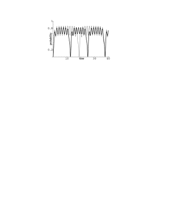
Figure 1a: Probability $P_{1}(t)$ at different values of $\varpi$.

Figure 1b: Detuning $\delta_{1}(t)$ at different values of $\varpi$.

Fig. 1b illustrates the time behavior of the detuning $\delta_{1}(t)$ calculated according to (21) for $a=0.015$, $\varpi=1/4$ and $\varpi=1/6$ (solid and dotted lines respectively) together with its limiting value corresponding to $\varpi=10^{-3}$ and $a=10^{-6}$ (dashed line). It is clearly seen from Fig. 1a that the period of slow oscillations grows when $\varpi$ decreases and fast oscillations go around the limiting value $0.75$ with the amplitude increasing with $\varpi$ decreasing. Moreover, Fig. 1b says that oscillating behavior of $P_{1}(t)$ is transformed into monotonically growing one when for $\varpi=0$ the detuning becomes a monotone function of time (dotted line on Fig 1b). If it acquires some oscillating perturbations the probability starts to oscillate also.

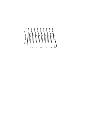
Figure 2a: Probability $P_{1}(t)$ at different values of $a$.

Figure 2b: Detuning $\delta_{1}(t)$ at different values of $a$.

The next two figures show the dependence of the same quantities on the parameter $a$ which is responsible for the phase shift in formula (29) at the fixed value $\varpi=1/5$. Dotted, dashed and solid lines (figure 2a) correspond to $a=0$, $a=0.02$ and $a=0.08$ respectively. Figure 2b shows the time dependence of the detuning $\delta(t)$ for $a=0$ (dotted line) and $a=0.08$ (solid line). From Fig. 2b we can conclude that the parameter $a$ defines mainly the maximum of the absolute value of the detuning which it takes at $t=0$. Fig. 2a says that the amplitude of fast oscillations grows together with $a$.

Figure 3: Probability $P_{1}(t)$ at different values of $\Omega_{0}$.

The next figure shows the dependence of $P_{1}(t)$ from the frequency of fast oscillations $\Omega_{0}$ at $a=0$ and $\varpi=0.2$. Dotted, solid and dashed lines correspond to $\Omega_{0}=2$, $\Omega_{0}=1.6$ and $\Omega_{0}=1.2$ respectively. More it differs from the critical value equal $2$ corresponding to $\xi^{2}=3f_{0}^{2}$, when the oscillations in formula (25) disappear, bigger the amplitude of the fast oscillations becomes.

6 Conclusion

Using the technique of intertwining operators for a Dirac-like system developed in [23] we have found time dependent electric fields for which the equation of motion for a two-level system placed in this field obtained after the rotating wave approximation can be solved exactly. Pseudosupersymmetry generators constructed with the help of intertwining operators together with the super-Hamiltonian close a quadratic deformation of the superalgebra constructed in [20]. We conclude, hence, that two-level systems in external electromagnetic fields may have hidden quadratic pseudosupersymmetry which is responsible for the new phenomenon consisting in disappearance of the Rabi oscillations.

References

References

-
[1]
Golfand Y A and Likhtman E P 1971 JETP Lett.
13 323;
Ramond P 1971 Phys. Rev. D3 2415;
Neveu A and Schwarz J 1971 Nucl. Phys. B31 86 - [2] Witten E 1981 Nucl. Phys. B188 513; 1982 Nucl. Phys. B202 253
- [3] Nakayama T. and DeWitt H 1964 J. Quant. Spectr. Radiative Transfer 4 623
- [4] Wong J 1967 J. Math. Phys. 8 2039
- [5] Baz’ A I, Zel’dovich Ya B and Perelomov A M 1969 Scattering, reactions and decay in non-relativistic quantum mechanics (Jerusalem: Israel Programm for Scientific Translations)
-
[6]
Baker H C 1984 Phys. Rev. A30 773
Ruschhaupt A, Delgado F and Muga J G 2005 J. Phys. A38 L171 - [7] Sparenberg J-M and Baye D 1996 Phys. Rev. C54 1309
- [8] Keldysh M V 1951 DAN USSR (Doklady Akademii Nauk SSSR) 77 11
- [9] Naimark M A 1969 Linear differential operators (Moscow: Nauka)
- [10] Marchenko V A 1977 Sturm-Liouvulle operators and their applications (Kiev: Naukova Dumka)
- [11] Bender C M and Boettcher S 1998 Phys. Rev. Lett. 24 5243
- [12] Bender C M, Brody D C and Jones H F, 2002 Phys. Rev. Lett. 89 270401 and 2004 92 119902 (erratum)
- [13] Bender C M, Brod J, Refig A and Reuter M 2004 J. Phys. A37 10139
- [14] Ramírez A and Mielnik B 2003 Rev. Mex. Fis 49 (S2) 130
- [15] Samsonov B F and Roy P 2005 J. Phys. A38 L249
- [16] Samsonov B F 2005 SUSY transformations between diagonalizable and non-diagonalizable Hamiltonians preprint quant/ph 0503075
-
[17]
Cannata F, Junker G and Trost J 1998
Phys. Lett. A246 219
Andrianov A, Cannata F, Dedonder J P and Ioffe M V 1999 Int. J. Mod. Phys. A14 2675
Bagchi B, Mallik S and Quesne C 2001 Int.J.Mod.Phys. A16 2859
Petrović J S, Milanović V and Ikonić Z 2002 Phys. Lett. A300 595
Fernández D J, Muños R and Ramos A 2003 Phys.Lett. A308 11
Rosas-Ortiz O and Muñoz R 2003 J. Phys A36 8497
Bagchi B, Bíla H, Jakubský V, Mallik S, Quesne C and Znojil M 2005 PT -symmetric supersymmetry in a solvable short-range model preprint quant-ph/0503035 -
[18]
Znojil M 2001 Czech. J. Phys. 51 420
Dorey P, Dunning C and Tateo R 2001 J. Phys. A 34 L391
Cannata F, Ioffe M V, Roychoudhury R and Roy P 2001 Phys.Lett. A281 305
Levai G and Znojil M 2002 J. Phys. A35 8793
Cannata F, Ioffe M V and Nishnianidze D N 2003 Phys.Lett. A310 344
Znojil M 2003 PT-symmetry and supersymmetry in “GROUP 24: Physical and Mathematical Aspects of Symmetries” (IOP Publishing, Bristol). pp. 629 - 632 (proceedings of the XXIV International Colloquium on Group Theoretical Methods in Physics, Paris, July 15-20, 2002, Institute of Physics Conference Series Nr. 173, Sect. 7, Ed. Jean-Pierre Gazeau, Richard Kerner, Jean-Pierre Antoine, Stephane Metens and Jean-Yves Thibon, preprint hep-th/0209062)
Bagchi B, Banerjee A, Caliceti E, Cannata F, Geyer H B Quesne C and Znojil M 2004 CPT -conserving Hamiltonians and their nonlinear supersymmetrization using differential charge-operators C Preprint hep-th/0412211 - [19] Znojil M, Cannata F, Bagchi B and Roychoudhury R 2000 Phys. Lett. B483 284
- [20] Mostafazadeh A 2002 J. Math. Phys. 43 205; 2002 Nuclear Physics B640 419
- [21] Klishevich S M and Plyushchay M S 2002 Nucl. Phys. B628 217
- [22] Orszag M 2000 Quantum optics (Berlin: Springer-Verlag)
- [23] Nieto L M, Pecheritsin A A and Samsonov B F 2003 Ann. Phys. (NY) 305/2 151
- [24] Bagrov V G and Samsonov B F 1995 Theor. Math. Phys. 104 1051
- [25] Bagrov V G, Baldiotti M C, Gitman D M and Shamshutdinova V V 2004 Darboux transformations of two-level systems preprint math-ph/0404078