Geometric Effects and Computation in Spin Networks

Abstract

When initially introduced, a Hamiltonian that realises perfect transfer of a quantum state was found to be analogous to an $x$-rotation of a large spin. In this paper we extend the analogy further to demonstrate geometric effects by performing rotations on the spin. Such effects can be used to determine properties of the chain, such as its length, in a robust manner. Alternatively, they can form the basis of a spin network quantum computer. We demonstrate a universal set of gates in such a system by both dynamical and geometrical means.

I Introduction

Many proposed schemes for quantum computation rely on nearest–neighbour couplings in order to generate a two qubit gate. However, during a computation, it is necessary to interact distant qubits. Typically, one would imagine a series of nearest neighbour SWAP operations to move two qubits together so that they can interact. Recently, the question of more efficient protocols has been addressed. In particular, a large set of different spin chains that permit perfect state transfer are now known Christandl et al. (2004); Albanese et al. (2004); Christandl et al. (2005); Karbach and Stolze (2005); Yung and Bose (2005); Shi et al. (2005). The first of these, defined for an $N$ qubit chain, was based on an analogy with a spin $J=\mbox{$\textstyle\frac{1}{2}$}(N-1)$ particle rotating about the $x$-axis from its $\left|\,M_{z}=J\right\rangle$ to $\left|\,M_{z}=-J\right\rangle$ state. In this paper we will show how to extend the analogy to achieve rotations about the $z$- and $y$-axes. We demonstrate a protocol that uses these in a geometric manner to determine properties of the chain, such as its length.

In parallel to the development of state transfer in single chains, Burgarth and Bose have concentrated on developing a protocol that allows perfect state transfer in pairs of chains with less stringent manufacturing requirements. Their initial demonstration Burgarth and Bose (2004) involved encoding the state to be transmitted across the inputs of two identical chains, but has culminated in a demonstration that the two chains need not be identical Burgath and Bose (2005). If we apply geometric or topological effects during transmission of a quantum state along a chain, then the action of the gate separates out from the visibility, i.e. the arrival probability of the state. Since the protocol of Burgarth and Bose guarantees perfect visibility, we can consider using this to realise a robust computation. We construct a universal set of spin networks that act on a quantum state as it is transmitted. These chains require no external interaction at all. However, the Hadamard gate is not geometric or topological in nature. We thus go on to develop a geometric Hadamard gate, by allowing adiabatic manipulation of particular inter-qubit couplings.

II Geometric Effects and Metrology of a Spin Chain

The perfect state transfer chain of Christandl et al. Christandl et al. (2004, 2005); Albanese et al. (2004) has a Hamiltonian of the form

$$H=\lambda\sum_{i=1}^{N-1}\frac{\sqrt{i(N-i)}}{4}(\sigma_{x}^{i}\sigma_{x}^{i+1}+\sigma_{y}^{i}\sigma_{y}^{i+1}).$$ (1)

This Hamiltonian has the property that it preserves total spin i.e. if, at time $t=0$, there is a single excitation in the system then, in the absence of external interactions, there will always be a single excitation present. In the first excitation subspace, using basis states $\left|\,n\right\rangle$ to denote the presence of the excitation on qubit $n$, the Hamiltonian is

$$\frac{\lambda}{2}\left(\begin{array}[]{ccccc}0&\sqrt{N-1}&0&...&0\\ \sqrt{N-1}&0&\sqrt{2(N-2)}&...&0\\ 0&\sqrt{2(N-2)}&0&...&0\\ 0&0&\sqrt{3(N-3)}&...&0\\ \vdots&\vdots&\vdots&\ddots&\sqrt{N-1}\\ 0&0&0&\sqrt{N-1}&0\\ \end{array}\right),$$

which is just the rotation matrix $J_{x}$ for a particle of spin $J=\mbox{$\textstyle\frac{1}{2}$}(N-1)$, scaled by a strength parameter $\lambda$. If the single excitation is on qubit $n$, then this is equivalent in the spin picture to being in the state $\left|\,M_{z}=J+1-n\right\rangle$. We can thus view state transfer between opposite ends of the chain as a rotation by an angle $\pi$ around the $x$-axis of the Bloch sphere. Similarly, we can use the Bloch sphere picture to understand that if we rotate by an angle of $\pi/2$, we will move from the state $\left|\,M_{z}=J\right\rangle$ to $\left|\,M_{y}=J\right\rangle$. However, with only the Hamiltonian $J_{x}$, the rotations that we can generate are limited. We will thus introduce a magnetic field gradient over the spin chain. This is equivalent to a rotation around the $z$-axis of the spin-$J$ particle, and takes the form

$$\frac{\kappa}{2}\left(\begin{array}[]{ccccc}N-1&0&0&...&0\\ 0&N-3&0&...&0\\ 0&0&N-5&...&0\\ \vdots&\vdots&\vdots&\ddots&0\\ 0&0&0&0&1-N\\ \end{array}\right)$$

in the first excitation subspace, where $\kappa$ is a coupling strength that we control. The implementation of such a gradient depends on the details of the physical system that we use to implement our spins. If we consider systems such as quantum dots Nikopoulos et al. (2004) that are equally spaced, then this field is just a linear gradient, which can be implemented comparitively easily and without local control of the system.

The situation that we envisage is that we have a chain with a fixed Hamiltonian, eqn. (1), of known $\lambda$ and that we can apply a gradient magnetic field. This is sufficient to be able to implement a geometric rotation with the following protocol.

1. Initialise the spin chain such that every spin is in the $\left|\,0\right\rangle$ state.

2. Place a single excitation at one end of the chain i.e. $\left|\,M_{z}=J\right\rangle$.

3. Wait for a time $\pi/(2\lambda)$, resulting in $\left|\,M_{y}=J\right\rangle$.

4. Switch on the magnetic gradient field at strength $\kappa$ for a time $\pi/\sqrt{\lambda^{2}+\kappa^{2}}$, which rotates the state to $\left|\,M_{y}=-J\right\rangle$.

5. Switch off the magnetic field, and wait for a time $\pi/(2\lambda)$.

This protocol returns the single excitation to its starting point, having followed great circles of the Bloch sphere, as depicted in Fig. 1. This means that no dynamic phase is generated. However, a solid angle

$$\Omega=2\tan^{-1}\left(\frac{\lambda}{\kappa}\right)$$

has been carved out, and the geometric phase of the state is thus Ekert et al. (2000); Shapere and Wilczek (1989)

$$\gamma=\mbox{$\textstyle\frac{1}{2}$}(N-1)\Omega.$$

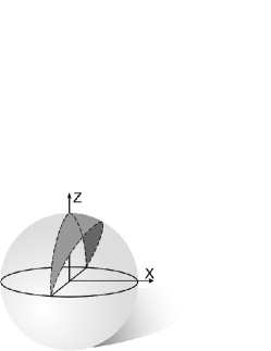
Figure 1: By performing rotations around great circles, there are no dynamical phases, making the result robust against some types of error.

Consider the case where a third party has manufactured a spin chain for us, and assures us that the state transfer time, $t_{0}=\pi/\lambda$, has a particular value. However, we do not know what the length of the chain is. In this case, we can perform interference experiments to determine the phase, and therefore the number of spins on the chain. In the absence of errors, a modified version of the semi-classical Fourier transform Griffiths and Niu (1996), combined with phase estimation, makes a particularly efficient determination. To achieve this, we start without a magnetic field, so that the state returns to the start of the chain with a phase of $\pi(N-1)$ i.e. a phase factor of $\pm 1$, determined by the parity of the chain length. With the initial state $(\left|\,0\right\rangle+\left|\,1\right\rangle)/\sqrt{2}$ on the first qubit, this evolves to the state $(\left|\,0\right\rangle-(-1)^{N}\left|\,1\right\rangle)/\sqrt{2}$. After performing another Hadamard on this qubit, it is in the state $\left|\,0\right\rangle$ or $\left|\,1\right\rangle$ depending on the parity of $N$. If we repeat this experiment, generating half the phase (using the aforementioned protocol, Fig. 1), then the possible phase-factors are $i$, $-1$, $-i$ and $1$. However, we know from the previous result that we will either get one of the pair $i$ or $-i$ or one of the pair $-1$ or $1$. If we know we’re going to get the $i$ phases, then we compensate for this with a $\sqrt{\sigma_{z}}$ gate before performing the Hadamard. Measurement of the first spin then gives the second least significant bit of the length of the chain. These steps can be repeated (halving the solid angle, $\Omega$, each time) to determine the next-least significant bit of $N$.

In the presence of errors, such as manufacturing errors or timing errors, or in the presence of noise (interaction of the chain with the environment), the semi-classical method fails because the measurement results become probabilistic. Instead, there are two ways that we can perform the experiment. Firstly, we might use the more standard interferometric geometrical phase technique Wagh and Rakhecha (1995), where we use the same magnetic field strength on every experiment, and apply a different $z$-rotation, $e^{i\sigma_{z}\chi}$, before applying the final Hadamard. The results that we plot, with varying $\chi$, are well described by the function

$$\mbox{$\textstyle\frac{1}{2}$}(1+\nu\cos(J\Omega-\chi))$$

and the offset of the maximum, $\chi_{0}=J\Omega$, determines the geometric phase, and thus the length of the chain. The quantity $\nu$ is known as the visibility and encapsulates some information about the errors that have occurred. However, it turns out that it is better to set $\chi=0$ and plot the arrival probability with varying $\Omega$ (i.e. the magnetic field strength). In this case, we just estimate the frequency of the curve, and that tells us the length of the chain. This method is superior because, not only is it stable against timing errors (Fig. 2(a)), but also against errors in the coupling strengths (Fig. 2(b)), which have no analogue in the spin picture.

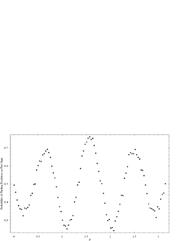
(a) Independent timing errors of up to $50\%$ for each of the 3 periods of evolution, averaged across 1000 runs.

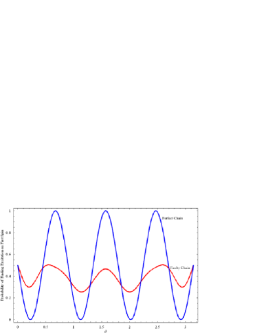
(b) Coupling errors of up to $80\%$ for each nearest-neighbour coupling in comparison to the ideal case. These errors are fixed for all experiments.

Figure 2: The effect of errors of arrival probability of the state, as a function of magnetic field strength $\kappa=\cot(\theta)$ for a chain of 8 spins.

When performing these experiments, we need to be aware that there may be an offset to the magnetic field gradient i.e. the gradient is the correct strength but the 0 of the field is not located on the centre of the chain. This manifests itself as an additional, dynamic, phase on the state. We can determine this shift using a simple modification of the previous protocol. Once in the $\left|\,M_{y}=J\right\rangle$ state, we turn on a magnetic gradient field of strength $\kappa$ and wait for a time $t=2\pi/\sqrt{\lambda^{2}+\kappa^{2}}$. Finally, we switch off the magnetic field and wait for a time $3\pi/2\lambda$ so that our state returns to its starting point. The geometric phase in this case is $2\pi(N-1)$, thus leaving us simply with the dynamical phase due to the offset of the magnetic field, which can be determined by a series of interference experiments. Alternatively, this modified protocol can be incorporated into the original one to remove the effect of the offset directly.

III Spin Networks Based on Perfect Transfer

So far, we have described how a spin chain with fixed couplings and a controllable magnetic field gradient can yield a geometric phase on a state. We will now demonstrate a powerful technique for modifying any of the spin chains found in the literature Albanese et al. (2004); Karbach and Stolze (2005); Yung and Bose (2005); Shi et al. (2005) to give networks (i.e. no longer simple chains) that perform non-trivial operations as a quantum state is transmitted along them. The intuition behind how these modifications work stems from understanding the projection method described in Christandl et al. (2005), which demonstrates that a hypercube, with spins associated with its vertices, is equivalent to the perfect state transfer chain. When such a projection is performed, there is a lot of freedom to choose how the spins of the hypercube can be grouped, and it is this freedom that we take advantage of.

(a) Spin chain that treats the state $(\left|\,01\right\rangle+\left|\,10\right\rangle)/\sqrt{2}$ like a single excitation on the original perfect state transfer chain.

(b) A perfect state transfer ring that could have an electric charge or magnetic field threaded through it, yielding a geometric or topological phase during transmission of a state between A and B.

Figure 3: Novel modifications of spin chains that result in state transfer. $J_{n}$ represents an exchange coupling between the indicated qubits, of strength $J_{n}=\lambda\sqrt{n(N-n)}/4$.

The two prime examples, from which all our modifications stem, are shown in Figs. 3(a) and 3(b). Consider the behaviour of the chain shown in Fig. 3(a). Let us apply the Hamiltonian of the chain to a state $(\left|\,01\right\rangle+\left|\,10\right\rangle)/\sqrt{2}$, defined across the left-most qubits. Both of these jump to the next spin, $\left|\,2\right\rangle$, with a strength $J_{1}/\sqrt{2}$. So, we define

$$\left|\,\tilde{1}\right\rangle=(\left|\,01\right\rangle+\left|\,10\right\rangle)/\sqrt{2},$$

and find that $H\left|\,\tilde{1}\right\rangle=J_{1}\left|\,2\right\rangle$, just as it does with the original, unmodified, spin chain. If we now consider the action of

$$H\left|\,2\right\rangle=\frac{J_{1}}{\sqrt{2}}(\left|\,01\right\rangle+\left|\,10\right\rangle)+J_{2}\left|\,3\right\rangle=J_{1}\left|\,\tilde{1}\right\rangle+J_{2}\left|\,3\right\rangle,$$

we see, again, that it acts in exactly the same was as the original chain, where the state $(\left|\,01\right\rangle+\left|\,10\right\rangle)/\sqrt{2}$ is treated as a single excitation. We can also verify that $(\left|\,01\right\rangle-\left|\,10\right\rangle)/\sqrt{2}$ is an eigenstate of the Hamiltonian, with eigenvalue 0. This means that such a state remains localised on those spins. Note that if we start with a quantum state on the right-most spin, then in the perfect state transfer time, this network acts as the optimal phase covariant cloner Chiara et al. (2004). The ring of Fig. 3(b) also behaves like a state transfer chain, where the excitations are $(\left|\,01\right\rangle+\left|\,10\right\rangle)/\sqrt{2}$ across the vertical pairs of qubits. Note, however, that these projection methods only work for the first excitation subspace. In the second excitation subspace there are significant differences - a single chain has a fermionic character, whereas the ring can allow two excitations in the pair of qubits.

IV Quantum Computation by Transmission Through Spin Networks

We have just seen that it is possible to split the original state transfer chain into networks that still allow perfect state transfer. Such modifications allow non-trivial unitary operations to be applied to a state as it is transferred. Since the spin chains are total spin preserving, the only operations that can be applied to a single spin are phase gates, which are not sufficient for universal quantum computation. Instead, we shall introduce the dual-rail encoding

$$\left|\,0_{L}\right\rangle = \left|\,01\right\rangle$$

$$\left|\,1_{L}\right\rangle = \left|\,10\right\rangle,$$

defined across the first qubit in each of two spin chains, which run in parallel. When the state is transmitted, we will extract the evolved state from the last qubit of each chain. Since these logical states both contain a single excitation, any single–qubit state contains a single excitation, and thus spin-preserving Hamiltonians are able to perform one–qubit rotations.

This encoding is exactly that considered in Burgarth and Bose (2004); Burgath and Bose (2005) for conclusive state transfer. In fact, any of the chains that we construct will behave like two independent chains operating in parallel, just with a basis change as the state moves along the chain. As such, we can still use the techniques of Burgarth and Bose to guarantee perfect visibility of the state, even in the presence of manufacturing errors. All we have to do is perform some initial experiments on the chains. Instead of plotting the arrival probability with time for the two independent chains, and finding times when the probabilities are equal, we plot the arrival probability of a single spin across the two output qubits. The two ‘chains’ that we have to compare simply correspond to having transmitted either the $\left|\,0_{L}\right\rangle$ or $\left|\,1_{L}\right\rangle$ states through the network. Such testing before using the networks as part of a computation also allows us to verify that the unitary operation is of sufficiently high fidelity.

A universal set of gates for quantum computation can be created out of an arbitrary $z$-rotation, a Hadamard and a two–qubit entangling gate. It is worth noting that phase gates can be applied to the dual-rail qubit by applying a phase gate to just one of the chains, and other types of rotation can be effected by making swaps between the two chains.

IV.1 Phase Gates

Structures such as the ring of Fig. 3(b) provide a suitable topology for examining the Aharanov-Bohm Aharonov and Bohm (1959) or Aharanov-Casher effects Aharanov and Casher (1984). The precise effect that we take advantage of depends on the particular physical implementation of our spins. As a concrete example, consider each spin being an empty quantum dot, and we introduce a single electron to act as the excitation. This situation has recently been discussed in the context of state storage Giampaolo et al. (2005). In this realisation, the magnetic gradient that we had previously is created with an electric field gradient. By threading a magnetic field through the centre of the ring, we realise the Aharanov-Bohm effect, which results in a phase of $\phi$ if the electron moves around the ring. If there are $L$ links around the loop, then we can assume that the electron gains a phase of $\delta=\phi/L$ as it jumps forwards, and $-\delta$ as it jumps back again. Hence, in the first excitation subspace, the Hamiltonian can be written as

$$H=\cos(\delta)J_{x}+\sin(\delta)J_{y}.$$

This just rotates the vector of our Hamiltonian by an angle $\delta$ about the $z$-axis. Hence, we still get perfect state transfer in the time $\pi/\lambda$. As noted in Christandl et al. (2005), the state gains an additional phase $\phi$ during transmission. This phase is topological in nature, and thus makes a robust $z$-rotation of a state during its transmission.

These rings are not limited to charged systems; we might alternatively use rings of magnetically sensitive spins and take advantage of the dual, Aharanov-Casher, effect Balatsky and Altshuler (1993).

IV.2 Hadamard Gate

(a) Hadamard gate.

(b) Arbitrary single qubit rotation, through specification of the parameters $\beta$, $\gamma$ and $\delta$.

Figure 4: Two spin chain networks that are equivalent to perfect state transfer chains, but perform non–trivial operations on encoded qubits, $\left|\,01\right\rangle$ and $\left|\,10\right\rangle$, as they are transmitted from left to right.

A Hadamard rotation is sufficient to convert $z$-rotations into any arbitrary single–qubit gate. The creation of such a gate follows from Fig. 3(a), where a state of $(\left|\,01\right\rangle+\left|\,10\right\rangle)/\sqrt{2}$ is transferred as a single excitation to the opposite end of a chain. Similarly, if we were to use an altered form, where one of the $J_{1}/\sqrt{2}$ couplings is replaced by $-J_{1}/\sqrt{2}$, then it would be the state $(\left|\,01\right\rangle-\left|\,10\right\rangle)/\sqrt{2}$ that gets transferred. Taking the outputs of these two networks as the logical qubit, then we see that a Hadamard rotation has been performed.

$$\frac{1}{\sqrt{2}}(\left|\,0_{L}\right\rangle+\left|\,1_{L}\right\rangle) \rightarrow \left|\,0_{L}\right\rangle$$

$$\frac{1}{\sqrt{2}}(\left|\,0_{L}\right\rangle-\left|\,1_{L}\right\rangle) \rightarrow \left|\,1_{L}\right\rangle$$

This leads us to test the Hadamard gate as shown in Fig. 4(a), which is created by running these two structures in parallel. We find that this acts as a unit which is capable of replacing any section of parallel chains (acting with a strength $\sqrt{2}$) and, as such, can be integrated to give circuits like that of Fig. 4(b) - an arbitrary one–qubit gate, where the phases of $\beta$, $\gamma$ and $\delta$ result from looping around magnetic fields (not shown) along the relevant sections.

IV.3 Two–Qubit Gates

We have demonstrated the ability to create an arbitrary single–qubit rotation, acting on a dual rail qubit, by using two parallel spin chains and interlinking them. We need no control after initial manufacture if we assume perfect circuits. We would therefore like to address the question of whether or not we can create a complete circuit of spins for performing a quantum algorithm, without the requirement of having to interact with the circuit. To do this, we need to show how to integrate a two–qubit gate, which would complete a universal set of gates.

One of our single qubit gates, the Hadamard, took the form of a unit that could, by suitable scaling of the couplings, be used to replace any sections of chain that run in parallel. We would like to find a two–qubit gate that behaves in a similar way. So, assuming that we have two qubits (i.e. four chains), is it possible to create an entangling operation between them? The problem with connecting four chains where the two pairs of chains have a single excitation each is that we are no longer in the first excitation subspace and perfect state transfer is not guaranteed in the second excitation subspace.

Without a two–qubit gate that can be integrated into our networks, we need to demonstrate some other form of two–qubit gate, and show how to move states between it and the one–qubit gate networks. In fact, the original state transfer chain has been shown to apply controlled-phase gates between all states stored on the chain Yung and Bose (2005); Clark et al. (2004). This is because the chain inverts the order of states during transmission. Since these states behave like fermions, they gain a topological phase factor of -1 on exchange. This can be used to create a suitable interaction between our logical qubits, by placing one of the qubits from each pair on the chain, and allowing state transfer to take place. This generalises to creating multi-qubit entangled states by placing one half of each logical qubit onto the chain.

IV.4 Joining Spin Chains

With this form of two–qubit gate, we need to be able to join it with other sections of chain, while minimising our interaction with them. In particular, we are currently required to quickly swap states between chains as they arrive (where ‘quick’ is in comparison to the transfer time $\pi/\lambda$). Previous works on state transfer have implicitly assumed this for the purpose of moving the state on and off the chain.

To do this, we introduce the idea of a switch, where we act on specific qubits, decoupling them from neighbouring qubits. There are two ways in which this can be implemented. Firstly, we can introduce a large, local, detuning (i.e. a magnetic field) Benjamin and Bose (2003). However, this requires a finely tuned, controllable, local field, which is technically difficult.

Instead, we consider the case where a spin has not only its computational states, $\left|\,0\right\rangle$ and $\left|\,1\right\rangle$, but also an auxiliary state, $\left|\,2\right\rangle$. By performing the transition $\left|\,0\right\rangle\rightarrow\left|\,2\right\rangle$, this blocks the $\sigma_{x}\sigma_{x}+\sigma_{y}\sigma_{y}$ coupling from causing the excitation to jump to this spin. As demonstrated in Fig. 5, two different types os switch are sufficient. The switches $\otimes$ and $\oplus$ have different auxiliary states, $\left|\,2\right\rangle$ and, as such, they can be addressed by different, global, fields e.g. by different lasers. If the levels, $\left|\,2\right\rangle$, are at the same energy as the computational states, then the accuracy of this clocking method is only limited by the speed at which the $\left|\,0\right\rangle\rightarrow\left|\,2\right\rangle$ transition can be performed in comparison to the state transfer time. For an external field of strength $\gamma$, the fidelity, $f\approx 1-\alpha/\gamma^{2}$, since this acts like a timing error on the state transfer process Christandl et al. (2005). If the auxiliary levels are at energies $E_{\otimes}$ and $E_{\oplus}$ above the levels of the computational states, then spontaneous emission adds to the inaccuracy of the scheme. This can be reduced by keeping the switching fields active while the switches should be in the $\left|\,2\right\rangle$ state Benjamin et al. (2004).

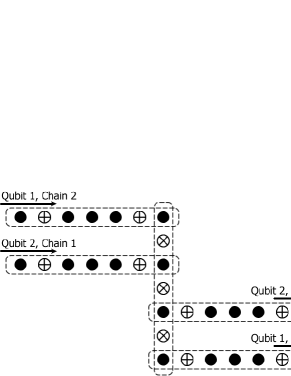
Figure 5: The qubits $\otimes$ and $\oplus$ act as two different types of switch. If they have an extra state, $\left|\,2\right\rangle$, which can be populated by a global pulse, such as a laser, then when both switch types are in this state, the state which we are computing is trapped. Moving the one type of switch back to the $\left|\,0\right\rangle$ state allows the computation to proceed in a fixed direction. The dashed boxes indicated engineered spin chains which perform state transfer.

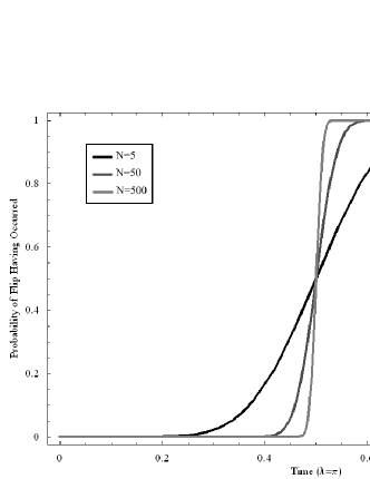
Figure 6: As the length of the spin chain increases, we can achieve an increasing sharp flip of the target spin at regular intervals.

The required control over the two global fields can be reduced by noting that the transition can be performed at fixed intervals of $2\pi/\lambda$ if we create all our spin chains so that they have the same state transfer time. In this situation, we can consider internalising the switch (i.e. removing the global fields) by using more spin chains. This is achieved by creating a form of controlled-NOT gate, resulting from consideration of the Hamiltonian

$$H=\sum_{i=1}^{N-1}K_{i}(\sigma_{x}^{i}\sigma_{x}^{i+1}+\sigma_{y}^{i}\sigma_{y}^{i+1})+\eta(\sigma_{z}^{N}\otimes\sigma_{x}^{N+1}-\sigma_{x}^{N+1}).$$

When we write out the Hamiltonian in a direct sum form, there is a $2N\times 2N$ subspace that governs the evolution of the basis states $\left|\,n,0\right\rangle$ and $\left|\,n,1\right\rangle$, where the $n$ represents the location of a single excitation on the first $N$ qubits of the chain, and the second component represents the state of the final, target, qubit. This matrix is identical to the Hamiltonian of a symmetric chain of length $2N$. We can therefore equate these coefficients with those of a $2N$-spin perfect transfer chain, $K_{i}=\sqrt{i(2N-i)}/4$ and $\eta=N/4$ such that in a time $2\pi/\lambda$, we find that

$$\left|\,1,0\right\rangle\rightarrow\left|\,1,1\right\rangle.$$

The $\left|\,0,0\right\rangle$ state remains unchanged, so this is a controlled-NOT gate. The probability that the target qubit is in the $\left|\,1\right\rangle$ state is

$$p=\sum_{n=N+1}^{2N}\sin^{2n-2}\left(\frac{\lambda t}{2}\right)\cos^{4N-2n}\left(\frac{\lambda t}{2}\right)\binom{2N-1}{n-1}.$$

Plotting this function (or writing as a hypergeometric function) makes it clear that the result is an increasingly sharp flip of the target qubit at times $(r+\mbox{$\textstyle\frac{1}{2}$})\pi/\lambda$ (integer $r$) as the length of the control chain increases (Fig. 6). Note, however, that the target of this operation is not a chain, but a single qubit.

If we were able to implement this type of interaction (it has an unphysical $\sigma_{z}\otimes\sigma_{x}$ term), we could choose to implement the switch, where the $\sigma_{x}$ targets the switch qubit on another chain, and acts between the $\left|\,0\right\rangle$ and $\left|\,2\right\rangle$ states. This results in a flip to the $\left|\,2\right\rangle$ state, which is assumed to be stable. If we do not have a stable $\left|\,2\right\rangle$ state, then the controlled-NOT can be used to target an auxiliary qubit, which is connected as depicted in Fig. 7. This introduces a local detuning which is periodically switched on and off, blocking the state transfer as required Benjamin and Bose (2003).

Figure 7: The target of a controlled-NOT gate can conditionally activate large Zeeman terms in the spin chain which cause reflection rather than transmission. A single large Zeeman term, $\gamma$, blocks transmission of states through the chain depending on the lower, auxiliary qubit.

V Non-Abelian Geometric Gates

We have demonstrated how, in principle, we can create an entire network of spins to perform a particular computation. However, we have also seen that by introducing a limited form of control (a magnetic field gradient), phase gates can be made geometric in nature, yielding a robustness against a variety of errors. We will now show how to create a Hadamard gate with geometric stability, for which we invoke a non-abelian geometric phase.

Figure 8: Two coupled perfect state transfer chains. Adiabatic varying of the parameters $\theta$ and $\phi$ gives a non-abelian geometric phase. The logical states of the qubit are defined by two degenerate eigenvectors.

To realise a non-abelian geometric phase, we require spin networks with degenerate eigenvalues. Consider, therefore, two perfect state transfer chains, both of length $N$, where we retain the dual-rail encoding. There are degenerate eigenvalues because everything is repeated in comparison to a single chain. We can make some small modification to these chains, linking them as shown in Fig. 8. This allows the introduction of two free parameters, $\theta$ and $\phi$, that control the coupling. The eigenvectors of maximum eigenvalue for this system are

$$\left|\,\psi_{1}\right\rangle = \frac{1}{\sqrt{2^{N-1}}}\left(\sum_{n=1}^{R}\sqrt{\binom{N-1}{n-1}}\left|\,n\right\rangle+\sum_{n=R+1}^{N}\sqrt{\binom{N-1}{n-1}}\left[\cos\left(\frac{\theta}{2}\right)\left|\,n\right\rangle-\sin\left(\frac{\theta}{2}\right)e^{-i\phi}\left|\,n^{\prime}\right\rangle\right]\right)$$

$$\left|\,\psi_{2}\right\rangle = \frac{e^{-i\phi}}{\sqrt{2^{N-1}}}\left(\sum_{n=1}^{R}\sqrt{\binom{N-1}{n-1}}\left|\,n^{\prime}\right\rangle+\sum_{n=R+1}^{N}\sqrt{\binom{N-1}{n-1}}\left[\cos\left(\frac{\theta}{2}\right)\left|\,n^{\prime}\right\rangle+\sin\left(\frac{\theta}{2}\right)e^{i\phi}\left|\,n\right\rangle\right]\right),$$

as can be readily verified. We can place a dual-rail encoded qubit into these eigenstates by applying a magnetic gradient of strength $\lambda$ for a time $\pi/(\sqrt{2}\lambda)$.

We will now consider a path in the parameter space $(\theta,\phi)$ that goes from $(0,0)\rightarrow(\theta,0)\rightarrow(\theta,\phi)\rightarrow(0,\phi)$. If we start our state in a degenerate eigenspace, then it remains in this space when these parameters are varied adiabatically. By differentiating the states $\left|\,\psi_{1}\right\rangle$ and $\left|\,\psi_{2}\right\rangle$ with respect to $\theta$ and $\phi$ Vedral (2003), we find that

$$\frac{\partial}{\partial\zeta}\left(\begin{array}[]{c}a_{1}\\ a_{2}\end{array}\right)=A_{\zeta}\left(\begin{array}[]{c}a_{1}\\ a_{2}\end{array}\right)$$

for $\zeta\in\{\theta,\phi\}$, where $a_{i}$ are the amplitudes of our state in the two different eigenvectors. The matrices, $A_{\zeta}$, are given by

$$A_{\theta} = i\frac{P}{2}\sigma_{y}$$

$$A_{\phi} = \frac{i}{2}(P\sin\theta\sigma_{x}+(1-P+P\cos\theta)\sigma_{z})$$

(up to an identity matrix, which only contributes a global phase) where

$$P=\frac{2}{2^{N}}\sum_{n=R+1}^{N}\binom{N-1}{n-1}.$$

Since both $A_{\zeta}$ are independent of $\zeta$, evaluating the evolution just involves exponentiating the matrices. For convenience, we define the variable $s$ such that $A_{\phi}^{2}=-s^{2}\leavevmode\hbox{\small 1\kern-3.8pt\normalsize 1}.$ We can therefore evaluate the whole evolution as we vary the parameters

$$U = e^{-i\frac{P\theta}{2}\sigma_{y}}e^{A_{\phi}\phi}e^{i\frac{P\theta}{2}\sigma_{y}}$$

$$= \leavevmode\hbox{\small 1\kern-3.8pt\normalsize 1}\cos\left(s\phi\right)+\frac{i}{s}e^{-iP\theta\sigma_{y}}\sin\left(s\phi\right)A_{\phi}.$$

The Hadamard gate is defined as $H=(X+Z)/\sqrt{2}$, so we select $\phi=\frac{\pi}{2s},$ resulting in the evolution

$$U=\frac{i}{s}\left((P\sin((P+1)\theta)+\sin(P\theta)(1-P))\sigma_{x}+(\cos(P\theta)(1-P)+P\cos((P+1)\theta))\sigma_{z}\right).$$

For a given value of $P$, we just have to solve for $\theta$. In particular, for $R=N/2\Rightarrow P=\mbox{$\textstyle\frac{1}{2}$}$, we find that $\theta=\pi/4$ and $\phi=\pi/\cos(\pi/8)$. Similarly, if $R=1$, and assuming a long chain, we find that $\theta\approx\pi/8$ and $\phi\approx\pi$.

Finally, we should rotate back from the eigenstates of the chain to being on the first (or last) spins of the chains by applying the gradient magnetic field.

VI Conclusions

In this paper, we have demonstrated a number of widely applicable techniques for modifying spin chains so that they can perform non-trivial operations on encoded states. We have created a universal set of both dynamic and geometric gates on these spin chains. The geometric gates are particularly interesting because these gates effectively make the statement “if the state has arrived, they have undergone the desired evolution”. When coupled with the conclusive state transfer protocol of Burgarth and Bose, Burgath and Bose (2005), this guarantees arrival of a correctly evolved state, even in imperfect spin networks.

The geometric gates, while being much more robust, require a greater degree of control over the system. The ‘dynamic’ gates that we have demonstrated require no external interaction after initial manufacture (assuming they have a tolerable fidelity, which can be tested), which result in the idea of fixed circuits of quantum spins. Since they need no interaction (except for the input of initial states, and the measurement of final states), we can, in principle, completely isolate the system from the environment and practically eliminate decoherence.

In addition, the techniques described here may be usefully reinterpreted in many different contexts. For example, the non-abelian geometric phase gate that we have demonstrated can be translated into atomic systems, in a fundamentally different way to the more standard ‘tripod’ system Unanyan et al. (1999); Duan et al. (2001) that has been extensively studied. It is, instead, like the less-studied system introduced by Karle and Pachos Karle and Pachos (2003). Alternatively, the state transfer techniques may be of interest in control theory. Here, the question of coherent population transfer between the levels of an $N$-level atom is considered. Cook and Shore Cook and Shore (1979) originally demonstrated how a state can be transferred from one level to another, using a single pulse, with a scheme that is exactly equivalent to the original state transfer chain. Coupling schemes such as that of Fig. 3(a), and its generalisation, would allow modification of that idea to transfer a known superposition of two, or more, levels to another level of the spin.

We thank Simon Benjamin, Artur Ekert and Daniel K.L. Oi for useful discussions. ME acknowledge financial support from Swedish Research council. AK is supported by UK EPSRC.

References

- Christandl et al. (2004) M. Christandl, N. Datta, A. Ekert, and A. J. Landahl, Phys. Rev. Lett. 92, 187902 (2004).
- Albanese et al. (2004) C. Albanese, M. Christandl, N. Datta, and A. Ekert, Phys. Rev. Lett 93, 230502 (2004).
- Christandl et al. (2005) M. Christandl, N. Datta, T. Dorlas, A. Ekert, A. Kay, and A. Landahl, Phys. Rev. A 71, 032312 (2005).
- Karbach and Stolze (2005) P. Karbach and J. Stolze (2005), quant-ph/0501007.
- Yung and Bose (2005) M.-H. Yung and S. Bose, Phys. Rev. A 71, 032310 (2005).
- Shi et al. (2005) T. Shi, Y. Li, Z. Song, and C. P. Sun, Phys. Rev. A 71, 032309 (2005).
- Burgarth and Bose (2004) D. Burgarth and S. Bose (2004), quant-ph/0406112.
- Burgath and Bose (2005) D. Burgath and S. Bose (2005), quant-ph/0502186.
- Nikopoulos et al. (2004) G. Nikopoulos, D. Petrosyan, and P. Lambropoulos, J. Phys.:Condens. Matter 16, 4991 (2004).
- Ekert et al. (2000) A. Ekert, M. Ericsson, P. Hayden, H. Inamori, J. A. Jones, D. K. L. Oi, and V. Vedral, J. Mod. Opt 47, 2501 (2000).
- Shapere and Wilczek (1989) A. Shapere and F. Wilczek, eds., Geometric Phases in Physics, vol. 5 of Advanced Series in Mathematical Physics (World Scientific, Singapore, 1989).
- Griffiths and Niu (1996) R. B. Griffiths and C. Niu, Phys. Rev. Lett. 76, 3228 (1996).
- Wagh and Rakhecha (1995) A. G. Wagh and V. C. Rakhecha, Phys. Lett. A 197, 107 (1995).
- Chiara et al. (2004) G. D. Chiara, R. Fazio, C. Macchiavello, S. Montanegro, and G. M. Palma, Phys. Rev. A 70, 062308 (2004).
- Aharonov and Bohm (1959) Y. Aharonov and D. Bohm, Phys. Rev. 115, 485 (1959).
- Aharanov and Casher (1984) Y. Aharanov and A. Casher, Phys. Rev. Lett. 53, 319 (1984).
- Giampaolo et al. (2005) S. M. Giampaolo, F. Illuminati, A. D. Lisi, and S. D. Siena (2005), quant-ph/0503107.
- Balatsky and Altshuler (1993) A. V. Balatsky and B. L. Altshuler, Phys. Rev. Lett. 70, 1678 (1993).
- Clark et al. (2004) S. Clark, C. Moura-Alves, and D. Jaksch (2004), quant-ph/0406150.
- Benjamin and Bose (2003) S. C. Benjamin and S. Bose, Phys. Rev. Lett. 90, 247901 (2003).
- Benjamin et al. (2004) S. C. Benjamin, B. W. Lovett, and J. H. Reina, Phys. Rev. A 70, 060305 (2004).
- Vedral (2003) V. Vedral, Int. J. Quantum Inf. 1, 1 (2003).
- Unanyan et al. (1999) R. G. Unanyan, B. W. Shore, and K. Bergmann, Phys. Rev. A 59, 2910 (1999).
- Duan et al. (2001) L.-M. Duan, J. I. Cirac, and P. Zoller, Science 292, 1695 (2001).
- Karle and Pachos (2003) R. Karle and J. Pachos, J. Math. Phys 44, 2463 (2003).
- Cook and Shore (1979) R. J. Cook and B. W. Shore, Phys. Rev. A 20, 539 (1979).