Rabi spectroscopy for a two-level system

Abstract

We have analyzed the interaction of a dissipative two level quantum system with high and low frequency excitation. The system is continuously and simultaneously irradiated by these two waves. If the frequency of the first signal is close to the level separation and the second one is tuned to the Rabi frequency, it is shown that the response of the system exhibits an undamped low frequency oscillation. The method can be useful for low frequency Rabi spectroscopy in various physical systems which are described by a two level Hamiltonian, such as nuclei spins in NMR, double well quantum dots, superconducting flux and charge qubits, etc. As an example, the application of the method to the readout of a flux qubit is considered.

It is well known that under resonant irradiation, a quantum two level system (TLS) can undergo coherent (Rabi) oscillations. Such oscillations occur if microwaves are in resonance with the spacing between the energy levels. In this case the level occupation probability will oscillate with a frequency proportional to the amplitude of resonant field Rabi . The effect is widely used in molecular beam spectroscopy  beam , and in quantum optics Raimond .

Normally, such oscillations are damped out with a rate, which is dependent on how strongly the system is coupled to the environment. In recent years, progress in the investigations of scalable solid state qubits has necessitated the development of different methods of advanced qubit control. One of the proposals in this direction was to maintain the Rabi oscillations for arbitrary long times by the synchronization of the phase of Rabi oscillations, with that of the ideal solid state detector with the aid of a quantum feedback loop  Korotkov3 .

In this work we propose another method for maintaining such oscillations. We consider a TLS which is irradiated continuously by two external sources. The first one with a frequency $\omega_{0}$, which is close to the energy gap between the two levels, excites the low frequency Rabi oscillations. A second, low frequency source tuned to the Rabi frequency causes the oscillations to persist.

We start with a Hamiltonian of a TLS subjected to a both high and low frequency excitation:

$$H=\frac{\Delta}{2}\sigma_{x}+\frac{\varepsilon}{2}\sigma_{z}-\sigma_{z}F\cos\omega_{0}t-\sigma_{z}G(t).$$ (1)

Hamiltonian  (1) is written in the localized state basis. Here $\Delta$ is the tunnelling rate between localized states, $\varepsilon$ is the bias, F is the coupling between the TLS and high frequency field, and G(t) is a low frequency external force. In the eigenstates basis, which we denote by upper case subscripts for the Pauli matrices $\sigma_{X},\sigma_{Y},\sigma_{Z}$, Hamiltonian  (1) reads:

$$H=\left[{\frac{\Delta}{\Delta_{\varepsilon}}F\cos\omega_{0}t+\frac{\Delta}{\Delta_{\varepsilon}}G(t)}\right]\sigma_{X}$$

$$+\left[{\frac{\Delta_{\varepsilon}}{2}-\frac{\varepsilon}{\Delta_{\varepsilon}}F\cos\omega_{0}t-\frac{\varepsilon}{\Delta_{\varepsilon}}G(t)}\right]\sigma_{Z},$$ (2)

where $\Delta_{\varepsilon}=\sqrt{\Delta^{2}+\varepsilon^{2}}$ is the gap between two energy states.

A more realistic description of the TLS requires the inclusion of the dissipative environment in Hamiltonian (1), which for a spin-boson model of the bath results in the Bloch-Redfield equations for the matrix operators $\sigma_{X}$, $\sigma_{Y}$, $\sigma_{Z}$, Bloch , Hartmann . For weak driving ($f\ll\Delta$), and for weak coupling of the TLS to the bath these equations can be approximated by Bloch-type equations Saito :

$$\left\langle{\dot{\sigma}_{Z}}\right\rangle=\left({2f\cos\omega_{0}t+2g(t)}\right)\left\langle{\sigma_{Y}}\right\rangle-\Gamma_{Z}\left(\left\langle{\sigma_{Z}}\right\rangle-Z_{0}\right),$$ (3)

$$\left\langle{\dot{\sigma}_{Y}}\right\rangle=-\left({2f\cos\omega_{0}t+2g(t)}\right)\left\langle{\sigma_{Z}}\right\rangle$$

$$+\left[{\frac{\Delta_{\varepsilon}}{\hbar}-\frac{{2\varepsilon}}{\Delta}f\cos\omega_{0}t-\frac{{2\varepsilon}}{\Delta}g(t)}\right]\left\langle{\sigma_{X}}\right\rangle-\Gamma\left\langle{\sigma_{Y}}\right\rangle,$$ (4)

$$\left\langle{\dot{\sigma}_{X}}\right\rangle=-\left[{\frac{\Delta_{\varepsilon}}{\hbar}-\frac{{2\varepsilon}}{\Delta}f\cos\omega_{0}t-\frac{{2\varepsilon}}{\Delta}g(t)}\right]\left\langle{\sigma_{Y}}\right\rangle-\Gamma\left\langle{\sigma_{X}}\right\rangle,$$ (5)

where $f=\Delta$F$/\hbar\Delta_{\varepsilon}$, $g(t)=\Delta$G(t)$/\hbar\Delta_{\varepsilon}$, and $Z_{0}=-\tanh\left(\Delta_{\varepsilon}/k_{B}T\right)$ is the equilibrium polarization of the system in the absence of external excitation sources ($f=0$, $g=0$). The angled brackets in Eqs. (3), (Rabi spectroscopy for a two-level system), and (5) denote the trace over reduced density matrix $\rho(t)$, which is obtained by tracing out all environment degrees of freedom: $\langle\sigma_{X}\rangle=Tr(\sigma_{X}\rho(t))$, etc. In order to simplify the problem we assume the relaxation, $\Gamma_{Z}$ and dephasing, $\Gamma$, rates in (3)-(5) are time-independent, i.e. the rates are slowly varying functions on the scale of Rabi period which is on the order of $1/f$.

The desired solution of Eqs. (3), (Rabi spectroscopy for a two-level system), and (5) is:

$$\left\langle{\sigma_{Z}}\right\rangle=Z(t),$$ (6)

$$\left\langle{\sigma_{Y}}\right\rangle=Y(t)+A(t)\cos(\omega_{0}t)+B(t)\sin(\omega_{0}t),$$ (7)

$$\left\langle{\sigma_{X}}\right\rangle=X(t)+C(t)\cos(\omega_{0}t)+D(t)\sin(\omega_{0}t),$$ (8)

where the quantities $X$, $Y$, $Z$, $A$, $B$, $C$, and $D$ are slowly varying, compared to the high frequency $\omega_{0}$ operators. In the rotating wave approximation we obtain from Eqs. (3), (Rabi spectroscopy for a two-level system), and (5) the response of the system to a small external force $g(t)$. The Fourier components for the slowly varying $A(\omega)$, and $B(\omega)$, and for the low frequency persistent response of the TLS to a small low frequency excitation, $Z(\omega)$, $Y(\omega)$, and $X(\omega)$ are as follows: $C(\omega)=B(\omega)$, $D(\omega)=-A(\omega)$,

$$Z(\omega)=g(\omega)\frac{{2\varepsilon}}{\Delta}f^{2}P_{Z}Z_{0}\frac{\delta}{{\delta^{2}+\Gamma^{2}}}\frac{{2\Gamma+i\omega}}{s(\omega)},$$ (9)

$$A(\omega)=g(\omega)\frac{{2\varepsilon}}{\Delta}f{\kern 1.0pt}P_{Z}Z_{0}\frac{\delta}{{\delta^{2}+\Gamma^{2}}}\frac{{\left({2\Gamma+i\omega}\right)\left({i\omega+\Gamma_{Z}}\right)}}{s(\omega)},$$ (10)

$$B(\omega)=-g(\omega)\frac{{2\varepsilon}}{\Delta}f{\kern 1.0pt}P_{Z}Z_{0}\frac{\delta}{{\delta^{2}+\Gamma^{2}}}\frac{1}{{\left({\delta^{2}+(\Gamma+i\omega)^{2}}\right)}}{\rm{}}\left\{{\frac{{f^{2}\delta\left({2\Gamma+i\omega}\right)}}{s(\omega)}-\frac{{\delta^{2}-\Gamma^{2}-i\omega\Gamma}}{\delta}}\right\},$$ (11)

$$Y(\omega)=\frac{\hbar}{\Delta_{\varepsilon}}\frac{\varepsilon}{\Delta}fA(\omega)+\left({\frac{\hbar}{\Delta_{\varepsilon}}}\right)^{2}\left({2g(\omega)P_{Z}Z_{0}-\frac{\varepsilon}{\Delta}fB(\omega)}\right)\left({\Gamma+i\omega}\right),$$ (12)

$$X(\omega)=\left({\frac{\hbar}{\Delta_{\varepsilon}}}\right)^{2}\frac{\varepsilon}{\Delta}fA(\omega)\left({\Gamma+i\omega}\right)-\frac{\hbar}{\Delta_{\varepsilon}}\left({2g(\omega)P_{Z}Z_{0}-\frac{\varepsilon}{\Delta}fB(\omega)}\right),$$ (13)

where $\delta$ is a high frequency detuning, $\delta=\omega_{0}-\Delta_{\varepsilon}/\hbar$, $\Omega_{R}$ is the Rabi frequency, $\Omega_{R}=\sqrt{\delta^{2}+f^{2}}$, $s(\omega)=(\Omega_{R}-\omega+i\Gamma)(\Omega_{R}+\omega-i\Gamma)(i\omega+\Gamma_{Z})-f^{2}\left({\Gamma_{Z}-\Gamma}\right)$, and

$$P_{Z}=\frac{{\Gamma_{Z}\left({\Gamma^{2}+\delta^{2}}\right)}}{{\Gamma_{Z}\left({\Gamma^{2}+\delta^{2}}\right)+f^{2}\Gamma}}.$$ (14)

$P_{Z}Z_{0}$ is the nonequilibrium polarization, i. e., the steady state population difference between the qubit energy levels in the case when the high frequency excitation is applied to the qubit. When deriving the expressions  (9)- (13) we assume the force $g$ to be small, thereby we neglect the higher order terms of $g$. In addition, we keep only the terms which oscillate within the bandwidth of the Rabi frequency and neglect the terms which are of the order of $\hbar f/\Delta_{\varepsilon}$, $\hbar\Gamma/\Delta_{\varepsilon}$, $\hbar\Gamma_{Z}/\Delta_{\varepsilon}$.

As is seen from these expressions the persistent low frequency oscillations of the spin components $Z(t)$, $X(t)$, $Y(t)$ appear as the response to the low frequency external force, $g(t)$, only in the presence of the high frequency excitation ($f\neq 0$).

Exactly at resonance ($\delta=0$) $A(\omega)=0$, $Z(\omega)=0$, but $B(\omega)\neq 0$. Hence, as is seen from Eqs. (6), (7), (8), in this case the population of the two levels are equalized, spin circularly rotates in the $XY$ plane with frequency $\omega_{0}$, with the center of the circle being precessed with the Rabi frequency.

The key point of the method we described above is that it allows for the detection of the high frequency response of a TLS at a frequency which is much less than the gap frequency. The low frequency dynamics of the quantities $\left\langle{\sigma_{X}}\right\rangle,\left\langle{\sigma_{Y}}\right\rangle$, $\left\langle{\sigma_{Z}}\right\rangle$ bears information about the relaxation, $\Gamma_{Z}$, and dephasing, $\Gamma$, rates. The experimental realization of this method requires the measurement of the difference of low frequency response of the system of interest with and without high frequency excitation.

The detection scheme depends on the problem under investigation. For example, the method can easily be adapted for NMR. As is seen from (1), the NMR case corresponds to the polarization of the sample with the fields $\triangle$ and $\varepsilon$ along the $x$ and $z$ axes, respectively, with a high frequency excitation $Fcos(\omega_{0}t)$ and a low frequency probe $G(t)$ being applied along the $z$ axis.

Another example are the macroscopic quantun TLS, such as superconducting qubits based on mesoscopic Josephson junctions Makhlin . For these qubits the Rabi oscillations have been detected through the statistics of switching events Nakamura ; Vion ; Martinis ; Chiorescu . In parallel, the detection of coherent oscillations through a weak continuous measurement which does not destroy the quantum coherence of the TLS was proposed Averin ; Korotkov1 ; Korotkov2 . Generally, the signature of such oscillations can be found in the noise spectrum of the TLS, which was recently demonstrated for a superconducting flux qubit Il'ichev . Let us consider last example in more detail, namely, the application of the method to a persistent current qubit, which is a superconducting loop interrupted by three Josephson junctions  Mooij , Orlando . The basis qubit states have an opposing persistent current and the operator of the persistent current in the qubit loop reads $\widehat{I}_{q}=I_{q}\sigma_{z}$. In eigenstate basis the average current, $\langle{\widehat{I}_{q}\rangle}$ is:

$$\langle\widehat{I}_{q}\rangle=\frac{{I_{q}}}{\Delta_{\varepsilon}}\left({\varepsilon\langle{\sigma_{Z}}\rangle-\Delta\langle{\sigma_{X}}\rangle}\right).$$ (15)

This current can be detected through the variation of its magnetic flux either by a DC SQUID  Lupascu or by a high quality resonant tank circuit inductively coupled to the qubit  Smirnov ; Greenberg3 ; Grajcar .

For the flux qubit the bias $\varepsilon$ is controlled by a dc flux $\Phi_{X}$: $\varepsilon=E_{J}f_{X}$, where $f_{X}=(\Phi_{X}/\Phi_{0}-1/2)$, $E_{J}=\Phi_{0}I_{q}/2\pi$, and $\Phi_{0}=h/2e$ is the flux quantum. The qubit is inductively coupled to a high quality resonant tank circuit with inductance $L_{T}$, capacitance $C_{T}$, and quality factor $Q_{T}$. The mutual inductance between the qubit and the tank $M=k(L_{q}L_{T})^{1/2}$, where $k$ is the dimensionless coupling parameter, and $L_{q}$ is the inductance of the qubit loop. The tank is biased by a low (compared to the gap) frequency current $I_{b}=I_{0}cos(\omega t)$. This readout circuit has proven to be successful for the investigation of quantum properties of the flux qubit  Il'ichev ; Greenberg3 ; Grajcar . The qubit+tank system is described by the Hamiltonian $H+H_{T}$, where $H_{T}$ is the Hamiltonian of the tank, and $H$ is given in  (1), with $G(t)=MI_{q}I_{T}(t)$, where $I_{q}$ is the current flowing in the qubit loop, and $I_{T}$ is the current in the tank coil. The voltage across the tank, $V(t)=V_{T}cos(\omega t+\chi)$, is given by  Smirnov :

$$\ddot{V}+\gamma_{T}\dot{V}+\omega_{T}^{2}V=M\omega_{T}^{2}\frac{{d\langle\widehat{I}_{q}\rangle}}{{dt}}+\omega_{T}^{2}L_{T}\dot{I}_{b},$$ (16)

where $\gamma_{T}=\omega_{T}/Q_{T}$, and $\omega_{T}=(L_{T}C_{T})^{-1/2}$ is the tank resonance frequency, which is tuned to the Rabi frequency $(\omega_{T}\simeq\Omega_{R})$.

From Eqs. (3), (Rabi spectroscopy for a two-level system), and (5) we obtain:

$$\frac{{d\langle\widehat{I}_{q}\rangle}}{dt}=\frac{I_{q}}{\Delta_{\varepsilon}}\left({-\varepsilon\Gamma_{Z}\left[\left\langle\sigma_{Z}\right\rangle-Z_{0}\right]+\Delta\Gamma\left\langle{\sigma_{X}}\right\rangle+\frac{\Delta_{\varepsilon}}{\hbar}\Delta\left\langle{\sigma_{Y}}\right\rangle}\right).$$ (17)

In order to get the tank response we have to keep, in the right hand side of  (17), only the low frequency parts of the averaged Pauli operators:

$$V(\omega)\left({\omega_{T}^{2}-\omega^{2}+i\omega\gamma_{T}}\right)=\frac{M\omega_{T}^{2}I_{q}}{\Delta_{\varepsilon}}\left({-\varepsilon\Gamma_{Z}Z(\omega)+\Delta\Gamma X(\omega)+\frac{\Delta_{\varepsilon}}{\hbar}\Delta Y(\omega)}\right)+i\omega\omega_{T}^{2}L_{T}I_{0}.$$ (18)

By taking into account that $G(\omega)=MI_{q}I_{T}(\omega)$, where $I_{T}(\omega)=-iV(\omega)/\omega L_{T}$, we obtain with the aid of the expressions  (9)- (13) the low frequency detuning $\xi$, and the damping, $\Gamma_{T}$ of the tank:

$$\xi=\omega_{T}^{2}-\omega^{2}-2\frac{{k^{2}\omega_{T}^{2}L_{q}I_{q}^{2}\Delta^{2}}}{{\Delta_{\varepsilon}^{3}}}P_{Z}Z_{0}\left\{{1+\left({\frac{\varepsilon}{\Delta}}\right)^{2}f^{2}\frac{\Delta_{\varepsilon}}{\hbar}\frac{\delta}{{\delta^{2}+\Gamma^{2}}}\frac{{f_{1}(\omega)}}{{d(\omega)}}}\right\},$$ (19)

$$\Gamma_{T}=\gamma_{T}-2\frac{{k^{2}\omega_{T}^{2}L_{q}I_{q}^{2}\Delta^{2}}}{{\Delta_{\varepsilon}^{3}}}P_{Z}Z_{0}\left({\frac{\varepsilon}{\Delta}}\right)^{2}f^{2}\frac{\Delta_{\varepsilon}}{\hbar}\frac{\delta}{{\delta^{2}+\Gamma^{2}}}\frac{{f_{2}(\omega)}}{{d(\omega)}}.$$ (20)

The quantities $\xi$ and $\Gamma_{T}$ are related to the voltage amplitude $V_{T}$, and the phase, $\chi$: $V_{T}=\omega\omega_{T}^{2}L_{T}I_{0}/\sqrt{\xi^{2}+\omega^{2}\Gamma_{T}^{2}}$, and $\tan\chi=\xi/\omega\Gamma_{T}$. The functions $f_{1}$, $f_{2}$, and $d$, which account for the resonant properties of the Rabi oscillations, are as follows:

$$f_{1}(\omega)=\left[{\left({2\Gamma\Gamma_{Z}+\omega^{2}}\right)\left({\Omega_{R}^{2}+\Gamma^{2}-\omega^{2}}\right)+2\omega^{2}\Gamma\left({\Gamma_{Z}-2\Gamma}\right)-2f^{2}\Gamma\left({\Gamma_{Z}-\Gamma}\right)}\right],$$ (21)

$$f_{2}(\omega)=\left[{\Gamma_{Z}\left({\Omega_{R}^{2}+\Gamma^{2}-\omega^{2}}\right)+f^{2}\left({\Gamma-\Gamma_{Z}}\right)-2\Gamma\left({\Omega_{R}^{2}+\Gamma^{2}+2\Gamma\Gamma_{Z}}\right)}\right],$$ (22)

$$d(\omega)=\left[{\left({\Omega_{R}^{2}+\Gamma^{2}-\omega^{2}}\right)^{2}+4\omega^{2}\Gamma^{2}}\right]\left({\omega^{2}+\Gamma_{Z}^{2}}\right)+f^{4}\left({\Gamma_{Z}-\Gamma}\right)^{2}-2f^{2}\left({\Gamma_{Z}-\Gamma}\right)\left[{\Gamma_{Z}\left({\Omega_{R}^{2}+\Gamma^{2}-\omega^{2}}\right)-2\omega^{2}\Gamma}\right].$$ (23)

The equations  (19, 20) are obtained for the case $\Delta\delta/\hbar\gg f^{2}$. In the opposite case, in particular, for zero high frequency detuning ($\delta=0$) the result is:

$$\xi=\omega_{T}^{2}-\omega^{2}-2\frac{{k^{2}\omega_{T}^{2}L_{q}I_{q}^{2}\Delta^{2}}}{{\Delta_{\varepsilon}^{3}}}P_{0}Z_{0}\left\{1+\left({\frac{\varepsilon}{\Delta}}\right)^{2}\frac{f^{2}}{\Gamma^{2}+\omega^{2}}\right\},$$ (24)

$$\Gamma_{T}=\gamma_{T}+2\frac{{k^{2}\omega_{T}^{2}L_{q}I_{q}^{2}\Delta^{2}}}{{\Delta_{\varepsilon}^{3}}}P_{0}Z_{0}\left({\frac{\varepsilon}{\Delta}}\right)^{2}\frac{f^{2}}{\Gamma(\Gamma^{2}+\omega^{2})}.$$ (25)

where $P_{0}=P_{Z}(\delta=0)=\Gamma_{Z}\Gamma/(\Gamma_{Z}\Gamma+f^{2})$.

In the absence of high frequency excitation ($f=0)$ we obtain from Eqs. (19, 20) (or from Eqs. (24, 25) a purely inductive response ($\Gamma_{T}=\gamma_{T}$, $P_{Z}=1$), which describes the adiabatic evolution of the qubit in the ground state  Greenberg3 . The experimental study of the adiabatic evolution provides us with information about the energy gap between the two levels Grajcar . Therefore, the difference of the low frequency response of the persistent current qubit with and without high frequency excitation can provide additional information about the qubit’s damping rates, $\Gamma$ and $\Gamma_{Z}$ (see Eqs. 19, 20). As an illustration of the method we show in Fig. 1 how the dependence of the tank phase $\chi$ on the flux changes with the application of the high frequency excitation. The graphs have been calculated for zero high frequency detuning ($\delta=0$) from Eq. (24) for the following parameters: $\omega/2\pi=\omega_{T}/2\pi=6$ MHz, $k=0.03$, $Q_{T}=2000$; $E_{J}=1.32\times 10^{-22}J$, $E_{C}=2.14\times 10^{-24}J$, $L_{q}=40$ pH, $I_{q}=280$ nA, $\Delta/2\pi=1$ GHz, $\Gamma_{Z}/2\pi=0.1$ MHz, $\Gamma/2\pi=4$ MHz, and $T=10$ mK. At a relatively low power of the irradiation the form of the curves remains unchanged, with the amplitudes of the dips being conditioned by the factor $P_{0}$ in Eq. (24) (Fig. 1a). At higher powers the second term in the curled brackets of Eq. (24), which describes the influence of Rabi oscillations, comes into play. As a result, the forms of the phase curves are changed drastically (Fig. 1b).

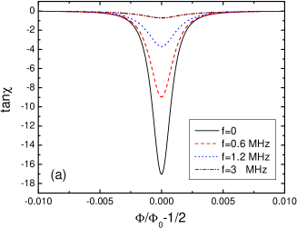
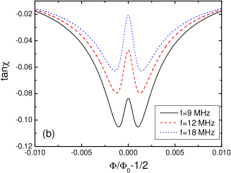
Figure 1: The dependence of the tank phase on the flux when under the influence of high frequency irradiation. $f=F/h$ is the power of irradiation in frequency units.

In conclusion, we propose a method to maintain the Rabi oscillations in a dissipative TLS by irradiating it with the two external sources. The first, high frequency source, which is tuned to the energy gap of the system, excites low frequency Rabi oscillations. The second, low frequency source, which is tuned to the frequency of the Rabi oscillations, causes the oscillations to persist. When applied to a readout of the flux qubit inductively coupled to a tank circuit, the method allows for the experimental determination of the relaxation and dephasing rates of the qubit.

References

• (1) I. I. Rabi, Phys. Rev. 51, 652 (1937).
• (2) Atomic and Molecular Beams: The State of The Art 2000, (Roger Compargue, ed.) Springer Verlag Telos, 2001.
• (3) J. M. Raimond, M. Brune, and S. Haroche, Rev. Mod. Phys. 73, 565 (2001).
• (4) A. N. Korotkov, cond-mat/0404696.
• (5) F. Bloch, Phys. Rev.105, 1206 (1957); A. G. Redfield, IBM J. Res. Dev. 1, 19 (1957).
• (6) L. Hartmann et al., Phys. Rev. E 61, R4687 (2000).
• (7) S. Saito et al., cond-mat/0403425 (2004).
• (8) Y. Makhlin, G. Schon, and A. Shnirman, Rev. Mod. Phys. 73, 357 (2001).
• (9) Y. Nakamura, Yu.A. Pashkin, and J.S. Tsai., Phys. Rev. Lett. 87, 246601 (2001).
• (10) D. Vion et al., Science 296, 886 (2002).
• (11) J.M. Martinis et al, Phys. Rev. Lett. 89, 117901 (2002).
• (12) I. Chiorescu et al.,Science 299, 1869 (2003).
• (13) D. V. Averin, cond-mat/0004364.
• (14) A.N. Korotkov Phys. Rev. B 64, 165310 (2001).
• (15) A.N. Korotkov and D.V. Averin, Phys. Rev. B 63, 115403 (2001).
• (16) E. Il’ichev et al., Phys. Rev. Lett. 91, 097906 (2003).
• (17) J.E. Mooij et al., Science 285, 1036 (1999).
• (18) T. P. Orlando et al., Phys. Rev. B 60, 15398 (1999).
• (19) A. Lupascu, C. J. P. M. Harmans, and J. E. Mooij, cond-mat/0410730.
• (20) A. Yu. Smirnov, Phys. Rev. B 68, 134514 (2003).
• (21) Ya. S. Greenberg et al., Phys. Rev B 66, 214525 (2002).
• (22) M. Grajcar et al., Phys. Rev. B 69, 060501(R) (2004).