Perfect quantum state transfer with randomly coupled quantum chains

Abstract

We suggest a scheme that allows arbitrarily perfect state transfer even in the presence of random fluctuations in the couplings of a quantum chain. The scheme performs well for both spatially correlated and uncorrelated fluctuations if they are relatively weak (say 5%). Furthermore, we show that given a quite arbitrary pair of quantum chains, one can check whether it is capable of perfect transfer by only local operations at the ends of the chains, and the system in the middle being a “black box”. We argue that unless some specific symmetries are present in the system, it will be capable of perfect transfer when used with dual-rail encoding. Therefore our scheme puts minimal demand not only on the control of the chains when using them, but also on the design when building them.

I Introduction

Recently, much interest has been devoted to quantum communication with quantum chains SB03 ; JOSEPH ; key-7 ; MCND+04 ; key-2 ; key-11 ; MYDL04 ; YUNG2 ; KARBACH ; key-1 ; TJO04 ; key-3 ; key-17 ; key-12 ; key-15 ; key-16 ; key-18 ; BBG ; MAURO ; key-6 ; PLENIO04 ; key-30 . The main spirit of these articles is that permanently coupled systems can be used for the transfer of quantum information with minimal control, that is, only the sending and the receiving parties can apply gates to the system, but the part of the chain interconnecting them cannot be controlled during the communication process. A scheme with less control is obviously impossible. The first proposals SB03 ; key-1 considered a regular spin chain with Heisenberg interactions. A physical implementation of this scheme was discussed in JOSEPH , and its channel capacity was derived in key-7 . Already in SB03 ; key-1 it was realized that such a transfer will, in general, not be perfect. The reason for the imperfect transfer is the dispersion of the information along the chain. This becomes worse as the chains get longer.

Since then, many very interesting methods have been developed to improve the fidelity of the transfer. One method is to use Hamiltonians with engineered couplings MCND+04 ; key-2 ; key-11 ; MYDL04 ; YUNG2 ; KARBACH such that the dispersed information will “refocus” at the receiving end of the chain. Another approach is to encode and decode the information using multiple spins TJO04 ; key-3 to form Gaussian wave packets (which have a lower dispersion). This has been generalized key-3 in an elegant way by using “phantom” spins such that a multiple-spin encoding can be achieved by only controlling two sending and receiving qubits. By using gapped systems key-17 ; key-12 ; key-15 ; key-16 , the intermediate spins are only virtually excited, and the transfer has a very high fidelity. Finally, in key-18 we have suggested a “dual-rail” encoding using two parallel quantum channels, achieving and arbitrarily perfect transfer. It was shown in BBG that such a protocol achieves arbitrarily perfect transfer for nearly any type of quantum chain, transforming a heavily dispersive dynamic into one that can be used for state transfer. In this scheme, not only the control needed during the transfer is minimized (no local access along the chains is needed), but also the control needed to design the system in the first place.

The main requirement for perfect transfer with dual-rail encoding as presented in the literature till date key-18 ; BBG is that two identical quantum chains have to be designed. While this is not so much a theoretical problem, for possible experimental realizations of the scheme JOSEPH the question naturally arises how to cope with slight asymmetries of the channels. The purpose of this paper is to demonstrate that in many cases, perfect state transfer with dual-rail encoding is possible for quantum chains with differing Hamiltonians.

By doing so, we also offer a solution to another and perhaps more general problem: if one implements any of the above schemes, the Hamiltonians will always be different from the theoretical ones by some random perturbation. This will lead to a decrease of fidelity in particular where specific energy levels were assumed (see key-19 for an analysis of fluctuations effecting the scheme MCND+04 ). Also in general, random systems can lead to a Anderson localization key-29 of the eigenstates (and therefore to low fidelity transport of quantum information). This problem can be avoided using the scheme described below. We will show numerically that the dual-rail scheme can still achieve arbitrarily perfect transfer for a uniformly coupled Heisenberg with random noise on the coupling strengths (both for the case of spatially correlated and uncorrelated fluctuations). Moreover, for any two quantum chains, we show that Bob and Alice can check whether their system is capable of dual-rail transfer without directly measuring their Hamiltonians or local properties of the system along the chains but by only measuring their part of the system.

II Conclusive transfer

By “conclusive transfer”, we mean that the receiver has a certain probability for obtaining the perfectly transferred state, and some way of checking whether this has happened. Conclusive transfer is more valuable than simple state transfer with the same fidelity, because errors are detected and memory effects WERNER are unimportant if the transfer was successfull. A single spin-$1/2$ quantum chain could however not be used for conclusive transfer, because any measurement can easily destroy the unknown quantum state that is being transferred. The simplest quantum chain for conclusive transfer is a system consisting of two uncoupled quantum chains $(1)$ and $(2)$, as shown in Fig. 1. The chains are described by the two Hamiltonians $H^{(1)}$ and $H^{(2)}$ acting on the corresponding Hilbert spaces $\mathcal{H}_{1}$ and $\mathcal{H}_{2}.$ The total Hamiltonian is thus

$$H=H^{(1)}\otimes I^{(2)}+I^{(1)}\otimes H^{(2)},$$ (1)

and the time evolution operator factorizes as

$$U(t) = \exp\left(-iHt\right)$$ (2)

$$= \exp\left(-iH^{(1)}t\right)\otimes\exp\left(-iH^{(2)}t\right).$$ (3)

For the moment, we assume that both chains have equal length $N$, but it will become clear in Section IV that this is not a requirement of our scheme. Like in key-18 ; BBG , we assume that the quantum chains consist of qubits and that both Hamiltonians commute with the z-component of the total spin of chains,

$$\left[H^{(1)},\sum_{i=1}^{N}\sigma_{z}^{(1)}\right]=\left[H^{(2)},\sum_{i=1}^{N}\sigma_{z}^{(2)}\right]=0.$$ (4)

It then follows that the state

$$\left|\mathbf{0}\right\rangle^{(i)}\equiv\left|00\ldots 0\right\rangle^{(i)}$$ (5)

is an eigenstate of $H^{(i)}$ and that the dynamics of an initial state of the form

$$\left|\mathbf{1}\right\rangle^{(i)}\equiv\left|10\ldots 0\right\rangle^{(i)}$$ (6)

is restricted to the subspace of single excitations,

$$\left|\mathbf{m}\right\rangle^{(i)}\equiv\left|0\ldots 0\begin{array}[t]{c}1\\ m\textrm{th}\end{array}0\ldots 0\right\rangle^{(i)}\quad(1\leq m\leq N).$$ (7)

In the following, we will omit all indexes and write the states of the full Hilbert space $\mathcal{H}_{1}\otimes\mathcal{H}_{2}$ as

$$\left|\mathbf{m,n}\right\rangle\equiv\left|\mathbf{m}\right\rangle^{(1)}\otimes\left|\mathbf{n}\right\rangle^{(2)}.$$ (8)

We assume that the sender, Alice, has full access to the first qubit of each chain, and that the receiver, Bob, has full access to the last qubit of each chain. With “full access” we mean that they can perform a two-qubit gate (say, a CNOT), and arbitrary single-qubit operations. Bob also needs the ability to perform single-qubit measurements.

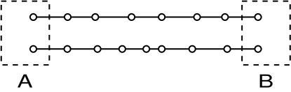
Figure 1: Two quantum chains interconnecting $A$ and $B$. Control of the systems is only possible at the two qubits of either end.

Initially, Alice encodes the state as

$$\alpha\left|\mathbf{0,1}\right\rangle+\beta\left|\mathbf{1,0}\right\rangle.$$ (9)

This is a superposition state of an excitation in the first qubit of the first chain with an excitation in the first qubit of the second chain. The state will evolve in

$$\sum_{n=1}^{N}\left\{\alpha g_{n,1}(t)\left|\mathbf{0,n}\right\rangle+\beta f_{n,1}(t)\left|\mathbf{n,0}\right\rangle\right\}.$$ (10)

Note that there is only one excitation in the system. The probability amplitudes are given by

$$f_{n,1}(t) \equiv \left\langle\mathbf{n,0}\left|U(t)\right|\mathbf{1,0}\right\rangle$$ (11)

$$g_{n,1}(t) \equiv \left\langle\mathbf{0,n}\left|U(t)\right|\mathbf{0,1}\right\rangle.$$ (12)

In key-18 , these functions were identical. For differing chains this is no longer the case. We may, however, find a time $t_{1}$ such that the modulus of their amplitudes at the last spins are the same (see Fig. 2),

$$g_{N,1}(t_{1})=e^{i\phi_{1}}f_{N,1}(t_{1}).$$ (13)

Figure 2: The absolute values of the transition amplitudes $f_{N,1}(t)$ and $g_{N,1}(t)$ for two Heisenberg chains of length $N=10$. The couplings strengths of both chains were chosen randomly from the interval $\left[0.8J,1.2J\right].$ The circles show times where Bob can perform measurements without gaining information on $\alpha$ and $\beta.$

At this time, the state (10) can be written as

$$\sum_{n=1}^{N-1}\left\{\alpha g_{n,1}(t_{1})\left|\mathbf{0,n}\right\rangle+\beta f_{n,1}(t_{1})\left|\mathbf{n,0}\right\rangle\right\}+$$

$$f_{N,1}(t_{1})\left\{e^{i\phi_{1}}\alpha\left|\mathbf{0,N}\right\rangle+\beta\left|\mathbf{N,0}\right\rangle\right\}.$$ (14)

Bob decodes the state by applying a CNOT gate on his two qubits, with the first qubit as the control bit. The state thereafter is

$$\sum_{n=1}^{N-1}\left\{\alpha g_{n,1}(t_{1})\left|\mathbf{0,n}\right\rangle+\beta f_{n,1}(t_{1})\left|\mathbf{n,0}\right\rangle\right\}+$$

$$f_{N,1}(t_{1})\left\{e^{i\phi_{1}}\alpha\left|\mathbf{0}\right\rangle^{(1)}+\beta\left|\mathbf{N}\right\rangle^{(1)}\right\}\otimes\left|\mathbf{N}\right\rangle^{(2)}.$$ (15)

Bob then measures his second qubit. Depending on the outcome of this measurement, the systems will either be in the state

$$\frac{1}{\sqrt{p_{1}}}\sum_{n=1}^{N-1}\left\{\alpha g_{n,1}(t_{1})\left|\mathbf{0,n}\right\rangle+\beta f_{n,1}(t_{1})\left|\mathbf{n,0}\right\rangle\right\}$$ (16)

or in

$$\left\{e^{i\phi_{1}}\alpha\left|\mathbf{0}\right\rangle^{(1)}+\beta\left|\mathbf{N}\right\rangle^{(1)}\right\}\otimes\left|\mathbf{N}\right\rangle^{(2)},$$ (17)

where $p_{1}=1-\left|f_{N,1}(t_{1})\right|^{2}=1-\left|g_{N,1}(t_{1})\right|^{2}$ is the probability that Bob has not received the state. The state (17) corresponds to the correctly transferred state with a known phase error (which can be corrected by Bob using a simple phase gate). If Bob finds the system in the state (16), the transfer has been unsuccessful, but the information is still in the chain. We thus see that conclusive transfer is still possible with randomly coupled chains as long as the requirement (13) is met. This requirement will be further discussed and generalized in the next section.

III Arbitrarily perfect transfer

If the transfer was unsuccessful, the state (16) will evolve further, offering Bob further opportunities to receive Alice’s message. For identical quantum chains, this must ultimately lead to a success for any reasonable Hamiltonian BBG . For differing chains, this is not necessarily the case, because measurements are only allowed at times where the probability amplitude at the end of the chains are equal, and there may be systems where this is never the case. In this section, we will develop a criterion that generalizes Eq. (13) and allows to check numerically whether a given system is capable of arbitrarily perfect state transfer.

The quantity of interest for conclusive state transfer is the joint probability $\mathcal{P}(l)$ that after having checked $l$ times, Bob still has not received the proper state at his ends of the chain. Optimally, this should approach zero if $l$ tends to infinity. In order to derive an expression for $\mathcal{P}(l),$ let us assume that the transfer has been unsuccessful for $l-1$ times with time intervals $t_{i}$ between the the $i$th and the $(i-1)$th measurement, and calculate the probability of failure at the $l$th measurement. In a similar manner, we assume that all the $l-1$ measurements have met the requirement of conclusive transfer (that is, Bob’s measurements are unbiased with respect to $\alpha$ and $\beta$) and derive the requirements for the $l$th measurement.

To calculate the probability of failure for the $l$th measurement, we need to take into account that Bob’s measurements disturb the unitary dynamics of the chain. If the state before a measurement with the outcome “failure” is $\left|\psi\right\rangle,$ the state after the measurement will be

$$\frac{1}{\sqrt{p_{l}}}Q\left|\psi\right\rangle,$$ (18)

where $Q$ is the projector

$$Q=I-\left|\mathbf{0,N}\right\rangle\left\langle\mathbf{0,N}\right|-\left|\mathbf{N,0}\right\rangle\left\langle\mathbf{N,0}\right|,$$ (19)

and $p_{l}$ is the probability of failure at the $l$th measurement. The dynamics of the chain is alternating between unitary and projective, such that the state before the $l$th measurement is given by

$$\frac{1}{\sqrt{\mathcal{P}(l-1)}}\prod_{i=1}^{l}\left\{U(t_{i})Q\right\}\left\{\alpha\left|\mathbf{1,0}\right\rangle+\beta\left|\mathbf{0,1}\right\rangle\right\},$$ (20)

where we have used that

$$Q\left\{\alpha\left|\mathbf{1,0}\right\rangle+\beta\left|\mathbf{0,1}\right\rangle\right\}=\alpha\left|\mathbf{1,0}\right\rangle+\beta\left|\mathbf{0,1}\right\rangle$$ (21)

for the first factor $i=1$, and

$$\mathcal{P}(l-1)=\prod_{i=1}^{l-1}p_{l}.$$ (22)

Note that the operators in (20) do not commute and that the time ordering of the product (the index $i$ increases from right to left) is important. The probability that there is an excitation at the $N$th site of either chain is given by

$$\frac{1}{\mathcal{P}(l-1)}\left\{\left|\alpha\right|^{2}\left|F(l)\right|^{2}+\left|\beta\right|^{2}\left|G(l)\right|^{2}\right\},$$ (23)

with

$$F(l)\equiv\left\langle\mathbf{N,0}\right|\prod_{i=1}^{l}\left\{U(t_{i})Q\right\}\left|\mathbf{1,0}\right\rangle,$$ (24)

and

$$G(l)\equiv\left\langle\mathbf{0,N}\right|\prod_{i=1}^{l}\left\{U(t_{i})Q\right\}\left|\mathbf{0,1}\right\rangle.$$ (25)

Bob’s measurements are therefore unbiased with respect to $\alpha$ and $\beta$ if and only if

$$\left|F(l)\right|=\left|G(l)\right|\quad\forall l.$$ (26)

In this case, the state can still be transferred conclusively (up to a known phase). The probability of failure at the $l$th measurement is given by

$$p_{l}=1-\frac{\left|F(l)\right|^{2}}{\mathcal{P}(l-1)}.$$ (27)

We will show in the Appendix that the condition (26) is equivalent to

$$\left\|\prod_{i=1}^{l}\left\{U(t_{i})Q\right\}\left|\mathbf{1,0}\right\rangle\right\|=\left\|\prod_{i=1}^{l}\left\{U(t_{i})Q\right\}\left|\mathbf{0,1}\right\rangle\right\|\quad\forall l,$$ (28)

and that the joint probability of failure is simply

$$\mathcal{P}(l)=\left\|\prod_{i=1}^{l+1}\left\{U(t_{i})Q\right\}\left|\mathbf{1,0}\right\rangle\right\|^{2}.$$ (29)

It may look as if Eq. (28) was a complicated multi-time condition for the measuring times $t_{i}$, that becomes increasingly difficult to fulfill with a growing number of measurements. This is not the case. If proper measuring times have been found for the first $l-1$ measurements, a trivial time $t_{l}$ that fulfills Eq. (28) is $t_{l}=0.$ In this case, Bob measures immediately after the $(l-1)$th measurement and the probability amplitudes on his ends of the chains will be equal - but zero (a useless measurement). But since the left and right hand side of Eq. (28) when seen as functions of $t_{l}$ are both quasi-periodic functions with initial value zero, it is likely that they intersect many times, unless the system has some specific symmetry or the systems are completely different. Furthermore, for the $l$th measurement, Eq. (28) is equivalent to

$$\left\|QU(t_{l})\left|\xi\right\rangle\right\|\equiv\left\|QU(t_{l})\left|\zeta\right\rangle\right\|$$ (30)

with

$$\left|\xi\right\rangle=Q\prod_{i=1}^{l-1}U(t_{i})Q\left|\mathbf{1,0}\right\rangle$$ (31)

and

$$\left|\zeta\right\rangle=Q\prod_{i=1}^{l-1}U(t_{i})Q\left|\mathbf{0,1}\right\rangle.$$ (32)

From this we can see that if the system is ergodic, the condition for conclusive transfer is fulfilled at many different times.

Note that we do not claim at this point that any pair of chains will be capable of arbitrary perfect transfer. We will discuss in the next system how one can check this for a given system by performing some simple experimental tests.

IV Tomography

Suppose someone gives you two different experimentally designed spin chains. It may seem from the above that knowledge of the full Hamiltonian of both chains is necessary to check how well the system can be used for state transfer. This would be a very difficult task, because we would need access to all the spins along the channel to measure all the parameters of the Hamiltonian. In fact by expanding the projectors in Eq. (28) one can easily see that the only matrix elements of the evolution operator which are relevant for conclusive transfer are

$$f_{N,1}(t) = \left\langle\mathbf{N,0}\right|U(t)\left|\mathbf{1,0}\right\rangle$$ (33)

$$f_{N,N}(t) = \left\langle\mathbf{N,0}\right|U(t)\left|\mathbf{N,0}\right\rangle$$ (34)

$$g_{N,1}(t) = \left\langle\mathbf{0,N}\right|U(t)\left|\mathbf{0,1}\right\rangle$$ (35)

$$g_{N,N}(t) = \left\langle\mathbf{0,N}\right|U(t)\left|\mathbf{0,N}\right\rangle.$$ (36)

Physically, this means that the only relevant properties of the system are the transition amplitudes to arrive at Bob’s ends and to stay there. The modulus of $f_{N,1}(t)$ and $f_{N,N}(t)$ can be measured by initialising the system in the states $\left|\mathbf{1,0}\right\rangle$ and $\left|\mathbf{N,0}\right\rangle$ and then performing a reduced density matrix tomography at Bob’s site at different times $t$, and the complex phase of these functions is obtained by initialising the system in $\left(\left|\mathbf{0,0}\right\rangle+\left|\mathbf{1,0}\right\rangle\right)/\sqrt{2}$ and $\left(\left|\mathbf{0,0}\right\rangle+\left|\mathbf{N,0}\right\rangle\right)/\sqrt{2}$ instead. In the same way, $g_{N,1}(t)$ and $g_{N,N}(t)$ are obtained. All this can be done in the spirit of minimal control at the sending and receiving ends of the chain only, and needs to be done only once. It is interesting to note that the dynamics in the middle part of the chain is not relevant at all. It is a “black box” that may involve even completely different interactions, number of spins, etc. (see Fig. 3).

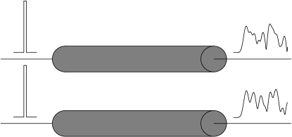
Figure 3: The relevant properties for conclusive transfer can be determined by measuring the response of the two systems at their ends only.

Once the transition amplitudes (Equations (33)-(36)) are known, one can search numerically for optimized measurement times $t_{i}$ using Eq. (29) and the condition from Eq. (28).

One weakness of the scheme described here is that the times at which Bob measures have to be very precise, because otherwise the measurements will not be unbiased with respect to $\alpha$ and $\beta.$ This demand can be relaxed by measuring at times where not only the probability amplitudes are similar, but also their slope (see Fig. 2). The computation of these optimal timings for a given system may be complicated, but they only need to be done once.

V Numerical Examples

In this section, we show some numerical examples for two chains with Heisenberg couplings $J$ which are fluctuating. The Hamiltonians of the chains are given by

$$H^{(1)} = \sum_{n=1}^{N-1}J(1+\delta_{n}^{(1)})\vec{\sigma}_{n}^{(1)}\cdot\vec{\sigma}_{n+1}^{(1)},$$ (37)

$$H^{(2)} = \sum_{n=1}^{N-1}J(1+\delta_{n}^{(2)})\vec{\sigma}_{n}^{(2)}\cdot\vec{\sigma}_{n+1}^{(2)},$$ (38)

where $\delta_{n}^{(i)}$ uniformly distributed random numbers from the interval $\left[-\Delta,\Delta\right].$ We have considered two different cases: in the first case, the $\delta_{n}^{(i)}$ are completey uncorrelated (i.e. independent for both chains and all sites along the chain). In the second case, we have taken into account a spacial correlation of the signs of the $\delta_{n}^{(i)}$ along each of the chains, while still keeping the two chains uncorrelated. For both cases, we find that arbitrarily perfect transfer remains possible except for some very rare realisations of the $\delta_{n}^{(i)}.$

Because measurements must only be taken at times which fulfill the condition (28) and these times usually do not coincidence with the optimal probability of finding an excitation at the ends of the chains, it is clear that the probability of failure at each measurement will in average be higher than for chains without fluctuations. Therefore, a bigger number of measurements have to be performed in order to achieve the same probability of success. The price for noisy couplings is thus a longer transmission time and a higher number of gating operations at the receiving end of the chains. Some averaged values are given in Table 1.

	$\Delta=0$	$\Delta=0.01$	$\Delta=0.03$	$\Delta=0.05$	$\Delta=0.1$
$t$$\left[\frac{\hbar}{J}\right]$	$377$	$524\pm 27$	$694\pm 32$	$775\pm 40$	$1106\pm 248$
$M$	$28$	$43\pm 3$	$58\pm 3$	$65\pm 4$	$110\pm 25$

Table 1: The total time $t$ and the number of measurements $M$ needed to achieve a probability of success of $99$% for different fluctuation strengths $\Delta$ (uncorrelated case). Given is the statistical mean and the standard deviation. The length of the chain is $N=20$ and the number of random samples is $10.$ For strong fluctuations $\Delta=0.1$, we also found particular samples where the success probability could not be achieved within the time range searched by the algorithm.

for the Heisenberg chain with uncorrelated coupling fluctuations.

For the case were the signs of the $\delta_{n}^{(i)}$ are correlated, we have used the same model as in key-19 , introducing the parameter $c$ such that

$$\delta_{n}^{(i)}\delta_{n-1}^{(i)}>0\qquad\textrm{with propability }c,$$ (39)

and

$$\delta_{n}^{(i)}\delta_{n-1}^{(i)}<0\qquad\textrm{with propability }1-c.$$ (40)

For $c=1$ ($c=0)$ this corresponds to the case where the signs of the couplings are completely correlated (anticorrelated). For $c=0.5$ one recovers the case of uncorrelated couplings. We can see from the numerical results in Table 2 that arbitrarily perfect transfer is possible for the whole range of $c.$

	$c=0$	$c=0.1$	$c=0.3$	$c=0.7$	$c=0.9$	$c=1$
$t$$\left[\frac{\hbar}{J}\right]$	$666\pm 20$	$725\pm 32$	$755\pm 41$	$797\pm 35$	$882\pm 83$	$714\pm 41$
$M$	$256\pm 2$	$62\pm 3$	$65\pm 4$	$67\pm 4$	$77\pm 7$	$60\pm 4$

Table 2: The total time $t$ and the number of measurements $M$ needed to achieve a probability of success of $99$% for different correlations $c$ between the couplings (see Eq. (39) and Eq. (40)). Given is the statistical mean and the standard deviation for a fluctuation strength of $\Delta=0.05$. The length of the chain is $N=20$ and the number of random samples is $20.$

For $\Delta=0$, we know from key-18 that the time to transfer a state with probability of failure $P$ scales as

$$t(P)=\frac{0.33\hbar N^{1.6}}{J}\left|\ln P\right|.$$ (41)

If we want obtain a similar formula in the presence of noise, we have can perform a fit to the exact numerical data. For uncorrelated fluctuations of $\Delta=0.05,$ this is shown in Fig. 4. The best fit is given by

$$t(P)=\frac{0.2\hbar N^{1.9}}{J}\left|\ln P\right|.$$ (42)

We conclude that weak fluctuations (say up to $5$%) in the coupling strengths do not deteriorate the performance of our scheme much for the chain lengths considered. Both the transmission time and the number of measurements raise, but still in a reasonable way (cf. Table 1 and Eq. (4)). For larger fluctuations, the scheme is still applicable in principle, but the amount of junk (i.e. chains not capable of arbitrary perfect transfer) may get too large.

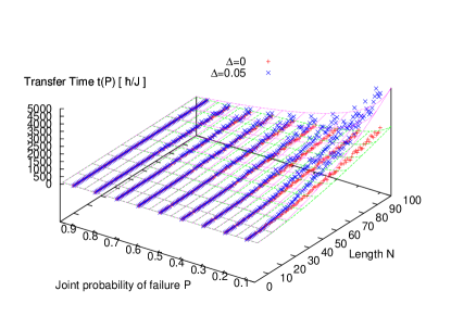
Figure 4: Time $t$ needed to transfer a state with a given joint probability of failure $P$ across a chain of length $N$ with uncorrelated fluctuations of $\Delta=0.05$ and without fluctuations ($\Delta=0$ ). The points denote exact numerical data, and the fits are given by Eq. (41) and Eq. (42).

VI Conclusions

We have shown that in many cases, it is possible to perfectly transfer an unknown quantum state along a pair of quantum chains even if their coupling is to some amount random. This is achieved using a dual-rail encoding combined with measurements at the receiving end of the chains. Since any scheme for quantum communication will suffer from some imperfections when implemented, the dual-rail is a powerful tool to overcome the decrease of fidelity.

This work was supported by the UK Engineering and Physical Sciences Research Council through the grant GR/S62796/01 and the QIPIRC.

Appendix

We first use Eq. (22) and (27) to obtain

$$\mathcal{P}(l)=\mathcal{P}(l-1)-\left|F(l)\right|^{2},$$ (43)

or, using $\mathcal{P}(0)=1$,

$$\mathcal{P}(l) = 1-\sum_{k=1}^{l}\left|F(k)\right|^{2}.$$ (44)

If we introduce

$$v(l) \equiv \left\|\prod_{i=1}^{l}\left\{U(t_{i})Q\right\}\left|\mathbf{1,0}\right\rangle\right\|^{2},$$ (45)

$$w(l) \equiv \left\|\prod_{i=1}^{l}\left\{U(t_{i})Q\right\}\left|\mathbf{0,1}\right\rangle\right\|^{2},$$ (46)

then we can write

$$\left|F(l)\right|^{2}=$$ (47)

$$= \left\langle\mathbf{1,0}\right|\left(\prod_{i=1}^{l}\left\{U(t_{i})Q\right\}\right)^{\dagger}\left|\mathbf{N,0}\right\rangle\left\langle\mathbf{N,0}\right|\prod_{i=1}^{l}\left\{U(t_{i})Q\right\}\left|\mathbf{1,0}\right\rangle$$

$$= v(l)-\left\langle\mathbf{1,0}\right|\left(\prod_{i=1}^{l}\left\{U(t_{i})Q\right\}\right)^{\dagger}Q\prod_{i=1}^{l}\left\{U(t_{i})Q\right\}\left|\mathbf{1,0}\right\rangle$$

$$= v(l)-\left\|\prod_{i=1}^{l}Q\left\{U(t_{i})Q\right\}\left|\mathbf{1,0}\right\rangle\right\|^{2}$$

$$= v(l)-v(l+1),$$

where we have used

$$\left|\mathbf{N,0}\right\rangle\left\langle\mathbf{N,0}\right| = 1-Q-\left|\mathbf{0,N}\right\rangle\left\langle\mathbf{0,N}\right|,$$ (48)

$$Q^{2} = Q,$$ (49)

and the fact that the unitary matrix $U(t_{l+1})$ does not change the norm of a vector. The same calculation can be done for $\left|G(l)\right|^{2}$ such that

$$\left|G(l)\right|^{2} = w(l)-w(l+1).$$ (50)

If we want to have $\left|F\right|$ and $\left|G\right|$ matching for all $l$, we need to have

$$w(l)=v(l)\quad\forall l,$$ (51)

or

$$\left\|\prod_{i=1}^{l}\left\{U(t_{i})Q\right\}\left|\mathbf{1,0}\right\rangle\right\|=\left\|\prod_{i=1}^{l}\left\{U(t_{i})Q\right\}\left|\mathbf{0,1}\right\rangle\right\|\quad\forall l.$$ (52)

The joint probability of failure is given by

$$\mathcal{P}(l) = 1-\sum_{k=1}^{l}\left|F(k)\right|^{2}$$ (53)

$$= 1-\sum_{k=1}^{l}v(k)-v(k+1)$$ (54)

$$= v(l+1)$$ (55)

$$= \left\|\prod_{i=1}^{l+1}Q\left\{U(t_{i})Q\right\}\left|\mathbf{1,0}\right\rangle\right\|^{2}.$$ (56)

References

- (1) S. Bose, Phys. Rev. Lett. 91, 207901 (2003)
- (2) V. Subrahmanyam, Phys. Rev. A 69, 034304 (2004)
- (3) A. Romito, R. Fazio, C. Bruder, quant-ph/0408057.
- (4) V. Giovannetti and R. Fazio, quant-ph/0405110.
- (5) M. Christandl, N. Datta, A. Ekert and A. J. Landahl, Phys. Rev. Lett. 92, 187902 (2004)
- (6) C. Albanese, M. Christandl, N. Datta and A. Ekert, Phys. Rev. Lett. 93, 230502 (2004)
- (7) M. Christandl, N. Datta, T. C. Dorlas, A. Ekert, A. Kay and A. J. Landahl, quant-ph/0411020
- (8) MH Yung, DW Leung and S. Bose, Quant. Inf. & Comp. 4, 174 (2004)
- (9) MH Yung and S. Bose, quant-ph/0407212
- (10) P. Karbach and J. Stolze, quant-ph/0501007
- (11) T. J. Osborne and N. Linden, Phys. Rev. A 69, 052315 (2004)
- (12) H. L. Haselgrove, quant-ph/0404152.
- (13) M.B. Plenio, F. L. Semiao, New. J. Phys. 7, 73 (2005)
- (14) Y.Li, T.Shi, B.Chen, Z.Song, C.P.Sun, Phys. Rev. A 71, 022301
- (15) T. Shi, Ying Li, Z. Song, C. P. Sun, quant-ph/0408152
- (16) Z. Song, C. P. Sun, quant-ph/0412183
- (17) D. Burgarth and S. Bose, quant-ph/0406112
- (18) D. Burgarth, S. Bose and V. Giovannetti, quant-ph/0410175
- (19) M. Paternostro, G.M. Palma, M.S. Kim and G. Falci, quant-ph/0407058
- (20) L. Amico, A. Osterloh, F. Plastina, R. Fazio and G. M. Palma, Phys. Rev. A 69, 022304 (2004)
- (21) M.B. Plenio, J. Hartley and J. Eisert, New J. of Phys. 6, 36 (2004).
- (22) J. Eisert, M.B. Plenio, S. Bose and J. Hartley, Phys. Rev. Lett 93, 190402 (2004)
- (23) G. De Chiara, D. Rossini, S. Montangero, R. Fazio, quant-ph/0502148
- (24) P. W. Anderson, Phys. Rev. 109, 1492 (1958)
- (25) D. Kretschmann, R. F. Werner, quant-ph/0502106