The Sources of Intergalactic Metals

Abstract

We study the clustering properties of metals in the intergalactic medium (IGM) as traced by 619 C iv and 81 Si iv absorption components with $N\geq 10^{12}$ cm^-2 and 316 Mg ii and 82 Fe ii absorption components with $N\geq 10^{11.5}$ cm^-2 in 19 high signal-to-noise (60-100 per pixel), high resolution ($R=45000$) quasar spectra. C iv and Si iv trace each other closely and their line-of-sight correlation functions $\xi(v)$ exhibit a steep decline at large separations and a flatter profile below $\approx 150$ km s^-1, with a large overall bias. These features do not depend on absorber column densities, although there are hints that the overall amplitude of $\xi_{{\rm C\,\sc iv}}$ increases with time over the redshifts range detected (1.5-3). Carrying out a detailed smoothed particle hydrodynamic simulation ($2\times 320^{3}$, $57$ Mpc³ comoving), we show that the C iv correlation function can not be reproduced by models in which the IGM metallicity is a constant or a local function of overdensity ($Z\propto\Delta^{2/3}$). However, the properties of $\xi_{{\rm C\,\sc iv}}(v)$ are generally consistent with a model in which metals are confined within bubbles with a typical radius $R_{s}$ about sources of mass $\geq M_{s}.$ We derive best-fit values of $R_{s}\approx 2$ comoving Mpc and $M_{s}\approx 10^{12}\,{\rm M_{\odot}}$ at $z=3$. Our lower redshift ($0.5-2$) measurements of the Mg ii and Fe ii correlation functions also uncover a steep decline at large separations and a flatter profile at small separations, but the clustering is even higher than in the $z=$1.5-3 measurements, and the turn-over is shifted to somewhat smaller distances $\approx 75$ km s^-1. Again these features do not change with column density, but there are hints that the amplitudes of $\xi_{{\rm Mg\,\sc ii}}(v)$ and $\xi_{{\rm Fe\,\sc ii}}(v)$ increase with time. We describe an analytic “bubble” model for these species, which come from regions that are too compact to be accurately simulated numerically, deriving best-fit values of $R_{s}\approx 2.4$ Mpc and $M_{s}\approx 10^{12}\,{\rm M_{\odot}}.$ Equally good analytic fits to all four species are found in a similarly biased high-redshift enrichment model in which metals are placed within $2.4$ comoving Mpc of $M_{s}\approx 3\times 10^{9}$ sources at $z=7.5.$

1 Introduction

Pollution is ubiquitous. Even in the tenuous intergalactic medium (IGM), quasar (QSO) absorption line studies have encountered heavy elements in all regions in which they were detectable (Tytler et al. 1995; Songaila & Cowie 1996). Such analyses were limited at first to somewhat overdense regions of space, traced by Ly$\alpha$ clouds with column densities $N_{\rm HI}\geq 10^{14.5}$ cm^-2. Here measurements of $N_{\rm CIV}/N_{\rm HI}$ indicated that typically $[C/H]\simeq-2.5$ at $z\simeq 3$, with an order of magnitude scatter (Hellsten et al. 1997; Rauch, Haehnelt, & Steinmetz 1997).

Pushing into more tenuous regions, statistical methods have shown that unrecognized weak absorbers must be present in order to reproduce the global C iv optical depth (Ellison et al. 2000), and that a minimum IGM metallicity of approximately $3\times 10^{-3}Z_{\odot}$ was already in place at $z=5$ (Songaila 2001; hereafter S01). While the filling factor of metals in such tenuous structures is an object of intense investigation and debate (Schaye et al. 2000; Petitjean 2001; Bergeron et al. 2002; Carswell et al. 2002; Simcoe et al. 2002; Pettini et al. 2003; Schaye et al. 2003; Aracil et al. 2004) their very existence has profound cosmological implications.

As the presence of metals increases the number of lines available for radiative cooling, even modest levels of enrichment can greatly enhance the cooling rate (e.g. Sutherland & Dopita 1993), which has the potential to accelerate the formation of massive ($\lower 2.15277pt\hbox{$\;\buildrel>\over{\sim}\;$}10^{12}\,{\rm M_{\odot}}$) galaxies (e.g. Thacker, Scannapieco & Davis 2002). Furthermore, significant preenrichment is necessary to reproduce the abundances of G-dwarf stars in the Milky Way (e.g. van de Bergh 1962; Schmidt 1963) and nearby galaxies (e.g. Thomas, Greggio, & Bender 1999).

Similarly, the violent events that propelled heavy elements into the space between galaxies have important implications for the thermal and velocity structure of the IGM (e.g. Tegmark, Silk, & Evrard 1993; Gnedin & Ostriker 1997; Cen & Bryan 2001). Outflows energetic enough to eject metals from the potential wells of dwarf galaxies, for example, would have exerted strong feedback effects on nearby objects (Thacker, Scannapieco, & Davis 2002). In this case the winds impinging on pre-virialized overdense regions would have been sufficiently powerful to strip the baryons from their associated dark matter, greatly reducing the number of $\lower 2.15277pt\hbox{$\;\buildrel<\over{\sim}\;$}10^{10}\,{\rm M_{\odot}}$ galaxies formed (Scannapieco, Ferrara, & Broadhurst 2000; Sigward, Ferrara, & Scannapieco 2005).

Yet despite their many consequences, the details of how metals came to enrich the IGM are unclear. While numerous starburst-driven outflows have been observed at $z=3$ (Pettini et al. 2001) and in lensed galaxies at $4\lower 2.15277pt\hbox{$\;\buildrel<\over{\sim}\;$}z\lower 2.15277pt\hbox{$\;\buildrel<\over{\sim}\;$}5$ (Frye, Broadhurst, & Benitez 2002), it is unclear whether these objects are responsible for the majority of cosmological enrichment. In fact a variety of theoretical arguments suggest that such galaxies represent only the tail end of a larger population of smaller “pre-galactic” starbursts that mostly formed at much higher redshifts (Madau, Ferrara, & Rees 2001; Scannapieco, Ferrara, & Madau 2002). On the other hand, active galactic nuclei are observed to host massive outflows (Begelman, Blandford, & Rees 1984; Weyman 1997), whose contribution from less luminous objects at intermediate redshifts remains unknown (e.g. Fan et al. 2001). The impact of such lower-redshift events on the IGM is also hinted at by the “stirring” of C iv systems observed in studies of lensed QSO pairs (Rauch, Sargent, & Barlow 2001). Finally, a number of theoretical studies suggest that primordial, metal-free stars may have been very massive (e.g. Bromm et al. 2001; Schneider et al. 2002), resulting in a large number of tremendously powerful pair-production supernovae, which distributed metals into the IGM at extremely early redshifts $\lower 2.15277pt\hbox{$\;\buildrel>\over{\sim}\;$}15$ (Bromm 2003; Norman, O’Shea, & Paschos 2004).

While perhaps the main feature shared by such scenarios is their dependence on a poorly-understood population of presently undetectable objects, this assessment paints an overly bleak picture. Regardless of which objects enriched the IGM, it is clear that they must have formed in the densest regions of space, regions that are far more clustered than the overall dark matter distribution. Furthermore this “geometrical biasing” is a systematic function of the masses of these structures, an effect that has been well studied analytically and numerically (e.g. Kaiser 1984; Jing 1999). Thus the observed large-scale clustering of metal absorbers encodes valuable information about the masses of the objects from which they were ejected. Likewise, as the maximal extent of each enriched region is directly dependent on the velocity at which the metals were dispersed, measurements of the small-scale clustering of these absorbers are likely to constrain the energetics of their sources.

Previous studies of the two-point correlation function of C iv components have shown that they cluster strongly on velocity scales up to 500 km s^-1 (Sargent et al. 1980, Steidel 1990, Petitjean & Bergeron 1994, Rauch et al. 1996). It has often been suggested that the clustering signal reflects a combination of (i) relative motions of clouds within a galactic halo and (ii) galaxy clustering. More recently Boksenberg, Sargent, & Rauch (2003; hereafter BSR03) have gathered a sample of 908 C iv absorber components clumped into 199 systems in the redshift range 1.6 $<$ $z$ $<$ 4.4 identified in the Keck spectra of nine QSOs. They conclude that most of the signal is due to the clustering of components within each system, where a system is defined as a set of components that is “well-separated” from its neighbours as identified by the observer. In this case almost all the systems extend less than 300 km s^-1 and most extend less than 150 km s^-1. They did not observe clustering between systems on the larger scales expected for galaxy clustering, although they concluded from their measurements of component clustering and ionisation balance that each system was closely associated with a galaxy.

In Pichon et al. (2003; hereafter Paper I) we used 643 C iv and 104 Si iv absorber components, measured by an automated procedure in 19 high signal-to-noise quasar spectra, to place strong constraints on the number and spatial distribution of intergalactic metals at intermediate redshifts ($2\leq z\leq 3$). In this work, we showed that the correlation functions of intergalactic C iv and Si iv could be understood in terms of the clustering of metal bubbles of a typical comoving radius $R_{s}$ around sources whose biased clustering was parameterized by a mass $M_{s}$. A similar picture was also put forward in BSR03, but in our case significant large-scale clustering, similar to that seen in galaxies, was observed.

In this paper we extend the analysis in Paper I in three important ways. First we carry out a more detailed study of the physical properties of C iv and Si iv absorbers and the relationship between local quantities and the overall spatial distribution. Second, we carry out a similar analysis of Mg ii and Fe ii absorbers in our observational sample, which probe the IGM in a somewhat lower redshift range. Finally, we replace our dark-matter only modeling of Paper I with a full-scale smoothed-particle hydrodynamical simulation. We then generate simulated metal-line spectra by painting bubbles of metals directly onto the gas distribution at $z\geq 2$. By analyzing the resulting spectra with the same automated procedure applied to the measured data-set, we are able to place our models and observations on the same footing, drawing important constraints on the sources of metals. Motivated by measurements of the cosmic microwave background, the number abundance of galaxy clusters, and high-redshift supernovae (e.g. Spergel et al. 2003; Eke et al. 1996; Perlmutter et al. 1999) we adopt cosmological parameters of $h=0.7$, $\Omega_{m}$ = 0.3, $\Omega_{\Lambda}$ = 0.7, $\Omega_{b}=0.044$, throughout this investigation where $h$ is the Hubble Constant in units of 100 km s^-1 Mpc^-1 and $\Omega_{m}$, $\Omega_{\Lambda}$, and $\Omega_{b}$ are the total matter, vacuum, and baryonic densities in units of the critical density, $\rho_{\rm crit}.$

The structure of this work is as follows. In §2 we summarize the properties of our data set and reduction methods. In §3 we present the number densities of C iv, Si iv, Mg ii, and Fe ii, and estimate the cosmological densities of these species. In §4 we study the spatial clustering of these species and how it is related to local quantities such as column density and abundance ratios. In §5 we describe our numerical model for the distribution of neutral hydrogen in the IGM and compare it with observations. In §6 we extend our method to include various models of cosmological enrichment and in §7 we compare these models to the observed distribution of C iv to derive constraints on the sizes and properties of sources of cosmological metals. In §8 we discuss an analytic model that is particularly suitable for comparisons with the distribution of Mg ii and Fe ii, as numerical analyses of these species are beyond the capabilities of our simulation. Conclusions are given in §9.

2 Data Set and Analysis Methods

2.1 Data and Reduction

The ESO Large Programme “The Cosmic Evolution of the IGM” was devised to provide a homogeneous sample of QSO sight-lines suitable for studying the Lyman-$\alpha$ forest in the redshift range 1.7$-$4.5. High resolution ($R$ $\approx$ 45000), high signal-to-noise (60-100 per pixel) spectra were taken over the wavelength ranges 3100–5400 and 5450–10000 Å, using the UVES spectrograph on the Very Large Telescope (VLT). Emphasis was given to lower redshifts to take advantage of the very good sensitivity of UVES in the blue and the fact that the Lyman-$\alpha$ forest is less blended. The distribution of redshifts, and the resulting coverage of various metal line absorbers are given in Table 1. In all cases we consider only metal absorption lines redward of the Ly$\alpha$ forest, to avoid the extensive blending in this region, and blueward of 8110 Å, to avoid contamination from sky lines. The regions between 5750-5830 Å, 6275-6323 Å, 6864-6968 Å, 7165-7324 Å, and 7591-7721 Å  were also excluded from our sample due to sky-line contamination. The C iv, Si iv, Mg ii, & Fe ii metal lines discussed in this paper were well-detected over the redshift ranges of 1.5-3.0, 1.8-3.0, 0.4-1.8, and 0.5-2.4 respectively.

    Name Coverage $z_{\rm em}$ Forest C iv Si iv Mg ii Fe ii PKS 2126$-$158 3.280 2.61$-$3.28 2.36$-$3.28 2.74$-$3.28 0.85$-$1.85 1.03$-$2.42 Q 0420$-$388 3.117 2.47$-$3.12 2.23$-$3.12 2.59$-$3.12 0.79$-$1.85 0.95$-$2.42 HE 0940$-$1050 3.084 2.45$-$3.08 2.21$-$3.08 2.56$-$3.08 0.77$-$1.85 0.93$-$2.42 HE 2347$-$4342 2.871 2.27$-$2.87 2.04$-$2.87 2.38$-$2.87 0.68$-$1.85 0.83$-$2.42 HE 0151$-$4326 2.789 2.20$-$2.79 1.97$-$2.79 2.31$-$2.79 0.64$-$1.85 0.79$-$2.42 Q 0002$-$422 2.767 2.18$-$2.77 1.96$-$2.77 2.29$-$2.77 0.64$-$1.85 0.78$-$2.42 PKS 0329$-$255 2.703 2.13$-$2.70 1.91$-$2.70 2.23$-$2.70 0.61$-$1.85 0.75$-$2.42 Q 0453$-$423 2.658 2.09$-$2.66 1.87$-$2.66 2.19$-$2.66 0.59$-$1.85 0.73$-$2.42 HE 1347$-$2457 2.611 2.05$-$2.61 1.83$-$2.61 2.15$-$2.61 0.57$-$1.85 0.70$-$2.42 HE 1158$-$1843 2.449 1.91$-$2.45 1.71$-$2.45 2.01$-$2.45 0.50$-$1.85 0.63$-$2.42 Q 0329$-$385 2.435 1.90$-$2.44 1.70$-$2.44 2.00$-$2.44 0.49$-$1.85 0.62$-$2.42 HE 2217$-$2818 2.414 1.88$-$2.41 1.68$-$2.41 1.98$-$2.41 0.48$-$1.85 0.61$-$2.41 Q 1122$-$1328 2.410 1.87$-$2.41 1.68$-$2.41 1.98$-$2.41 0.39$-$1.85 0.61$-$2.41 Q 0109$-$3518 2.404 1.87$-$2.40 1.67$-$2.40 1.97$-$2.40 0.48$-$1.85 0.61$-$2.40 HE 0001$-$2340 2.263 1.75$-$2.26 1.56$-$2.26 1.84$-$2.26 0.42$-$1.85 0.54$-$2.26 PKS 0237$-$23 2.222 1.72$-$2.22 1.53$-$2.22 1.81$-$2.22 0.40$-$1.85 0.53$-$2.22 PKS 1448$-$232 2.220 1.72$-$2.22 1.53$-$2.22 1.81$-$2.22 0.40$-$1.85 0.52$-$2.22 Q 0122$-$380 2.190 1.70$-$2.19 1.50$-$2.19 1.78$-$2.19 0.38$-$1.85 0.51$-$2.19 HE 1341$-$1020 2.135 1.65$-$2.14 1.46$-$2.14 1.74$-$2.14 0.36$-$1.85 0.48$-$2.14

Table 1: List of lines of sight. Here $z_{{\rm em}}$ is the quasar redshift, while Ly$\alpha$ forest is used only redward of the Ly$\beta$ transition at $1025.7$ Å, and metal absorption lines are used only redward of the Ly$\alpha$  forest and blueward of 8130 Å.

Observations were performed in service mode over a period of two years. The data were reduced using the UVES context of the ESO MIDAS data reduction package, applying the optimal extraction method, and following the pipeline reduction step by step. The extraction slit length was adjusted to optimize sky-background subtraction. While this procedure systematically underestimates the sky-background signal, the final accuracy is better than 1%. Wavelengths were corrected to vacuum-heliocentric values and individual 1D spectra were combined using a sliding window and weighting the signal by the total errors in each pixel.

The underlying emission spectrum of each quasar was estimated using an automated iterative procedure that minimizes the sum of a regularisation term and a $\chi^{2}$ term that was computed from the difference between the quasar spectrum and the continuum estimated during the previous iteration. Finally the spectrum was divided by this continuum, leaving only the information relative to absorption features.

2.2 Metal Line Identification

Metal-line absorbers were identified using an automated two-step procedure. For each species that has multiple transitions, we estimated the minimal flux compatible with the data for all pixels of the spectrum. This was done by first finding the pixels associated with the transition wavelengths $w_{i}$ of a given species and then taking the maximum of the flux values in these pixels, scaled by $w_{i}f_{i}$, where $f_{i}$ is the oscillator strength associated with each of the transitions.

A standard detection threshold was then applied to these spectra, such that only absorption features with equivalent widths (EWs) larger than 5 times the noise rms were accepted, giving a first list of possible identifications. This list was cleaned, using the similarity of the profiles of the transitions of a species and applying simple physical criteria that correlate the detection of two different species. For instance, one criterion implies that the detection of a Si iv system at a given redshift should be associated with the detection of a C iv system.

Next, each system was fitted with Voigt profiles, taking care of their identification and possible blends with other systems. The first guess and the final Voigt profile decomposition were carried out using the VPFIT software (Carswell et al. 1987). Our decomposition of saturated systems is conservative, in that it introduces additional unsaturated components only if there is some structure in the 1551 $\AA$ line that reveals their presence. This fitting procedure is described in detail in Aracil et al. (2005) and has been tested on simulated spectra, doing well for all components with realistic values of $N$ and $b$.

Finally we applied a set of five cuts to the automated list generated by VPFIT: $\log N\,[{\rm cm}^{-2}]\,\geq 12$ for C iv and Si iv and $\log N\,[{\rm cm}^{-2}]\,\geq 11.5$ for Mg ii and Fe ii due to the detection limit of our procedure, $b\geq 3$ km s^-1 to avoid false detections due to noise spikes, $\log N[{\rm cm}^{-2}]\leq 16$ to remove very badly saturated components, and $b\leq 45$ km s^-1 to avoid false detections due to errors in continuum fitting. For the analyses presented here, we removed all associated components within $5000$ km s^-1 of the quasar redshifts. These cuts resulted in a final data set of 619 C iv (1548 Å, 1551 Å), 81 Si iv (1394 Å, 1403 Å), 316 Mg ii (2796 Å, 2803 Å), and 82 Fe ii (2344 Å, 2473 Å, 2382 Å) components, drawn from 688, 102, 320, and 88 components respectively, if we include the associates. These numbers differ slightly from those presented in Paper I due to further refinements in our detection procedure.

3 Number Densities

We first used our sample to compute the column density distribution function, $f(N),$ again working in the above assumed cosmology. Following Tytler (1987), $f(N)$ is defined as the number of absorbing components per unit column density and per unit redshift path, ${\rm d}X.$ In this paper, we adopt a definition of ${\rm d}X\equiv(1+z)^{2}\left[\Omega_{\Lambda}+\Omega_{m}(1+z)^{3}\right]^{-1/2}dz$ such that at all redshifts $f(N)$ does not evolve for a population whose physical size and comoving space density are constant. Note that this definition is slightly different from that used in Paper I and in S01, namely ${\rm d}X^{\prime}\equiv(1+z)^{1/2}dz$, although when $z>(\Omega_{\Lambda}/\Omega_{m})^{1/3}-1=0.32,$ as is appropriate for our sample, ${\rm d}X^{\prime}$ can be very closely approximated as $\Omega_{m}^{1/2}{\rm d}X$ for comparison with previous analyses.

Figure 1: Column density distribution of C iv (upper panel) and Si iv (lower panel) absorption components. In each panel, components are divided into two redshift bins: $1.5\leq z\leq 2.3$ (squares) and $2.3\leq z\leq 3.1$ (triangles). Column density bins are $10^{0.5}N$ cm^-2 wide and error bars in this and all further plots are 1-$\sigma$. The dashed line is the power law fit measured in S01. Finally the small crosses are the full set of C iv and Si iv components identified by BSR03, with our cuts imposed.

In Figure 1 we plot $f(N)$ for both C iv and Si iv components, as was presented in Paper I. The mean redshifts of C iv and Si iv in our sample were 2.16 and 2.38, respectively, and so in this plot we divide the data into two redshift bins from $1.5\leq z\leq 2.3$ and $2.3\leq z\leq 3.1.$ Both species are consistent with a lack of redshift evolution, as found by previous lower-resolution studies of C iv and Si iv (S01; Pettini et al. 2003), and pixel-by-pixel analyses of intergalactic C iv (Schaye et al. 2003). The overall density distribution of C iv is also consistent with a power-law of the form $f(N)=BN^{-\alpha}$ with $\alpha=1.8$ and $\log_{10}f=-12.7$ at $10^{13}$ cm^-2 as fitted by S01. Finally, we compare our results with the dataset collected in BSR03 from nine QSO spectra with a S/N $\approx 50$ per pixel. Here and below we use the full data set taken by BSR03, to which we apply exactly the same cuts as we do to our data. For components with columns $\approx 10^{13}$ cm^-2 these data sets are quite similar. However, a significant difference between this sample and our own is the fit to the saturated C iv components with $\log(N_{\rm C\,\sc iv})\geq 14$. These have been decomposed into a large number of smaller $\log(N_{\rm C\,\sc iv})\leq 12.5$ systems in the BSR03 analysis, while our decomposition only introduces additional unsaturated components if there is structure in the 1551 $\AA$ line. Extrapolating the results of Songaila (2001) to column depths below $10^{13}$ cm^-2 also yields a distribution similar to ours.

While fewer in total, the Si iv components in the lower panel are also consistent with a lack of evolution, following a similar power law with a lower overall magnitude. Note that in this figure the error bars are purely statistical, estimated as one over the square-root of the number of components in each bin. Again, for comparison, we include the number densities computed from the full BSR03 sample, with our cuts applied. While this comparison is noisier, the overall trends are the same: at $10^{13}$ cm^-2 the number densities are similar, while saturated components are decomposed into a larger number of smaller systems in the BSR03 data set.

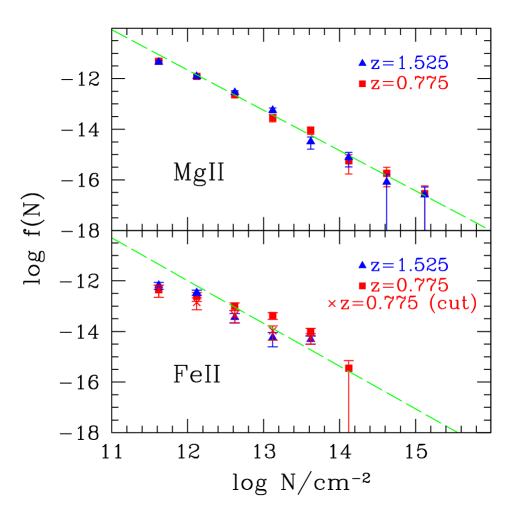
Figure 2: Column density distributions of Mg ii (upper panel) and Fe ii (lower panel) absorption components. In each panel, components are divided into two redshift bins: $0.4\leq z\leq 1.15$ (squares) and $1.15\leq z\leq 1.9$ (triangles). As in Fig. 1, the column density bins are $10^{0.5}N$ cm^-2 wide. The dashed lines correspond to the power-law fits described in the text, and in the lower panel we also include $f$ values when the large $z=0.836$ system in Q0002-422 is removed (see text).

In Figure 2 we plot $f(N)$ for both Mg ii and Fe ii, now going down to a minimum column density of $10^{11.5}$ cm^-2 which corresponds to roughly the same optical depth as $10^{12}$ cm^-2 for C iv and Si iv. For Mg ii and Fe ii the relevant doublets are at substantially longer restframe wavelengths, and therefore our UVES detections primarily occur at lower redshifts. Thus the mean redshifts of Mg ii and Fe ii are only 1.05, and 1.38, and we divide our data into bins from $0.4\leq z\leq 1.15$ and $1.15\leq z\leq 1.9.$ These lines arise in lower ionization gas and are often thought of as tracers of quiescent clouds, probably associated with galaxies (e.g. Petitjean & Bergeron 1990; Churchill et al. 1999; Churchill, Vogt, & Charlton 2003).

Like its higher-ionization counterparts, Mg ii is consistent with a lack of evolution in number densities over the observed redshift range. In the Fe ii case, however, a significant excess of intermediate column density components is found at lower redshifts. A closer inspection of the data indicates that this feature is caused by a single large system in Q0002-422, at $z=0.836$, which spans over 560 km s^-1. The removal of this system results in the third set of points in the lower panel of Fig. 2, which are consistent with the higher-redshift values. The large impact of this system in our measurements suggests that simple $\sqrt{N}$ estimates may somewhat underpredict the statistical error on our measurement. This hints at strong clustering between Fe ii components, which is in fact measured, as we discuss in detail below.

Statistical fluctuations aside, the overall density distributions of Mg ii and Fe ii are largely consistent with the power law fits obtained from previous measurements, apart from showing only a weak deviation in the lowest $N_{{\rm Fe\,\sc ii}}$ bin, probably due to incompleteness. In this case, the dashed-lined fits in Fig 2 are $f(N)=BN^{-\alpha}$ with $\alpha=1.6$ and $\log_{10}f=-13.2$ at $10^{13}$ cm^-2 for Mg ii and $\alpha=1.7$ and $\log_{10}f=-13.4$ at $10^{13}$ cm^-2 for Fe ii. While some flattening of $f_{{\rm Mg\,\sc ii}}(N)$ at even higher columns is necessary to match observations at column densities $\geq 10^{16.5}$ cm^-2 (Prochter, Prochaska, & Burles 2004), for the column densities in our sample our measured slopes are identical with those determined by previous studies. In particular our $\alpha$ fits match those of Churchill, Vogt, & Charlton (2003), although our $B$ values are different as these authors did not attempt to normalize their results by the total redshift path observed.

In summary, our automatic identification procedure produces a set of components whose column density distributions are consistent with previous measurements, complete to $N\lower 2.15277pt\hbox{$\;\buildrel>\over{\sim}\;$}10^{12}$ cm^-2 for C iv and Si iv, and complete to $N\lower 2.15277pt\hbox{$\;\buildrel>\over{\sim}\;$}10^{11.5}$ cm^-2 for Mg ii and Fe ii. No evolution in $f$ is seen for any species over the full redshift range probed, indicating that the majority of IGM enrichment is likely to have occurred before the redshifts observed in our sample.

Finally, our number densities allow us to compute the total cosmological densities of each of the detected species. Following S01, we express these in terms of a mass fraction relative to the critical density, which can be computed as

$$\Omega_{\rm ion}=\frac{H_{0}m_{\rm ion}}{c\rho_{\rm crit}}\frac{\sum N_{\rm ion}}{\Delta X}=1.4\times 10^{-23}A\frac{\sum N_{\rm ion}}{\Delta X},$$ (1)

where $H_{0}$ is the Hubble constant, $m_{\rm ion}$ is the mass of the given ion, $A$ is its atomic number, and $\Delta X$ is the total redshift path over which it is measured. The results of this analysis are given in Table 2. Note that these values are species densities, and no ionization corrections have been applied to estimate the corresponding element densities. Again these values are broadly consistent with previous measurements, although there is a significant scatter due to the fact that most of the material lies in the largest, rarest components. Thus previous studies have found $\Omega_{{\rm C\,\sc iv}}$ values as disparate as $6.8\times 10^{-8}$ at $z=2.5$ (S01), $3.8\pm 0.7\times 10^{-8}$ (BRS03), and between $3.5\times 10^{-8}$ and $7.9\times 10^{-8}$ depending on the method of analysis (Simcoe, Sargent, & Rauch 2004).

Species $\left<z\right>$ log(N/cm^-2) $\Omega$ $\Delta\Omega$ C iv 2.2 12-16 $7.54\times 10^{-8}$ $\pm 2.16\times 10^{-8}$ Si iv 2.4 12-16 $6.00\times 10^{-9}$ $\pm 1.21\times 10^{-9}$ Mg ii 1.1 11.5-16 $5.95\times 10^{-8}$ $\pm 2.23\times 10^{-8}$ Fe ii 1.4 11.5-16 $1.87\times 10^{-8}$ $\pm 0.36\times 10^{-8}$

Table 2: Cosmological densities of detected species.

4 Spatial Distribution

4.1 Carbon IV and Silicon IV

Having constructed a sample of well-identified metal absorption components, we then computed their two-point correlation function in redshift space, $\xi(v)$. This quantity was previously studied in Rauch et al. (1996) who noted a marked similarity between $\xi(v)$ of C iv and Mg ii, in BSR03, who carried out a two-Gaussian fit (see also Petitjean & Bergeron 1990, 1994), and in Paper I. For each quasar, we computed a histogram of all velocity separations and divided by the number expected for a random distribution. Formally, the correlation function for a QSO $\ell$ is

$$\xi^{\ell}(v_{k})+1=\frac{n^{\ell}_{k}}{\left<n^{\ell}_{k}\right>},$$ (2)

where $n^{\ell}_{k}$ is the number of pairs separated by a velocity difference corresponding to a bin $k$, and $\left<n^{\ell}_{k}\right>$ is the average number of such pairs that would be found in the redshift interval covered by QSO $\ell$, given a random distribution of redshifts with an overall density equal to the mean density in the sample. Alternatively, we may consider all QSOs at once and compute

$$\xi(v_{k})+1=\frac{\sum_{\ell}n^{\ell}_{k}}{\sum_{\ell}\left<n^{\ell}_{k}\right>},$$ (3)

or equivalently

$$\xi(v_{k})+1=\sum_{\ell}w^{\ell}_{k}\,[\xi^{\ell}(v_{k})+1]\quad{\rm with}\quad w^{\ell}_{k}\equiv\frac{\left<n^{\ell}_{k}\right>}{\sum_{\ell}\left<n^{\ell}_{k}\right>},$$ (4)

that is weighting the correlation found for each QSO by the number of random pairs that are expected given the redshift coverage of that QSO. The statistical variance in this measurement is given by

$$\sigma^{2}_{k}=\sum_{\ell}(w^{\ell}_{k})^{2}\sigma^{2,\ell}_{k},$$ (5)

where $\sigma^{2,\ell}_{k}$ is the variance associated with bin $k$ of quasar $\ell.$ In Paper I, we estimated this quantity according to the usual formula

$$\sigma^{2,\ell}_{k}=\frac{n^{\ell}_{k}}{\left<n^{\ell}_{k}\right>^{2}},$$ (6)

which gives the Poisson error in our measurement. In the results presented here, however, we adopt a more conservative approach, and also include the additional scatter caused by the finite sample size used to construct the correlation function (Mo, Jing, & Börner 1992). In this case

$$\sigma^{2,\ell}_{k}=\frac{1}{\left<n^{\ell}_{k}\right>^{2}}\left[n^{\ell}_{k}+4\frac{(n^{\ell}_{k})^{2}}{N^{\ell}}\right],$$ (7)

where $N^{\ell}$ is the total number of components detected in QSO $\ell$. Note that the presence of this additional scatter highlights the strength of our high signal-to-noise data set, as it allows us to work in the limit in which the number of C iv components detected in each quasar is large.

Figure 3: Two point correlation function of C iv (upper panel) and Si iv (lower panel) absorption components. In each panel the components have been divided into two redshifts bins, with symbols as in Fig. 1. The upper panel also includes a number of comparisons with previous measurements. In particular: the lower set of crosses corresponds to the full set of components defined in BSR03, normalizing each QSO individually; the upper set of crosses corresponds to imposing a column density cut of $10^{12}$ cm^-2, normalizing each QSO by its expected number of pairs; and the solid lines correspond to dividing the BSR03 data into a subsamples with $z\geq 3.1$ (lower line) and $z<3.1$ (upper line), as described in the text. In the lower panel, the crosses corresponds to imposing a column density cut of $10^{12}$ cm^-2 on the Si iv components observed in BSR03 and normalizing each QSO by its expected number of pairs.

The resulting correlation functions are shown in Fig. 3, again split into two redshift bins. Interestingly, in the better-measured C iv case, there are hints that the $z\leq 2.3$ correlation function may be enhanced with respect to the high-redshift one. Furthermore, this growth is consistent with a population of absorbers that “passively” evolves by following the motion of the IGM during the formation of structure, as we discuss in further detail in §8.

In the upper panel of this figure we also plot correlation functions computed from the sample defined in BSR03, which is drawn from the spectra of nine QSOs with a mean redshift of 3.1 and a signal-to-noise per pixel $\approx 50.$ In this case we show results obtained both from using the full data set, normalizing each quasar individually (as was carried out in BSR03), and from imposing a lower cut-off at $N_{{\rm C\,\sc iv},\rm min}=10^{12}$ cm${}^{-2},$ normalizing each quasar by the expected number of pairs (as was carried out in our analysis). In both cases the resulting $\xi_{{\rm C\,\sc iv}}$ values are similar and somewhat lower in amplitude than our measurements. Rauch et al. (1996) similarly have found a lower amplitude. Dividing the BSR03 data into a $z<3.1$ bin with a mean redshift of 2.5 and a $z>3.1$ bin with a mean redshift of 3.6 resulted in correlation functions given by the solid curves (again calculated according to our method). Furthermore the amplitude of the $z=2.5$ BSR03 correlation function is similar to our measurements, which are drawn from a sample with a mean redshift of $2.3.$ However, the higher-redshift curve is substantially lower, again indicating that $\xi_{{\rm C\,\sc iv}}$ is likely to evolve with redshift. This was also suggested by the analysis in BSR03 Figure 14, although they point out the changing ionizing background may also be an issue. Finally we note that while the BSR03 sample shows a relative lack of components at $\approx 500$ km/s. This is very near the C iv doublet separation.

Moving to the bottom panel, we see that the overall shape and amplitude of the C iv and Si iv correlation functions are similar and are consistent to within the Si iv measurement errors, as was discussed in Paper I. Both functions exhibit a steep decline at large separations and a flatter profile at small separations, with an elbow occurring at $\approx 150$ km s^-1. Both functions are also consistent with the correlation one obtains from the full BSR03 Si iv sample, after applying our cuts. Finally, as was noted in Paper I, there is a weak low redshift feature at $\approx 500$ km s^-1 in $\xi_{{\rm C\,\sc iv}}$, the origin of which we explore in §4.2.

Figure 4: Dependence of the C iv correlation function on column density threshold. Upper panel: Effect of applying a cut on the maximum column density of C iv components used to calculate $\xi_{{\rm C\,\sc iv}}(v)$. In all cases $N_{{\rm C\,\sc iv},\rm min}=10^{12}$ cm^-2. Lower panel: Effect of applying a cut on the minimum C iv column density, with $N_{{\rm C\,\sc iv},\rm max}$ fixed at 10¹⁶ cm${}^{-2}.$

In Fig. 4 we study the dependence of the C iv spatial distribution on column density, by computing the correlation function over the full redshift range but selecting components within a fixed range of column density. In the upper panel of this figure we apply a cut on the maximum column density component, while holding the minimum $N_{\rm C\,\sc iv}$ fixed at our detection limit of $10^{12}$ cm^-2. Apart from a weak shift in the 500-630 km s^-1 bin, $\xi_{{\rm C\,\sc iv}}(v)$ remains practically unchanged by this threshold. As the majority of the detected components are relatively weak, this indicates that our signal is determined by the bulk of the components in our sample, rather than by properties of individual strong absorbers.

The results of a more drastic test are shown in the lower panel of this figure. Here we hold $N_{{\rm C\,\sc iv},\rm max}$ fixed at $10^{16}$ cm^-2 and apply a cut on the minimum column density, which greatly reduces the number of components in the sample. Nevertheless moving from $N_{{\rm C\,\sc iv},\rm min}=10^{12}$ cm^-2 to $N_{{\rm C\,\sc iv},\rm min}=10^{13.5}$ cm^-2 results only in a very weak enhancement of $\xi_{{\rm C\,\sc iv}}(v)$ at small separations, while the rest of the correlation function remains unchanged. Thus, unlike Ly$\alpha$ absorption systems (Cristiani et al. 1997), the correlation of C iv does not depend strongly on absorption column densities. Instead, the spatial distribution seems to be a global property of the population of C iv components.

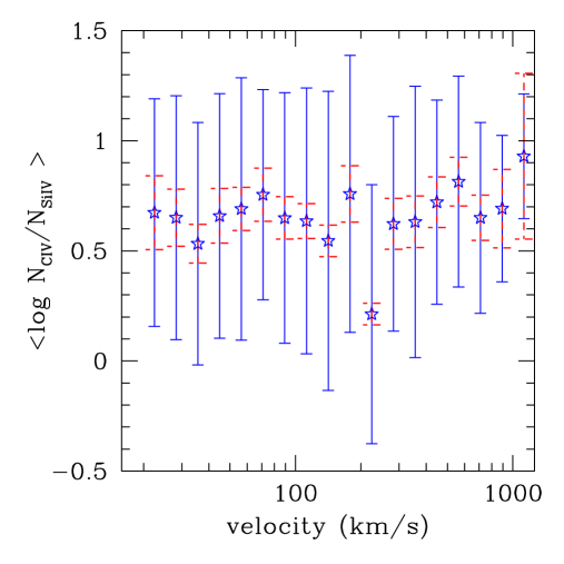
Figure 5: The average $\log(N_{\rm C\,\sc iv}/N_{\rm Si\,\sc iv})$ ratio for C iv components contributing to the correlation function at various separations. At each separation the dashed error bars are the statistical errors, while the solid error bars are the intrinsic scatter.

A question that immediately arises is whether the features observed in the C iv and Si iv correlation functions are intrinsic to the underlying distribution of metals, or perhaps arise from variations in the UV background at somewhat shorter wavelengths. In fact, analyses of the He ii distribution due to ionization by 54.4 eV photons suggest that the second reionization of hydrogen may still have been quite patchy at $z=2.3-2.9$ (Shull et al. 2004), with He ii found preferentially in “void” regions where HI is weak or undetected.

On the other hand, the ionization potentials of C iii and Si iii are 47.5 eV and 33.5 eV, respectively, somewhat lower than that of He ii, but well beyond the ionization potential of hydrogen. Thus if the suggested patchiness of He ii is due primarily to changes in the IGM opacity at wavelengths shortward of 54.4 eV, then the distribution of C iv and Si iv is likely to more closely trace the underlying distribution of metals. If He ii inhomogeneities exist and are caused by a sparsity of hard sources, however, it is possible that background variations may also play a role in the distribution of triply ionized regions of carbon and silicon.

As the ionization potentials of C iii and Si iii differ by 12 eV, each is sensitive to a slightly different range of UV photons. Thus if the features seen in Figure 3 were produced by changes in the ionizing background, one might expect to see systematic changes in the ratio of these species as a function of separation. As a simple test of this possibility, we considered the average $\log(N_{{\rm C\,\sc iv}}/N_{{\rm Si\,\sc iv}})$ as a function of separation. In order to make the sample included in this average as large as possible we computed this as

$$\left<\log(\frac{N_{{\rm C\,\sc iv}}}{N_{{\rm Si\,\sc iv}}})\right>_{k}\hskip-5.69046pt =\qquad\qquad\qquad\qquad\qquad\qquad\qquad\qquad\qquad$$ (8)

$$\sum_{i,j\in{\rm bin}_{k}}\sum_{\ell}\log\left(\frac{N_{{\rm C\,\sc iv},i}}{N_{{\rm Si\,\sc iv},l}}\right)\theta(5-|v_{\ell}-v_{i}|)$$

$$\hskip-8.5359pt\left\{\sum_{i,j\in{\rm bin}_{k}}\sum_{\ell}\Big{[}1\times\theta(5-|v_{\ell}-v_{i}|)\Big{]}\right\}^{-1},$$

where $\theta(v)$ is the Heaveside step function, $i$ and $j$ are indexes of C iv components, $l$ is an index over all Si iv components, and $k$ is a given bin in velocity separation used to calculate the correlation function. In other words, for each bin in the correlation function, we average $\log(N^{{\rm C\,\sc iv}}/N^{{\rm Si\,\sc iv}})$ over all C iv components $i$ that are found at the appropriate separation from another C iv component $j$ and within 5 km s^-1 of a Si iv component $l$.

The results of this analysis are found in Figure 5, which shows no correlation between separation and species abundances. Furthermore, our average value of $\log(N^{{\rm C\,\sc iv}}/N^{{\rm Si\,\sc iv}})\approx 0.7$ is similar to that seen in previous analyses of $10^{12}$ cm${}^{-2}\leq N_{{\rm C\,\sc iv}}\leq 3\times 10^{14}$ cm^-2 absorbers (Kim, Cristiani, & D’odorico 2002; BSR03), as well as the weaker C iv and Si iv lines detected by Aguirre et al. (2003) using the pixel optical depth method. Thus there is nothing particularly unusual about the subset of absorbers selected by our procedure. Although this is clearly not an exhaustive test, it nevertheless suggests that the features in the correlation functions are not imprinted in a straightforward way by the UV background itself, and are more likely to be caused by the spatial distribution of metals. However, a much more detailed analysis is necessary to settle this issue definitively.

4.2 Peculiar Systems at Low-Redshift

The C iv correlation functions in Figs. 3 and 4 hint at a secondary bump at large separations. It is important to try and understand if this comes from the presence of few peculiar systems or if this is a generic feature of the C iv distribution. To this end we computed the correlation function for different samples, each time excluding one of the lines of sight, and discovered that the signal comes from three QSOs, namely, PKS 0237$-$23, HE 0001$-$2340 and Q 0122$-$380.

Figure 6: Top: Impact of peculiar systems on the C iv correlation function. Here the square points are computed from the full sample, the circles are computed excluding the sightline towards PKS 0237$-$23, and the stars are computed excluding both PKS 0237$-$23 and the two sub-DLA systems, as described in the text. Bottom: Comparison between $\xi_{{\rm C\,\sc iv}}$ for the full sample, including associated absorbers (crosses), and excluding C iv components with 5000 km s^-1 of the quasar redshifts (squares).

The first of these has been long known to be very peculiar. Indeed, a huge C iv complex is seen toward PKS 0237$-$23 at eleven different redshifts over the range 1.596$-$1.676 (more than 10,000 km s^-1) with three main subcomplexes at $z_{\rm abs}$ = 1.596, 1.657 and 1.674 (Boroson et al. 1978, Sargent et al. 1988). Furthermore Folz et al. (1993) searched the field around PKS 0237$-$23 for other QSOs to provide background sources against which the presence of absorption at the same redshifts could be investigated. They concluded that the complex can be interpreted as a real spatial overdensity of absorbing clouds with a transverse size comparable to its extent along the line of sight, that is of the order of 30 Mpc. The correlation function without this line of sight is shown in Fig. 6.

Two other lines of sight display peculiar systems. At $z_{\rm abs}$ = 2.1851 toward HE 0001$-$2340 there is a sub-DLA system and the associated C iv system is spread over $\approx$450 km s^-1. It is therefore difficult to know if the structure there is due to large scales or more probably to the internal structure of the halo associated with this high density peak. At $z_{\rm abs}$ = 1.9743 toward Q 0122$-$380, there is a double strong system spread over more than 500 km s^-1. It is again difficult to know whether these absorptions reflect internal motions of highly disturbed gas.

After these are removed, the most significant excess at large separations is found in the 500-630 km s^-1 bin. This velocity difference corresponds to the difference in wavelengths of the C iv doublet itself. In fact, it is interesting to note that this bin is the only one that is significantly reduced by applying a cut to eliminate the larger $N_{{\rm C\,\sc iv}}$ components, as was seen in Fig. 4.

As a further test of large-separation correlations, we have also computed $\xi_{{\rm C\,\sc iv}}(v)$ including the associated systems, found within 5000 km s^-1 of the redshifts of the QSOs in this sample. This is compared with the C iv correlation function for our standard sample in the lower panel of Fig. 6. At all separations, $\xi_{{\rm C\,\sc iv}}$ remains unchanged, thus indicating that associated systems are not distributed in a particularly unusual way, and do not contribute any significant features to $\xi_{{\rm C\,\sc iv}}(v)$ at $\approx 500$ km s^-1, or any other separation.

4.3 Iron II and Magnesium II

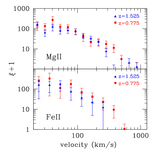
Figure 7: Upper panel: Two point correlation function of Mg ii, divided into two redshift bins as in Figure 2. Lower panel: Two point correlation function of Fe ii, divided into the same redshift bins.

We now turn our attention to the distribution of lower-redshift metals, as traced by Mg ii and Fe ii. Splitting the data into two redshift ranges yields the line-of-sight correlation functions shown in Fig. 7, where again we have included both the Poisson and sample-size errors in our estimate of the variances. Like their high-redshift counterparts, Mg ii and Fe ii are found to trace each other closely. Their correlation functions are both relatively shallow at small separations and fall off more steeply at large separations. Also like $\xi_{{\rm C\,\sc iv}}(v)$, both $\xi_{{\rm Mg\,\sc ii}}(v)$ and $\xi_{{\rm Fe\,\sc ii}}(v)$ exhibit slight enhancements at lower redshifts, although again these excesses fall within the errors.

Figure 8: Dependence of Mg ii correlation function on column density threshold. Upper panel: Effect of applying a cut on the maximum column density of Mg ii subcomponents used to calculate $\xi_{{\rm Mg\,\sc ii}}(v)$. In all cases $N_{{\rm Mg\,\sc ii},\rm min}=10^{11.5}$ cm^-2. Lower panel: Effect of applying a cut on the minimum Mg ii column density, with $N_{{\rm Mg\,\sc ii},\rm max}$ fixed at 10¹⁶ cm${}^{-2}.$

Next we examine the dependence of the Mg ii spatial distribution on column density. Removing the strongest absorbers in our sample before calculating $\xi_{{\rm Mg\,\sc ii}}(v)$ results in the values plotted in the upper panel of Figure 8. As in the C iv case, the Mg ii correlation function is not dominated by the clustering of large components, but rather remains almost unchanged as a function of $N_{\rm max}$, even when it is reduced to $10^{12.5}$ cm${}^{-2},$ excluding over a third of the systems. Similarly, raising the minimum column density from $10^{11.5}$ cm^-2 to $10^{12.5}$ cm^-2 does not boost $\xi_{{\rm Mg\,\sc ii}}(v)$, even though this excludes $\approx 2/3$ of the sample.

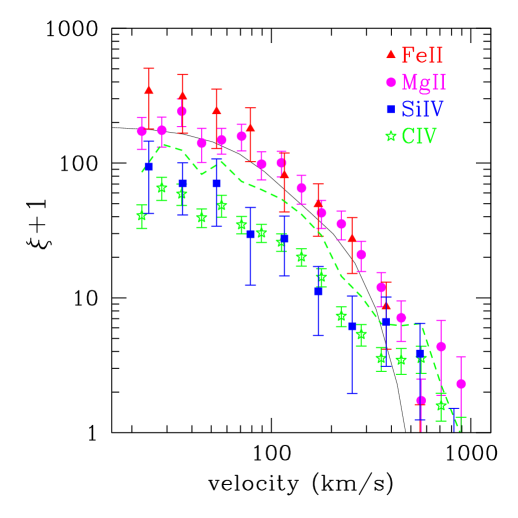
Figure 9: Measured correlation function of all metal-line components. Points are measurements from our sample, while the solid line is the Mg ii fit by Churchill, Vogt, & Charlton (2003), arbitrarily normalized. The dashed line is the C iv correlation function, shifted upwards by a factor of 2.1 to provide a simple estimate of the impact of structure formation from $z=2.2$ to 1.1 on a fixed population of absorbers.

In Figure 9 we compare the correlation functions of C iv and Si iv with those of Mg ii and Fe ii. Note that the mean redshift of these lower ionization species is $\approx 1.2$, while for C iv and Si iv $z_{\rm mean}\approx 2.3.$ Thus our sample contains very few objects in which all four species can be directly compared. Nevertheless, a comparison of their redshift-space correlation functions reveals a number of important parallels. While $\xi(v)$ of all species decline steeply at large separations and exhibit a turn-over at smaller velocity differences, the transition between these two regimes is pushed to slightly smaller separations in the Mg ii and Fe ii case, and the fall-off at higher densities is more abrupt.

Interestingly, the features seen in this distribution can be inferred from the original fitting to the distribution of velocity separations of Mg ii absorbers by Petitjean & Bergeron (1990), using a remarkably small number of systems. Their data were fit with the sum of two Gaussian distributions with similar overall weights and velocities dispersions of $\sigma_{v}=80$ km s^-1 and $\sigma_{v}=$ 390 km s^-1, which the authors interpreted as due to the kinematics of clouds bound within a given galaxy halo, and the kinematics of galaxies pairs, respectively. Working at higher spectral resolution and signal-to-noise, Churchill, Vogt, & Charlton (2003) also obtained a good two-component Gaussian fit to the two-point clustering function of Mg ii components, although they did not attempt to normalize this function to obtain $\xi_{\rm Mg\,\sc ii}(v)+1$. In this case the best-fit values were $\sigma_{v}=54$ km s^-1 and $\sigma_{v}=$ 166 km s^-1, where the relative amplitude of the narrow component was twice that of the broad component. This fit has been added to Figure 9, adopting an arbitrary normalization. Although our dataset has an overall signal-to-noise that is higher than that of Churchill, Vogt, & Charlton (2003), and thus is more complete at lower column densities, their two-Gaussian model also provide a good match to our data at $\Delta v\lower 2.15277pt\hbox{$\;\buildrel<\over{\sim}\;$}400$ km/s. However, it falls short of the observed correlation at larger separations.

To contrast the correlation functions in more detail, we have added a simple estimate of “passive” evolution to Figure 9, that is the evolution if the metals detected at $z\approx 2.3$ as C iv absorbers were to move along with the formation of structure before appearing as Mg ii absorbers at $z=1.2$. To first approximation, the overall bias of such a metal tracer field would remained fixed, but its correlation function would be enhanced by a factor of $D^{2}(1.2)$/$D^{2}(2.3)=2.1$, where $D(z)$ is the linear growth factor. Surprisingly, simply shifting $\xi_{{\rm C\,\sc iv}}$ by a factor of 2.3 provides us with an accurate match for the Mg ii correlation function over a large range of separations, although it underpredicts the clustering of Mg ii and Fe ii at smaller distances. This is dicussed in futher detail in §8.

To facilitate future comparisons, in Table 3 we give the correlation function and errors for each of the four species averaged over our full sample. Note that the small number of Si iv and Fe ii components forces us to use a smaller number of bins to beat down the statistical noise in our measurements.

bin (km s^-1) $\xi_{\rm C\,\sc iv}$ $\xi_{\rm Mg\,\sc ii}$ bin (km s^-1) $\xi_{\rm Si\,\sc iv}$ $\xi_{\rm Fe\,\sc ii}$ 20-25 41 $\pm$ 8 170 $\pm$ 50 20-30 94 $\pm$ 52 310 $\pm$ 150 25-32 66 $\pm$ 13 170 $\pm$ 40 30-43 71 $\pm$ 30 280 $\pm$ 130 32-40 59 $\pm$ 11 240 $\pm$ 60 43-65 71 $\pm$ 36 220 $\pm$ 100 40-50 40 $\pm$ 6 140 $\pm$ 40 65-100 30 $\pm$ 17 160 $\pm$ 70 50-63 49 $\pm$ 9 145 $\pm$ 30 100-140 27 $\pm$ 13 74 $\pm$ 34 63-79 35 $\pm$ 5 155 $\pm$ 40 140-200 11 $\pm$ 6 45 $\pm$ 19 79-100 30 $\pm$ 5 96 $\pm$ 23 200-300 6.2 $\pm$ 4.2 25 $\pm$ 11 100-125 26 $\pm$ 4 98 $\pm$ 21 300-450 6.6 $\pm$ 3.5 7.8 $\pm$ 4.1 125-160 20 $\pm$ 3 64 $\pm$ 15 450-670 3.9 $\pm$ 2.6 0.88 $\pm$ 0.58 160-200 14 $\pm$ 2 42 $\pm$ 10 670-1000 0.8 $\pm$ 0.7 0 $\pm$ 1 200-250 7.3 $\pm$ 1.2 35 $\pm$ 8 250-320 5.4 $\pm$ 1.0 20 $\pm$ 5 329-400 3.6 $\pm$ 0.7 12 $\pm$ 3 400-500 3.5 $\pm$ 0.7 6.9 $\pm$ 2.3 500-630 3.6 $\pm$ 0.8 1.7 $\pm$ 0.8 630-790 1.6 $\pm$ 0.4 4.2 $\pm$ 2.4 790-1000 0.98 $\pm$ 0.32 2.2 $\pm$ 1.3

Table 3: Summary of measured metal-component correlation functions. Note that there is likely to be significant redshift evolution of these functions. The mean redshifts of C iv and Si iv are $\approx 2.3$. The mean redshifts of Mg ii and Fe ii are $\approx 1.15.$

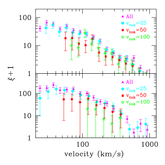
Figure 10: Upper panel: Impact of linking together C iv components into systems. Lower panel: Impact of linking together Mg ii components into systems. Details described in the text.

Finally, we carry out a test to determine if the spatial distribution of metals as traced by $\xi_{{\rm C\,\sc iv}}(v)$ may be affected by our VPFIT decomposition into components. Previous studies have attempted to trace the distribution of intergalactic metals by grouping together components into “systems,” which are likely to have a common physical origin, and computing the correlation function of these systems (e.g. Petitjean & Bergeron 1990; BSR03). While typically, system identifications have been carried out by eye, here we attempt a more objective approach, which parallels the friends-of-friends technique (Davis et al. 1985) widely used for group-finding in cosmological simulations. In this case, we define a velocity linking-length ($v_{\rm link}$) and group together all components whose separation from their nearest neighbor is less than $v_{\rm link}$ into a system at a redshift equal to the average over all its components. Note that this procedure does not involve simply linking together pairs within $v_{\rm link},$ but rather forms collections of many components, each within a linking length of its neighbors and grouped together into a single entity. It is therefore equivalent to partitioning a set of components into two systems whenever they are separated by a gap wider than $v_{\rm link}.$

In the upper panel of Figure 10 we plot $\xi_{{\rm C\,\sc iv}}(v)$ computed for the resulting C iv systems, for three different choices of $v_{\rm link}$. In all cases, within our measurement errors, combining components into systems has no appreciable impact at separations much larger than the linking length. Thus while BSR03 report a lack of clustering of systems as identified by eye, we are unable to reproduce this behavior with our automatic method. Perhaps this is not surprising, as the clustering of $\xi_{\rm C\,\sc iv}(v)$ is very strong, and thus many pairs of “systems” are likely to be closely spaced and easily tagged as a single object. However, our results show that fixing a pre-specified definition of systems does not remove large-scale correlations in this way.

In the lower panel of Figure 10, we see that grouping Mg ii components into systems has no clear impact at larger separations if $v_{\rm link}=25,$ $50$, and while there are hints of weak larger-scale damping if $v_{\rm link}=100$, these changes are within our errors. Similar results were obtained if each group was assigned the redshift of its largest component, leading us to conclude that the $\xi(v)$ features observed in both the high-redshift and low-redshift species are not related to division into components, but rather reflect the underlying distribution of intergalactic metals.

5 Numerical Simulation

5.1 Overall Properties

To better interpret the features seen in metal absorption-line systems, we conducted a detailed smoothed particle hydrodynamic (SPH) simulation of structure formation. Our goal here is to apply the same automated procedure used to identify metal absorbers in the LP data set to a detailed simulation, drawing conclusions as to what constraints our measurements place on the underlying distribution of IGM metals. For this purpose we focus our attention on a cold dark matter cosmological model with the same general cosmological parameters as above, and the additional parameters $\sigma_{8}=0.87$, and $n=1$, where $\sigma_{8}^{2}$ is the variance of linear fluctuations on the $8h^{-1}{\rm Mpc}$ scale, and $n$ is the “tilt” of the primordial power spectrum. The Bardeen et al. (1986) transfer function was used with an effective shape parameter of $\Gamma=0.2$, and the ionizing background flux was taken to be a Haardt & Madau (1996) spectrum with $J(\nu,z)=2.2\times 10^{-22}\,\left(\frac{\nu}{\nu_{\rm HI}}\right)^{-1}\,(1+z)^{0.73}\,\exp\left[-(z-2.3)^{2}/1.9\right]$ ergs s^-1 Hz^-1 cm^-2 sr^-1, corresponding to a photoionization rate of $6.8\times 10^{-13}\,(1+z)^{0.73}\,\exp\left[-(z-2.3)^{2}/1.9\right]$ s${}^{-1}.$

We simulated a box of size $40/h$ comoving Mpc on a side, using $320^{3}$ dark matter particles and an equal number of gas particles. The mass of each dark matter particle was $2.0\times 10^{8}\,{\rm M_{\odot}}$, and the mass of each gas particle was $3.4\times 10^{7}\,{\rm M_{\odot}}$. This yields a nominal minimum mass resolution for our (dark matter) group finding of $1.0\times 10^{10}\,{\rm M_{\odot}}.$ The run was started at an initial redshift of $z=99$, and a fixed physical S2 softening length of 6.7 kpc was chosen, which is equivalent to a Plummer softening length of 2.8 kpc. The simulation was conducted using a parallel MPI2-based version of the HYDRA code (Couchman et al. 1995) developed by the Virgo Consortium (Thacker et al. 2003).

We used the SPH algorithm described in Thacker et al. (2000), although in an improvement upon earlier work, the maximum SPH search radius now allows us to accurately resolve the mean density of the box. Photoionization was implemented using the publicly available routines from our serial HYDRA code. Radiative cooling was calculated using the Sutherland & Dopita (1993) collisional ionization equilibrium tables, and a uniform 2% solar metallicity was assumed for all gas particles for cooling purposes. Integration to $z=2.0$ required 9635 (unequal) steps, and four weeks of wall clock time on 64 processors. Outputs for post-processing were saved at redshifts of $z=8.0,$ 5.0, 4.0, 3.0, 2.5, and 2.0.

From each of the final three outputs, we interpolated to extract two-dimensional slices of overdensity, temperature, and line-of-sight peculiar velocities on 24 equally spaced planes. By extracting random sight-lines from each of these three fields, we were then able to generate simulated metal-line spectra, which could be processed in an identical fashion as the observed data. Before turning our attention to this issue, however, we first address the more basic concern of the overall hydrogen distribution, which serves as both a check of our simulation methods, and a way of fine-tuning the assumed ionizing background to reproduce the observed properties of the IGM.

5.2 Calculation of Neutral Hydrogen Fraction

Once the baryon density, temperature, and line-of sight velocity are extracted along a line of sight, constructing a simulated spectrum is relatively straightforward. One obtains the neutral hydrogen fraction, $f_{\rm HI}$, in the IGM by solving the ionization equilibrium equation (Black 1981)

$$\alpha(T)n_{p}n_{e}=\Gamma_{\rm ci}(T)n_{e}n_{\rm HI}+J_{22}G_{1}n_{\rm HI},$$ (9)

where $\alpha(T)$ is the radiative recombination rate, $\Gamma_{\rm ci}(T)$ is the rate of collisional ionization, $J_{22}$ is the UV background intensity in units of $10^{-22}$ ergs s^-1 Hz^-1 cm^-2 sr^-1, $J_{22}G_{1}$ is the rate of photoionization, and $n_{p},n_{e}$ and $n_{\rm HI}$ are the number densities of protons, electrons, and neutral hydrogen, respectively. For the Haardt & Madau (2001) spectrum assumed below $G_{1}=2.7\times 10^{-13}$ s^-1, for the original Haardt & Madau (1996) spectrum $G_{1}=3.2\times 10^{-13}$ s^-1, and for the $(\nu/\nu_{\rm HI})^{-1}$ spectrum used in our simulation $G_{1}=3.1\times 10^{-13}$ s^-1. For comparison, $G_{1}J_{22}$ is equal to $J_{-12}$ as defined in Choudhury et al. (2001) and $10G_{1}J_{21}$ as defined in Bi and Davidson (1997).

If we assume that the neutral fraction of hydrogen $\ll 1$ and all the helium present is in the fully-ionized form, we find

$$f_{\rm HI}(x,z)=\frac{\alpha\left[T(x,z)\right]}{\alpha\left[T(x,z)\right]+\Gamma_{\rm ci}\left[T(x,z)\right]+G1J_{22}n_{e}^{-1}(z)},$$ (10)

where the recombination rate $\Gamma_{\rm ci}(T)=5.85\times 10^{-11}T^{1/2}\exp(-157809.1/T)~{}{\rm cm}^{3}{\rm s}^{-1},$ with $T$ in Kelvin, and Black (1981) gives an approximate form for the recombination rate as

$$\frac{\alpha(T)}{{\rm cm}^{3}{\rm s}^{-1}}=\left\{\begin{array}[]{ll}4.36\times 10^{-10}T^{-0.7573}&\mbox{(if $T\geq 5000$K)}\\ 2.17\times 10^{-10}T^{-0.6756}&\mbox{(if $T<5000$K).}\end{array}\right.$$ (11)

With these expressions we can compute the neutral hydrogen density, $n_{\rm HI}[x,z(x)]$, along a line of sight. Here $x$ and $z$ are related by $c\,{\rm d}z={\rm d}x\,H(z)$, where the Hubble constant as a function of redshift is $H(z)=H_{0}\sqrt{\Omega_{\Lambda}+\Omega_{m}(1+z)^{3}}.$ We choose a coordinate system such that $x=0$ at the front of the box and define $\Delta z(x,z_{0})$ as the change in redshift from $x=0$. We then construct the Ly$\alpha$ optical depth as

$$\tau_{\alpha}(z_{0}+\Delta z)= \hskip-34.14322pt\displaystyle{\frac{c\sigma_{\alpha}}{(1+z_{0})\sqrt{\pi}}\int~{}{\rm d}x\frac{n_{\rm HI}(x,z_{0})}{b(x,z_{0})}}\times$$

$$\exp\left[-\left(\frac{xH(z_{0})+v(x,z_{0})(1+z_{0})-c\Delta z}{(1+z_{0})b(x,z_{0})}\right)^{2}\right],$$

where $b(x,z_{0})\equiv\sqrt{\frac{2k_{\rm B}T(x,z_{0})}{m_{p}}}$ (with $k_{B}$ the Boltzmann constant), $n_{H}(z)=1.12\times 10^{-5}(1-Y)\Omega_{b}(1+z)^{3}h^{2}\,{\rm cm}^{-3}=1.83\times 10^{-7}(1+z)^{3}\,{\rm cm}^{-3}$ (with $Y$ the helium mass fraction), and $\sigma_{\alpha}$ is the Ly$\alpha$ cross section, which can be calculated as

$$\sigma_{\alpha}=(3\pi\sigma_{T}/8)^{1/2}f\lambda_{0},$$ (13)

where $\lambda_{0}$ is the restframe wavelength of the transition, $f$ is the appropriate oscillator strength, and $\sigma_{T}=6.25\times 10^{-25}$ is the Thomson cross section. For Ly$\alpha$, $\lambda_{0}=1215$ Å  and $f=0.4162$, which gives $\sigma_{\alpha}=4.45\times 10^{-18}{\rm cm}.$ With eq. (5.2) in hand, we are able to construct simulated UVES spectra of the Lyman-$\alpha$ forest by stacking vectors of optical density computed from randomly extracted sightlines. These are then convolved with a Gaussian smoothing kernel with a width of 4.4 km s^-1 (corresponding to the UVES resolution) and rebinned onto a 205,000 array of wavelengths, using the UVES pixelization from 3,050 to 10,430 Å. Rather than interpolate between simulation outputs, however, we first turn our attention to a careful comparison between observations and limited segments of spectra at fixed redshifts, concentrating on two main quantities: the probability distribution function, a single-point quantity that is sensitive to the overall temperature and $J_{22}$ evolution background, and the two-point correlation function, a measure of the spatial distribution of the gas.

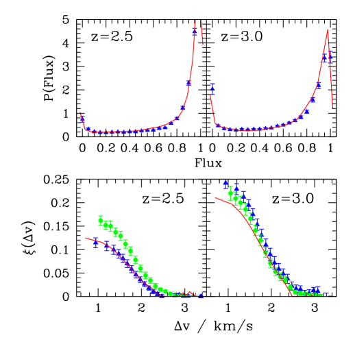
Figure 11: Top: Measured and simulated flux PDFs of the Lyman-$\alpha$ forest at two representative redshifts. Measurements are taken from McDonald et al. (2000) over redshift ranges of $2.09\leq z\leq 2.67$ (left panel) and $2.67\leq z\leq 3.39$ (right panel), respectively, while simulations are at fixed redshifts of 2.5 (left panel) and 3 (right panel). Bottom: Measured and simulated flux two-point correlation functions of the Lyman-$\alpha$ forest; $\xi(\Delta v)=<\delta F(v)\delta F(v+\Delta v)>$ where $\delta F=F/\bar{F}-1$, at two representative redshifts. The triangles are measurements by McDonald et al. (2000) over redshift ranges of $2.09\leq z\leq 2.67$ (left panel) and $2.67\leq z\leq 3.39$ (right panel) respectively and the circles are measurements by Croft et al. (2002) over redshift ranges of $2.31\leq z\leq 2.62$ (left panel) and $2.88\leq z\leq 3.25$ (right panel). Again the simulations, represented by the solid lines, are at fixed redshifts of 2.5 (left panel) and 3 (right panel).

5.3 Tests of The Numerical Hydrogen Distribution

The probability distribution (PDF) of the transmitted flux was first used to study the Ly$\alpha$ forest by Jenkins & Ostriker (1991) and since then has been a widely used tool for quantifying the mean properties of the IGM (e.g. Rauch et al. 1997, McDonald et al. 2000). In the upper panels of Figure 11 we compare the PDF as measured by McDonald et al. (2000) to that generated from 20 simulated spectra at representative redshifts of 2.5 and 3.0. In order to obtain the good agreement seen in this figure, it was necessary to adjust the assumed $J_{22}$ values to 4.7 at $z$ = 2.5 and 3.7 at $z$ = 3 (corresponding to photoionization rates of $1.3\times 10^{-12}$ s^-1 and $1.0\times 10^{-12}$ s^-1), down from the values of 5.4 and 4.7 (corresponding to photoionization rates of $1.7\times 10^{-12}$ s^-1 and $1.5\times 10^{-12}$ s^-1) respectively, that were assumed in the simulations.

This results in a slight inconsistency between the simulated $\rho$-$T$ relation and the one that would have arisen if we had repeated the simulation with our fit values of $J_{22}$. In practice however, this difference is unimportant in relation to our primary goal of constructing simulated metal lines. It is dwarfed by effects due to the uncertain evolution of the UV background at higher redshifts (e.g.  Hui & Gnedin 1997; Hui & Haiman 2003), uncertainties in the normalization of the quasar spectra (e.g. McDonald 2000) and the extrapolation of the UV background from 912Å  to the shorter wavelengths relevant for C iv and Si iv (e.g. Haardt & Madau 2001). Thus our approach is more than adequate for the purposes of this study. With our assumed background values, the mean fluxes at $z=2.5$ and $3.0$ are 0.794 and 0.692 respectively, while the observed values are $0.818\pm 0.012$ and $0.684\pm 0.023$.

As a second test of our simulations, we constructed the Lyman-$\alpha$ flux correlation function $\xi(\Delta v)=<\delta F(v)\delta F(v+\Delta v)>,$ which primarily provides a validation of our assumed primordial power spectrum $P(k)$ and its evolution in our simulation. Beginning with Croft et al. (1998), the direct inversion of the one dimensional power-spectrum of the Ly$\alpha$ flux has been seen as one of the best constraints on the shape of the mass power spectrum on intermediate scales (e.g. Hui 1999; McDonald et al. 2000; Pichon et al. 2001; Croft et al. 2002; Viel, Haehnelt, & Springel 2004).

Again, this quantity is straightforward to extract from our simulated spectra. The resulting values are shown in the lower panels of Figure 11, in which we compare them to measurements by McDonald et al. (2000) as well as Croft et al. (2002). As in the single-point case, our simulations are generally in good agreement with the observed values. In fact, at $z=2.5$, our simulated values are well within the range of values bracketed by the weakly disagreeing observational results. At $z=3.0$, our simulated values provide a slight underprediction at small separations, although this is only just outside the 1-$\sigma$ error in the current measurements. In summary then, the gas properties of our numerical simulation are more than adequate to provide a firm basis for the construction of Ly-$\alpha$ spectra, while at the same time containing sufficient resolution to allow us to push toward the denser regions associated with metal-line absorption systems.

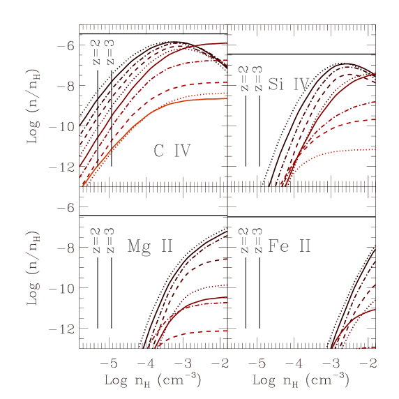
Figure 12: Abundances of various species as a function of total hydrogen number density for a $10^{-2}\,Z_{\odot}$ gas exposed to a Haardt & Madau (2001) background at $z=2.5$ In the upper left panel, the temperatures corresponding to each of the curves are, from top to bottom, $10^{3.75}$ K (dotted), $10^{4}$ K (solid), $10^{4.25}$ K (dot-dashed), $10^{4.5}$ K (dashed), $10^{4.75}$ K (dotted), $10^{5.0}$ K (solid), $10^{5.25}$ K (dot-dashed), $10^{5.5}$ K (dashed), $10^{5.75}$ K (dotted), and $10^{6.0}$K (solid). Similar labeling is used in the other panels. The vertical lines give the mean hydrogen number density at $z=3$ and 2 while the horizontal lines give the total abundance of each of the elements.

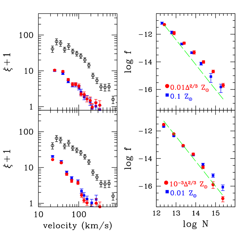
Figure 13: Correlation functions and column density distributions for models in which metallicity is assumed to be constant throughout the simulation, or a simple function of density. The filled points in the upper panels show high-metallicity models in which $Z=10^{-1}Z_{\odot}$ and $Z=\Delta^{2/3}10^{-2}Z_{\odot}$, while the filled points in the lower panels show lower metallicity models in which $Z=10^{-2}Z_{\odot}$ and $Z=\Delta^{2/3}10^{-3}Z_{\odot}.$ Fifty-seven simulated QSO sightlines were averaged in the high-metallicity models and 114 were averaged in the lower-metallicity cases. The open circles give the measured C iv correlation function, and the dashed lines give the fit to the column density distribution as in Figure 1.

6 Modeling Metal Enrichment

6.1 Calculation of Observed Metal Lines

Extending the methods of §5.2 to construct the spatial distribution of metal lines requires us to adopt an overall spectral shape for the ionizing background, as well as a more detailed calculation of the densities of various species. Here we assume a UV spectrum as predicted by the updated models of Haardt & Madau (2001; see also Haardt & Madau 1996) at $z=2.5$, but shifted such that $J_{22}$ is consistent with the levels found in $\S 5.$ Assuming local thermal equilibrium, we then make use of CLOUDY94 (Ferland et al. 1998; Ferland 2000) to construct tables of the relevant species as a function of temperature and density at each of these redshifts, for a characteristic metallicity of $10^{-2}{Z_{\odot}}$. Self-shielding in optically thick regions was not taken to account. The resulting species densities are shown as a function of hydrogen number density and temperature in Fig. 12, which is modeled after Figure 2 of Rauch, Haehenelt, & Steinmetz (1997).

In this figure, we see that, roughly speaking, C iv traces the widest range of environments, while Si iv, Mg ii, and Fe ii probe progressively denser regions. Thus while an appreciable level of C iv is found in only a few times overdense $z=3$ gas, comparable levels of Si iv are achieved only in denser regions with $\Delta\equiv\rho(x)/\bar{\rho}\approx 10$; and while Mg ii is found at similar densities to Si iv, Fe ii is only detectable in $\Delta\geq 100$ regions, orders of magnitude denser than most C iv regions.

Similarly, C iv is detectable over a large temperature range, covering from 10⁴ K up to $\approx 10^{6}$ K. While Si iv is also relatively stable with respect to temperature changes, Mg ii and Fe ii are much more fragile, and their abundances fall away quickly above $\approx 10^{5}$ K. From these results, we see that the correct modeling of Si iv requires simulations that probe to densities $\approx 10$ times higher than those most relevant to C iv, although $\xi_{{\rm C\,\sc iv}}(v)$ and $\xi_{{\rm Si\,\sc iv}}(v)$ trace each other closely. Thus while our numerical modeling was carried out at the highest resolution possible, we nevertheless limit our comparisons to C iv to minimize any remaining numerical effects.

6.2 A Nonlocal Dependence

Having determined the number densities of each of the species of interest as a function of temperature and density in a $10^{-2}{Z_{\odot}}$ medium, we then applied these calculations to extract simulated metal absorption spectra from our simulations. As a first step, following Rauch, Haehnelt, & Steinmetz (1997), we assumed a constant metallicity across the simulation volume and extracted sightlines of $\tau_{{\rm C\,\sc iv}}$ using an appropriately modified version of eq. (5.2):

$$\tau_{{\rm C\,\sc iv},i}(z_{0}+\Delta z)= \hskip-34.14322pt\displaystyle{\frac{c\sigma_{{\rm C\,\sc iv},i}}{(1+z_{0})\sqrt{\pi}}\int~{}{\rm d}x\frac{n_{{\rm C\,\sc iv}}(x,z_{0})}{b_{{\rm C\,\sc iv}}(x,z_{0})}\times}$$

$$\exp\left[-\left(\frac{xH(z_{0})+v(x,z_{0})(1+z_{0})-c\Delta z}{(1+z_{0})b_{{\rm C\,\sc iv}}(x,z_{0})}\right)^{2}\right],$$

where now $b_{{\rm C\,\sc iv}}(x,z_{0})_{\equiv}\sqrt{\frac{2k_{\rm B}T(x,z_{0})}{12m_{p}}},$ $n_{{\rm C\,\sc iv}}(z)$ is the mean C iv density, and $\sigma_{{\rm C\,\sc iv},i}$ is the cross section corresponding to the $i$th absorption line of the C iv doublet. These we compute directly from eq. (13) taking $(\lambda_{0,{\rm C\,\sc iv},1},\lambda_{0,{\rm C\,\sc iv},2})=(1548.2,1550.8)$ and $(f_{{\rm C\,\sc iv},1},f_{{\rm C\,\sc iv},2})=(0.1908,0.09522)$. For the low metallicities relevant for the IGM, the effects of changing metallicity can be modeled as a simple linear shift in the species under consideration.

In contrast with the fixed-redshift comparisons described in §5, our goal was to construct simulated data sets that corresponded as closely as possible to the full ESO Large Program data set. In this case, instead of stacking together spectra drawn from a single output, we instead allowed for redshift evolution: drawing slices from the output that most closely corresponded to the redshift in question, taking $n\propto(1+z)^{3}$, and interpolating between CLOUDY tables with appropriate $J_{22}$ values. Finally, we applied Poisson noise corresponding to a signal-to-noise of 100 per pixel.

Each spectrum generated by this method was subject to the same two-step identification procedure that was applied to the real data, and the resulting fits were subject to the same $N$ and $b$ cuts described in §2.2. The line lists compiled in this way were then used to generate correlation functions and column density distributions that directly parallel those calculated from the Large Program data set.

These are shown in Fig. 13, in which we explore a low-metallicity model ($10^{-2}Z_{\odot}$) roughly consistent with previous estimates (e.g. Rauch, Haehnelt, & Steinmetz 1997; Schaye et al. 2003) as well a higher-metallicity model ($10^{-1}Z_{\odot}$). Note that at these metallicities, changes in $Z$ can be modeled simply by boosting the C iv density derived from the CLOUDY tables by a linear factor. Increasing the metallicity by a factor of 10 in this way has very little effect on the correlation function: decreasing $\xi_{{\rm C\,\sc iv}}(v)$ in the 20 and 35 km s^-1 bins by roughly a factor of 1.5, while leaving the rest of the correlation function largely unchanged. In all cases these values fall far short of the clustering levels seen in our observational data, and they lack the conspicuous bend observed at $\approx 150$ km s^-1.

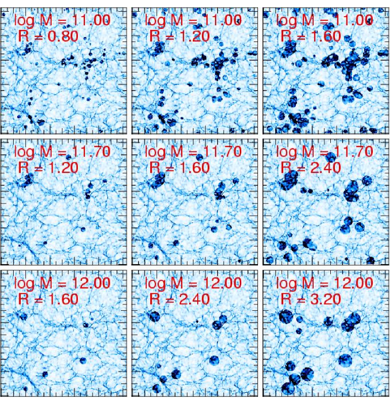
Figure 14: The C iv distribution of a $z=3$ slice in the simulation, dark regions are those contained within a distance $R_{s}$ from a dark matter halo of mass $M_{s}$, with parameters as labeled in the panels. These regions are used in constructing simulated spectra, while all gas outside them is considered to be metal-free. From left to right, and then top to bottom, the overall volume filling factors of these models are: 3.3%, 8.6%, 16.1%; 3.4%, 8.6%, 16.7%; and 1.7%, 5.5%, 11.6%

However, changing metallicity has a large effect on the column density distribution. The low-metallicity model is consistent with observations over the range of $12.5\leq\log N[{\rm cm}^{-2}]\leq 13.5$, and slightly overpredicts the number of large components (which have a negligible impact on the correlation function). The high-metallicity model, on the other hand, overpredicts the number of components for all column densities $\log N[{\rm cm}^{-2}]\geq 13.0.$

The poor fit to the correlation function is perhaps not surprising given the known inhomogeneity of the IGM metal distribution (e.g. Rauch, Haehnelt, & Steinmetz 1997). Most recently, this has been quantified by Schaye et al. (2003), who applied a pixel optical depth method to derive a nonlinear relation between the local overdensity $\Delta$ of hydrogen and the local carbon abundance. Over a large range of environments, they found $[C/H]\propto\Delta_{H}^{2/3}$ with a large variance. Is it possible that accounting for this relationship would be able to resolve the discrepancy in $\xi_{{\rm C\,\sc iv}}(v)$? In order to address this question, we repeated our experiment, assuming that the local density followed the best-fit relationship derived by Schaye et al. (2003). Again we considered both high and low metallicity models, resulting in correlation functions and column density distributions that are shown in Fig. 13.

As our results, which depend on a line-fitting procedure, are biased to the densest regions, the “zero point” metallicity of these models are naturally shifted to lower values. Thus, the $\Delta^{2/3}10^{-2}Z_{\odot}$ and the $\Delta^{2/3}10^{-3}Z_{\odot}$ models shown in these figures yield similar numbers of components as the single metallicity $10^{-1}Z_{\odot}$ and $10^{-2}Z_{\odot}$ models, respectively. In particular, the lower metallicity model allows us to obtain good agreement with the observed column density distribution, while assuming mean metallicity values more in line with previous estimates (e.g. Hellsten et al. 1997; Rauch, Haehenelt, & Steinmetz 1997; Schaye et al. 2003).

Introducing a $\Delta$ dependence has almost no effect, however, on the correlation function, neither boosting it at low separations nor introducing a feature at $\approx$ 150 km s^-1. Thus is appears that this nonlinear relationship is not the source of the clustering properties of the metal-line components, and rather that the large variance seen in the pixel-by-pixel results hides a third parameter that determines these features. In fact, in Paper I, we described just such a key parameter, the separation from a large dark-matter halo.

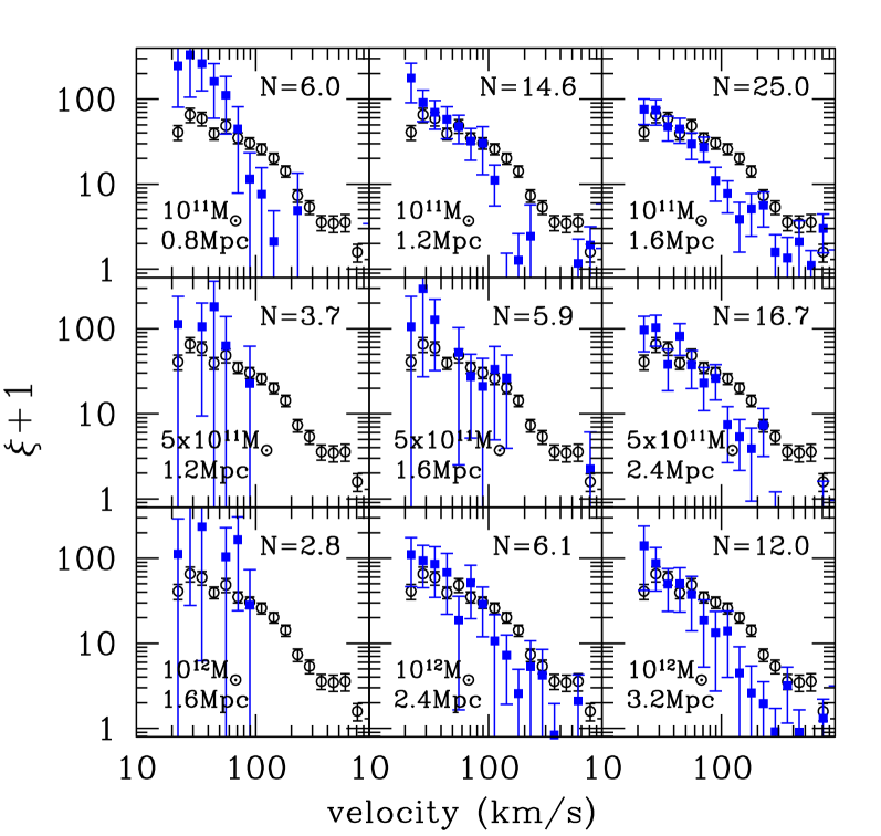
Figure 15: Correlation function of simulated C iv components, with an assumed bubble metallicity of $1/20Z_{\odot}$. Panels are labeled by their assumed $M_{s}$ in units of $\,{\rm M_{\odot}}$ and $R_{s}$ in units of comoving Mpc. In each panel the open circles summarize the observational results, while the filled circles represent the experimental results, as averaged over 114 spectra. Each panel is labeled by the average number of C iv components detected per simulated spectrum.

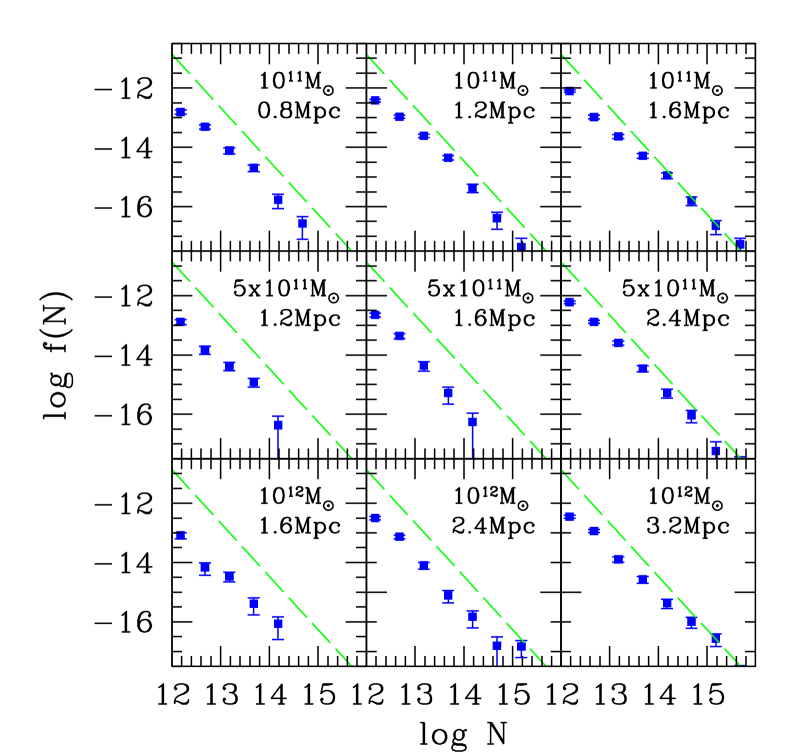
Figure 16: Column density distribution of simulated C iv absorption components, with an assumed bubble metallicity of $1/20Z_{\odot}$. Models are as in Fig. 16 and in each panel the filled points represent the simulation results, while the dashed line is the fit given in Figure 1.

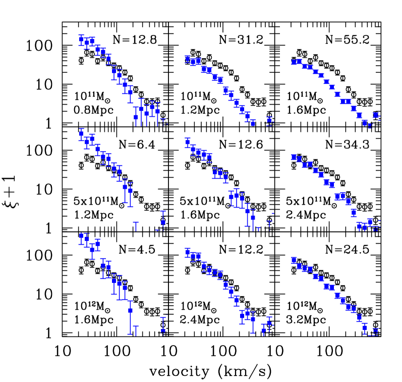
Figure 17: Correlation function of simulated C iv components, with an assumed bubble metallicity of $1/5Z_{\odot}$. Panels and symbols are as in Fig. 16.

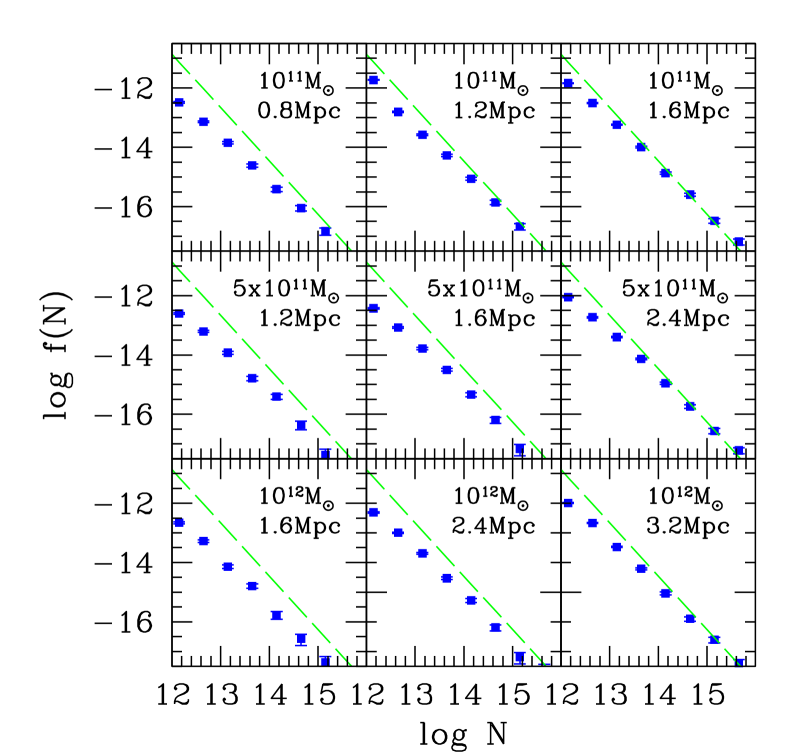
Figure 18: Column density distribution of simulated C iv absorption components, with an assumed bubble metallicity of $1/5Z_{\odot}$. Panels and symbols are as in Fig. 17.

7 Sources of Intergalactic Carbon IV

7.1 Distribution of Metals and Identification of Sources

While the observed features in the C iv correlation function can not be understood in terms of a local nonlinear relationship between the metal and density distributions, we saw in Paper I that these features could be easily explained in terms of the distribution of metal sources. In that work we used a pure dark-matter model to describe C iv components as contained within bubbles centered around sources, and we interpreted the amplitude and the knee in the C iv correlation function in terms of the source mass and bubble size, respectively. In this investigation we develop a similar model, but make use of the full gas and CLOUDY modeling described in §5 and §6.

Following Paper I, we adopt a parameterization in which all metals are found within a comoving radius $R_{s}$ of a dark matter halo whose mass is above a fixed value, $M_{s}$. To facilitate comparison with our previous modeling, as well as to allow for future comparisons with analytic approaches, we identified all sources at a fixed redshift of $z=3$. In particular, halo detection was performed using the HOP algorithm (Eisenstein & Hut 1998) with parameters $\delta_{\rm peak}=160$, $\delta_{\rm saddle}=140$, and $\delta_{\rm outer}=80$. The centres of these groups were then traced forward in time to the $z=2.5$ and 2.0 slices such that exactly the same groups could be selected from all the simulation slices, accounting for appropriate peculiar motions.

As in Paper I, our choice of $z=3$ is not meant to imply that enrichment occurred at this redshift, but rather that it occurred at an unknown redshift higher than the observed range, centered on groups whose large-scale clustering was equivalent to $z=3$ objects of mass $M_{s}$. For each choice of $R_{s}$ and $M_{s},$ we then painted bubbles of metals on our simulations, as illustrated in Fig. 14. While increasing $R_{s}$ has the obvious effect of increasing the volume filling factor of metals, increasing $M_{s}$ not only lowers this filling factor, but also clusters the bubbles more strongly. This can be most easily seen by comparing models with similar filling factors. For example, comparing the $M_{s}=1\times 10^{11}\,{\rm M_{\odot}},$ $R_{s}=1.6$ comoving Mpc slice to the $M_{s}=5\times 10^{11}\,{\rm M_{\odot}},$ $R_{s}=2.4$ comoving Mpc slice indicates that a similar fraction is enriched with metals in both cases, but these regions are spread over a considerable area in the lower-mass case and concentrated into dense knots in the higher-mass case.

7.2 Properties of Carbon-IV

From slices such as those shown in Fig. 14 we were able to generate simulated QSO absorption spectra, in a manner exactly parallel to that described in §6.2: drawing lines-of-sight for the various time outputs, piecing them together by evolving the mean density, interpolating between CLOUDY tables, and applying realistic levels of Poisson noise. In this case the metallicity was assumed to be at a fixed value $Z_{b}$ within each bubble, and zero everywhere else. Note, however, that our measurements are insensitive to C iv components with columns below $10^{12}$ cm^-2, a thus a more widely dispersed, lower-level contribution to IGM metals (e.g. Schaye et al. 2003; Bergeron & Herbert-Fort 2005) can not be excluded.

In Paper I, our modeling made use of a parameter $\tilde{b}$ that controlled the impact parameter associated with each sub-clump within a bubble. In our more physical modeling, this role is played by $Z_{b}$, which we fixed at an initial value of $1/20{Z_{\odot}}.$ These spectra were again analyzed by our automated procedure, and in Figures 15 and 16 we compare the resulting correlation functions and column density distributions with those measured in the Large-Programme data set.

These plots reflect the trends seen in the slices. Increasing the mass concentrates the metal into fewer regions, boosting the correlation function, particularly at large separations. Increasing $R_{s},$ on the other hand, impacts the correlation function primarily at smaller separations, and has a strong impact on the total number of C iv components detected per spectrum. From Fig. 15, the best-fit models are the $M_{s}=5\times 10^{11}\,{\rm M_{\odot}}$ & $R_{s}=2.4$ Mpc, $M_{s}=10^{12}\,{\rm M_{\odot}}$ & $R_{s}=2.4$ Mpc, and $M_{s}=10^{12}\,{\rm M_{\odot}}$ & $R_{s}=3.2$ Mpc cases, with filling factors of 5.5%, 8.6%, and 11.6% respectively although several of the lower filling-factor cases produce so few lines as to be difficult to evaluate in detail. Similar filling factors have been advocated by Pieri & Haehnelt (2005) on the basis of O vi measurements. The large $M_{s}$ values we derive are also suggestive of the regions around Lyman-Break galaxies (LBGs), which are observed to be clustered like $\approx 10^{11.5}\,{\rm M_{\odot}}$ halos at $z=3$ (Porciani & Giavalisco 2002), and for which a strong cross-correlation with C iv absorbers has been measured (Adelberger et al. 2003). It is also reminiscent of the association between galaxies and C iv absorbers put forward in BSR03.

In Fig. 16 we better quantify the number of components in each model, by constructing simulated column density distributions as discussed in §3.1. Here we see that regardless of our choice of source mass and bubble radius, all these models fall short of reproducing the observations. Due to the relatively small filling factors of such bubble models, our choice of $Z_{b}=1/20Z_{\odot}$ is not able to generate the relatively large number of C iv absorbers seen in the data.

In order to improve this agreement then, we considered a model in which we assume a higher bubble metallicity of $Z_{b}\approx 0.2Z_{\odot}$, generating the $\xi_{{\rm C\,\sc iv}}(v)$ and $\log f(N)$ values seen in Figures 17 and 18. As was the case for our $\tilde{b}$ parameter in Paper I, varying $Z_{b}$ has relatively little impact on the C iv correlation function, although the increased number of components does result in less noise.

Thus the high-metallicity simulations display the same trends and best-fit models as were seen in the lower $Z_{b}$ case, however the improved signal allows us to distinguish the $M_{s}=10^{12}\,{\rm M_{\odot}},$ $R=2.4$ Mpc model as a somewhat better match to the data than the $M_{s}=5\times 10^{11}\,{\rm M_{\odot}},$ $R=1.6$ Mpc and $M_{s}=10^{12}\,{\rm M_{\odot}},$ $R=3.2$ Mpc models. The improved signal in Fig. 17 also enables us to reject cases with very low filling factors. In particular, we see that the models with the smallest bubble sizes do not reproduce the observed $\approx 150$ km s^-1 elbow, exceeding the measured $\xi_{{\rm C\,\sc iv}}(v)$ at small separations. Furthermore, models with $M_{s}=10^{11}\,{\rm M_{\odot}}$ are now seen to fall far short of the observed correlation function at large separations, particularly if we consider the models with $R_{s}\geq 0.8$, which are not overly peaked at small distances.

Finally, assuming a mean bubble metallicity of $1/5Z_{\odot}$ has a large impact on the column density distribution, approximately doubling the number of detected components and bringing our best-fit model in rough agreement with the data, although perhaps even this value is slightly low in our best-fit cases. It is clear that we are forced toward these values because much of the gas around $\approx 10^{12}M_{\odot}$ is heated by infall above $\approx 10^{5.5}$ K, and thus it is largely in the outskirts of our bubbles in which C iv absorbers are found.

While, at face value, this metallicity is widely discrepant with other estimates, there are nevertheless two reasons to take it seriously. Firstly, the dense metal-rich regions in our model are observed to be enriched to similar levels at $z=1.2$. At this point, the LBG-scale halos around which we have placed our metals are expected to have fallen into clusters, and thus the IGM gas is detectable through X-ray emission in the intracluster medium (ICM). In fact, detailed Chandra and XMM-Newton observations indicate ICM iron levels of $Z=0.20^{+0.10}_{-0.05}$ at $z=1.2$ (Tozzi et al. 2003), implying that at even higher redshifts these metals have been efficiently mixed into the diffuse gas that forms into clusters. Secondly, we note that more than enough star formation has occurred by $z=2.3$ to enrich these regions to our assumed values. Indeed, comparisons between the integrated star formation history and more standard estimates of IGM metallicity have shown that a large fraction of $z\approx 2$ metals have so-far escaped detection (Pettini 1999). Thus, we find no compelling reason to dismiss this high metallicity value as spurious, although we emphasize that it has no direct impact on our derived clustering masses and bubble sizes.

8 An Analytic Model

While our simulated bubble model provides a compelling picture of the C iv and Si iv distribution at $z\approx 2-3$, it leaves open the question as to properties of Mg ii and Fe ii. Yet the detailed modeling of these species is beyond the capabilities of our simulation. As we saw in §6.1, the environments of Mg ii and Fe ii are denser than C iv and Si iv, particularly in the case of Fe ii. Even more constraining is the fact that almost all our detections of these systems fall well below our final simulated redshift of 2, with the majority lying in the $0.5\lower 2.15277pt\hbox{$\;\buildrel<\over{\sim}\;$}z\lower 2.15277pt\hbox{$\;\buildrel<\over{\sim}\;$}1.5$ redshift range.

In Fig. 9 we saw that while the overall shape and correlation function of these species is comparable to that observed in C iv and Si iv, the magnitude and long-separation tail of $\xi(v)$ are shifted upwards by a factor associated with the cosmological growth of structure. While reproducing these trends is beyond the capabilities of our simulation, they can nevertheless be studied from an approximate analytic perspective.

8.1 Derivation

In §7 we found good agreement between our observations and a model in which we painted metals around biased regions in our simulation. Analytically this corresponds to a picture in which the metal lines observed at $z_{\rm obs}$ come from clumps that are within a fixed radius of the sources of IGM metals. These pollution sources are associated with relatively rare objects of mass $M_{p}$ that ejected metals into surroundings at a high redshift $z_{p}>z_{\rm obs}$. After enrichment these components continue to cluster gravitationally to $z_{\rm obs}$.

In the numerical simulations, these pollution centres are identified with the galaxies of mass $M_{s}$ at a redshift of $z=3$. However, this mass and redshift were intended only to quantify the bias of sources, and it is more probable that they are really related to less massive, higher redshift objects, which exhibit similar clustering properties (Scannapieco 2005).

Let us consider then four points: the centres of two clumps (1 and 2), which we observe as metal-line components, and the centres of two bubbles (3 and 4), which correspond to the sources of pollution. We require that the pollution sources correspond to peaks [i.e. linear overdensities with a contrast larger than $\delta_{\rm cr}\equiv 1.68D(z_{p})^{-1}$] at a redshift $z_{p}>z_{\rm obs}$ and at a mass scale $M_{p}$. The clumps, on the other hand, are associated with the C iv absorbers themselves, and correspond to peaks at a mass scale $M_{c}$. In the linear approximation, these fields satisfy a joint Gaussian probability distribution which is specified by the block correlation matrix:

$${\mathbf{M}} = \left[\matrix{{{\xi}_{{\rm cc}}}(0)&\,{{\xi}_{{\rm cc}}}(r_{12})&\,{{\xi}_{{\rm cp}}}(r_{13})&\,{{\xi}_{{\rm cp}}}(r_{14})\cr\,{{\xi}_{{\rm cc}}}(r_{12})&{{\xi}_{{\rm cc}}}(0)&\,{{\xi}_{{\rm cp}}}(r_{23})&\,{{\xi}_{{\rm cp}}}(r_{24})\cr\,{{\xi}_{{\rm cp}}}(r_{13})&\,{{\xi}_{{\rm cp}}}(r_{23})&{{\xi}_{{\rm pp}}}(0)&\,{{\xi}_{{\rm pp}}}(r_{34})\cr\,{{\xi}_{{\rm cp}}}(r_{14})&\,{{\xi}_{{\rm cp}}}(r_{24})&\,{{\xi}_{{\rm pp}}}(r_{34})&{{\xi}_{{\rm pp}}}(0)\cr}\right]$$ (15)

$$\equiv \left[\matrix{{\mathbf{M}}_{\rm cc}&{\mathbf{c}}_{\rm cp}\cr{\mathbf{c}}_{\rm pc}&{\mathbf{M}}_{\rm pp}}\right]\,,$$

where $r_{ij}\equiv||{\mathbf{r}}_{i}-{\mathbf{r}}_{j}||$, and $\xi_{\rm pp}$, $\xi_{\rm cc}$ and $\xi_{\rm cp}$ refer respectively to the correlation between pollution centres, satellite clumps, and the cross correlation between clumps and the centres. The joint probability of having a peak of an amplitude larger than $\delta_{\rm cr}$ at the four points is given by

$$p(1,2,3,4) = \frac{1}{4\pi^{2}\sqrt{\det|{\mathbf{M}}|}}\int_{\delta_{\rm cr}}^{\infty}{{\mathrm{d}}{\delta}}_{1}\int_{\delta_{\rm cr}}^{\infty}{{\mathrm{d}}{\delta}}_{2}$$

$$\times \int_{\delta_{\rm cr}}^{\infty}{{\mathrm{d}}{\delta}}_{3}\int_{\delta_{\rm cr}}^{\infty}{{\mathrm{d}}{\delta}}_{4}$$

$$\times e^{-\frac{\left(\delta_{1},\delta_{2},\delta_{3},\delta_{4}\right)^{T}\cdot{\mathbf{M}}^{-1}\cdot\left(\delta_{1},\delta_{2},\delta_{3},\delta_{4}\right)}{2}}.\qquad$$

We will evaluate this expression, assuming that the threshold that defines the object is high relative to the corresponding rms densities and taking the correlation between the metal line clumps and the centres of pollution to be small. We shall not assume the smallness of the centre-centre nor clump-clump correlation, of which the first is the most important. In this limit

$${\mathbf{M}}^{-1} \approx \left[\matrix{{\mathbf{M}}^{-1}_{\rm cc}&-{\mathbf{M}}^{-1}_{\rm cc}{\mathbf{c}}_{\rm cp}{\mathbf{M}}^{-1}_{\rm pp}\cr-{\mathbf{M}}^{-1}_{\rm pp}{\mathbf{c}}_{\rm pc}{\mathbf{M}}^{-1}_{\rm cc}&{\mathbf{M}}^{-1}_{\rm pp}}\right]\,,$$ (17)

$$\det\left|{\mathbf{M}}\right| \approx \det\left|{\mathbf{M}}_{\rm cc}\right|\cdot\det\left|{\mathbf{M}}_{\rm pp}\right|,$$ (18)

and

$$p(1,2,3,4) \approx \frac{1}{4\pi^{2}\sqrt{\det|{\mathbf{M_{cc}}}|}\sqrt{\det|{\mathbf{M_{pp}}}|}}$$ (19)

$$\times \int_{\delta_{\rm cr}}^{\infty}{{\mathrm{d}}{\delta}}_{1}\int_{\delta_{\rm cr}}^{\infty}{{\mathrm{d}}{\delta}}_{2}e^{-\frac{1}{2}\left(\delta_{1},\delta_{2}\right)^{T}\cdot{\mathbf{M}}^{-1}_{\rm cc}\cdot\left(\delta_{1},\delta_{2}\right)}$$

$$\times \int_{\delta_{\rm cr}}^{\infty}{{\mathrm{d}}{\delta}}_{3}\int_{\delta_{\rm cr}}^{\infty}{{\mathrm{d}}{\delta}}_{4}e^{-\frac{1}{2}\left(\delta_{3},\delta_{4}\right)^{T}\cdot{\mathbf{M}}^{-1}_{\rm pp}\cdot\left(\delta_{3},\delta_{4}\right)}$$

$$\times e^{\left(\delta_{1},\delta_{2}\right)^{T}\cdot{\mathbf{M}}^{-1}_{\rm cc}{\mathbf{c}}_{\rm cp}{\mathbf{M}}^{-1}_{\rm pp}\cdot\left(\delta_{3},\delta_{4}\right)}.$$

In the high peak limit, the last cross-correlation term can be factored out from the integrals (see Appendix) yielding

$$p(1,2,3,4)\approx p(1,2)p(3,4)e^{\left(\delta_{cr},\delta_{cr}\right)^{T}\cdot{\mathbf{M}}^{-1}_{\rm cc}{\mathbf{c}}_{\rm cp}{\mathbf{M}}^{-1}_{\rm pp}\cdot\left(\delta_{cr},\delta_{cr}\right)},$$ (20)

where $p(1,2)$ and $p(3,4)$ are computed from eq. (36). Or, explicitly,

$$p(1,2,3,4) \approx \frac{1}{4\pi^{2}}\nu_{\rm cc}^{-2}\nu_{\rm pp}^{-2}{\rm C}\left[c(r_{12}),\nu_{\rm cc}\right]{\rm C}\left[c(r_{34}),\nu_{\rm pp}\right]$$

$$\times \exp\left[-\frac{\nu_{\rm cc}^{2}}{1+c_{\rm cc}(r_{12})}-\frac{\nu_{\rm pp}^{2}}{1+c_{\rm pp}(r_{34})}+\nu_{\rm cc}\nu_{\rm pp}\right.$$

$$\times \left.\frac{c_{{\rm cp}}(r_{13})+c_{{\rm cp}}(r_{24})+c_{{\rm cp}}(r_{14})+c_{{\rm cp}}(r_{23})}{\left[1+c_{{\rm pp}}(r_{34})\right]\left[1+c_{{\rm cc}}(r_{12})\right]}\right],$$

where the function ${\rm C}(x,\nu)$ is defined in the Appendix, and we define the cross-correlation coefficients as $c_{\rm cc}\equiv\xi_{\rm cc}(r)/\xi_{\rm cc}(0)$, $c_{\rm pp}\equiv\xi_{\rm pp}(r)/\xi_{\rm pp}(0)$, $c_{\rm cp}\equiv\xi_{\rm cp}(r)/\sqrt{\xi_{\rm cc}(0)\xi_{\rm pp}(0)}$, and the normalized density thresholds as $\nu_{\rm cc}\equiv\delta_{\rm cr}/\sqrt{\xi_{\rm cc}(0)}$ and $\nu_{\rm pp}\equiv\delta_{\rm cr}/\sqrt{\xi_{\rm pp}(0)}$.

Note that in eq. (8.1) the correlation functions in the denominator are not assumed to be small, which allows for proper accounting of the case when two clumps or two pollution centres are the same. For example, setting $r_{12}=r_{34}=0$ properly recovers the bivariant joint probability $p(1,3)$ to find a clump at a separation $r_{13}$ from the centre of pollution (equal in this case to $r_{14}=r_{23}=r_{24}$).

In our model only those clumps that lie within the spherical bubble around some pollution centre are observed to have metals. The correlation function of clumps of mass $M_{c}$ that are within spherical bubbles around peaks corresponding to the mass $M_{p}$, is defined as

$$p(\delta_{1},\delta_{3})p(\delta_{2},\delta_{4})\left[1+\bar{\xi}(r_{12})\right]\equiv\bar{p}(\delta_{1},\delta_{2},\delta_{3},\delta_{4}),$$ (22)

where the bar denotes averaging over position of pollution centres within a distance $R_{s}$ around two metal-rich clumps at a fixed separation $r_{12}$. Note that our definition of the correlation function, $\bar{\xi}(r_{12}),$ is not equivalent to the estimator of the underlying correlation function of all the clumps of mass $M_{c}$, $\xi(r_{12})$, nor is it equivalent to the conditional correlation function if there were a source of metals (a high peak of the scale $M_{p}$) in the vicinity of every small halo, $\bar{\xi}_{c}(r_{12})$, which would be given by

$$p(\delta_{1})p(\delta_{2})\bar{p}(\delta_{3},\delta_{4})\left[1+\bar{\xi}_{c}(r_{12})\right]\equiv\bar{p}(\delta_{1},\delta_{2},\delta_{3},\delta_{4}).$$ (23)

Furthermore, $\bar{\xi}(r_{12})$ depends on the underlying two-point correlation of small clumps, the correlation of the sources, and the cross-correlation between clumps and sources. This last term is subject to the most modification should the physics of metal dispersal change. However it mostly affects the biased density of small clumps in the vicinity of the sources relative to the cosmological mean, which is precisely the excess factored out in eq. (22).

Thus eq. (22) describes the correlation of metal components at the redshift of pollution, which is dominated by the clustering of the pollution sources. Subsequent gravitational clustering of enriched metals then leads to further amplification of the correlation in the linear approximation as

$$\bar{\xi}(r,z_{\rm obs})=\left[D(z_{\rm obs})/D(z_{p})\right]^{2}\bar{\xi}(r,z_{p}),$$ (24)

where $D(z)$ is the linear density growth factor. This growth is suggestive of the difference between the C iv and Mg ii correlation functions, as we saw in Fig 9, as well as the hints of evolution seen in $\xi_{{\rm C\,\sc iv}}(v)$ and $\xi_{{\rm Mg\,\sc ii}}(v)$ in Figs. 3 and 7.

8.2 Application to observed metal absorbers

Figure 19: Comparison of our analytic model with the data. Left panel: Low-redshift model for metal sources. Dotted lines represent the linear clustering at $z_{\rm obs}=2.3$ (lower) and $z_{\rm obs}=1.15$ (upper) of clumps observed in the vicinity of the pollution centres, with $M_{p}=10^{12}M_{\odot}$, $M_{c}=10^{9}M_{\odot}$ and $z_{p}=3$. Solid lines show the effect of applying a non-linear correction to these models. Finally, the dashed curve shows a nonlinear $z_{\rm obs}=1.15$ model in which $M_{p}=10^{12}M_{\odot}$, and $z_{p}=3,$ but now $M_{c}=10^{10}M_{\odot}.$ Right panel: Lower solid curve corresponds to $M_{p}=3\times 10^{9}M_{\odot}$, $M_{c}=10^{8}M_{\odot}$, $z_{\rm\rm pol}=7.5$, $z_{\rm obs}=2.3$, with no nonlinear correction applied. The upper solid line is a further linear extrapolation of this model to $z_{\rm obs}=1.15$. The upper dashed line is a linear model again with $z_{\rm obs}=1.15$ $M_{p}=3\times 10^{9}M_{\odot}$, $z_{\rm\rm pol}=7.5$, but with $M_{c}$ raised to $10^{9}M_{\odot}$. For all curves the comoving size of the bubble is $2.4$ Mpc.

In Figure 19 we fit our analytic model to the data. In the left panel we adopt the parameters used in our numerical simulations, identifying metal pollution centres with $M_{p}=10^{12}M_{\odot}$ objects at a redshift $z_{p}=3$ and metal rich clumps with collapsed objects of $M_{c}=10^{9}M_{\odot}$, with $R_{s}=2.4$ comoving Mpc. At $z_{\rm obs}=2.3,$ the analytic fit reproduces the measured $\xi_{{\rm C\,\sc iv}}(v)$ at large velocity separations, where it is dominated by the correlation between pollution centres, but it falls short at small velocities, where $\xi_{{\rm C\,\sc iv}}(v)$ is dominated by the clump distribution within each bubble.

This is because the smoothing imposed by choosing $M_{p}\approx 10^{12}M_{\odot}$ is similar to the 2.4 Mpc bubble size, and thus our linear formalism is insufficient to describe distances less than $R_{s}$. In reality, the nonlinear collapse of $M_{p}$ would have moved in new material to fill in this region. To mimic such nonlinear effects at small radii, we apply the prescription $\delta_{\rm cr}\to\delta_{\rm cr}+(1-1/\delta_{\rm cr})\xi$ (Mo & White 1996), resulting in the dashed curve. This correction, while crude, is seen to recover a $\xi_{{\rm C\,\sc iv}}(v)$ that is similar to our simulated $10^{12}M_{\odot}$, $R_{s}=2.4$ Mpc case (and thus the observed correlation function), confirming that the discrepancy at small distances is caused by our neglect of nonlinear motions.

Next we turn our attention to Mg ii and Fe ii, which are observed at lower redshifts $z\approx 1.2$. As we saw in Figure 9 the rise of the correlation amplitude of these species relative to C iv and Si iv is generally in agreement with the hypothesis of linear growth of gravitational clustering of a fixed population of objects from $z=2.3$ to $z=1.15$, although there are significant discrepancies at small radii. Again we plot both a linear $z_{\rm\rm pol}=3$, $M_{p}=10^{12}M_{\odot}$, $M_{c}=10^{9}M_{\odot}$ model observed at $z_{\rm obs}=1.15$ and a similar model in which a nonlinear correction has been applied. While the nonlinear curve does well at most radii, a shortfall is seen at $z\lower 2.15277pt\hbox{$\;\buildrel<\over{\sim}\;$}100$ km s^-1, similar to the discrepancy between the “shifted” $\xi_{{\rm C\,\sc iv}}(v)$ curve and the $\xi_{{\rm Mg\,\sc ii}}(v)$ curves in Figure 9. Based on our plots of the species fraction as a function of environment, an important difference between these species is clear. As Mg ii can only survive in regions with a low ionization parameter, it is biased toward much denser regions than C iv, which correspond in our analytic models to higher clump masses. Raising $M_{c}$ to $10^{10}M_{\odot}$ to account for this effect leads to the dashed curve in the left panel, which again agrees well with the data.

As discussed above, however, it is likely that the origin of metal pollution lies at higher redshift from sources of a lower mass, whose comoving clustering properties are identical to $M\approx 10^{12}M_{\odot}$ galaxies identified at $z=3$. Indeed, these biased high-redshift sources may be the progenitors that later grew into large $z=3$ galaxies. In the right panel of Figure 19 we explore such a high redshift model, in which we take $z_{\rm\rm pol}=7.5$ and $M_{p}=3\times 10^{9}M_{\odot}$, so that the bias of our sources is the same as for $M_{p}=10^{12}M_{\odot}$, objects forming at $z_{p}=3.$ Adopting a similar $\nu_{c}$ as in the $z_{p}=3$ case results in the solid curves. As the smoothing due to the Lagrangian radius associated with $M_{p}=3\times 10^{9}$ is minimal, no nonlinear correction is necessary and our simple model provides a reasonable fit to the C iv and Si iv components observed at $z=2.3.$

Similarly, extrapolation of the same objects to $z=1.15$, the mean redshift for Mg ii and Fe ii systems, matches their large scale ($v>300$ km s^-1) correlations quite well, although the data at these separations is sparse. At small velocities the difference between the environments of the two species becomes important, and linear scaling does not completely explain the enhancement of correlation amplitude in Fe ii and Mg ii relative to C iv and Si iv. As in the low redshift case, if we associate these species with larger clumps, the fit is much improved at small radii, resulting in the dashed curve.

In summary, our simple analytic model generally reproduces the features seen in our simulations of the C iv and Si iv correlation functions, although a nonlinear correction is necessary in the $z_{p}=3$ model. Linearly extrapolating these models to lower redshift results in a good fit to Mg ii and Fe ii at large distances, although a fit at smaller distances requires us to use larger clump masses, associated with denser environments. Finally, we find that there is a strong degeneracy between $M_{p}$ and $z_{\rm\rm pol},$ with a family of sources with similar biases producing acceptable fits.

9 Conclusions

While intergalactic metals are ubiquitous, the details of how these elements made their way into the most tenuous regions of space remains unknown. In this study we have used a uniquely large, homogeneous, and high signal-to noise sample of QSO sightlines to pin down the spatial distribution of these metals and combined this with advanced automated detection techniques and a high-resolution SPH simulation to pin down just what we can learn from this distribution. Our study has been focused on four key species: C iv and Si iv, which serve as tracers of somewhat-overdense regions from redshifts 1.5 to 3.0, and Mg ii and Fe ii, which trace dense, lower-redshift ($z=0.5-2.0$) environments. No evolution in the column density distributions of any of these species is detected.

In the high-redshift case, C iv and Si iv trace each other closely. For both species, $\xi(v),$ exhibits a steep decline at large separations, which is roughly consistent with the slope of the $\Lambda$CDM matter correlation function and the spatial clustering of $z\approx 3$ Lyman break galaxies. At separations below $\approx 150$ km s^-1, this function flattens out considerably, reaching a value of $\xi(v)\approx 50$, if $v\lower 2.15277pt\hbox{$\;\buildrel<\over{\sim}\;$}50$ km s^-1. Our data also suggests that $\xi_{\rm C\,\sc iv}(v)$ evolves weakly with redshift, at a level consistent with the linear growth of structure.

The distribution of metals as traced by $\xi_{\rm C\,\sc iv}(v)$ is extremely robust. We find that it remains almost completely unchanged when minimum or maximum column density cuts are applied to our sample, even if they are so extreme as to eliminate over two-thirds of the components. We have also linked together C iv components into systems, using a one-dimensional friends-of-friends algorithm, with linking lengths of $v_{\rm link}=$ 25, 50, and 100 km s^-1. In all cases, the line-of-sight correlation function of the resulting systems matches the original component correlation function (within measurements errors) at separations above $v_{\rm link}.$ Finally, the Si iv/C iv ratio shows no clear dependence when binned as a function of separation, suggesting that the features seen in $\xi_{\rm C\,\sc iv}(v)$ and $\xi_{\rm Si\,\sc iv}(v)$ do not result from fluctuations in the ionizing background.

Thus none of our tests indicate that the observed distributions of C iv and Si iv represent anything but the distribution of intergalactic metals at $z=1.5-3.0$. This motivated us to carry out a confrontation between our C iv observations and detailed simulations of IGM metal enrichment, which paralleled previous comparisons for the Lyman-alpha forest. Furthermore, the advanced automatic-detection procedures described in §2.2 (see also Aracil et al. 2005) allowed us not only to compare simulated and observed spectra, but generate simulated line lists in a manner that exactly paralleled the observations.

Using these tools, we found that the observed features of the C iv line-of-sight correlation function can not be reproduced if the IGM metallicity is constant. Rather any such model falls far short of the observed $\xi_{\rm C\,\sc iv}(v)$ amplitude and fails to reproduce flattening seen below $\approx 150$ km s${}^{-1}.$ Furthermore, adopting a local relation between overdensity and metallicity, as observed by Schaye et al. (2003), has little or no effect on these results.

On the other hand, rough agreement between simulated and observed C iv correlations is obtained in a model in which only a fraction of the IGM is enriched. Emulating the simple model in Paper I, we explored a range of models in which metals were confined within bubbles of radius $R_{s}$ about $z=3$ sources of mass $M_{s}$, where these quantities are not meant literally as source redshifts and masses, but rather as tracers of the bias of the $z_{\rm\rm pol}\geq 3$ source population. Varying these quantities, we derived parameters that suggest large metal bubbles, $R_{s}\approx 2$ comoving Mpc, around highly-biased sources, with $M_{s}\approx 10^{12}\,{\rm M_{\odot}}.$

These results are suggestive of the association between galaxies and C iv absorbers put forward in BSR03, and the high cross-correlation between LBGs and C iv absorbers measured by Adelberger et al. (2003). Yet this does not mean that LBGs are the sources of intergalactic metals, only that the $z_{\rm\rm pol}\geq 3$ sources were biased like LBGs. In fact, the case for outflows escaping lower-redshift starbursts is much more convincing than for dwarves (Martin 2005). Similarly, $R_{s}$ need not be interpreted as the ejection radius of each source, but instead as the distance at which bubbles from multiple sources overlap. Our best fit $M_{s}$ and $R_{s}$ values are independent of the assumed bubble metallicity, although the low $\lower 2.15277pt\hbox{$\;\buildrel<\over{\sim}\;$}10\%$ volume filling factors of these models forces us to use large $\approx 1/5Z_{\odot}$ values to reproduce the observed C iv column density distribution. Note however that given the high bias of our enriched regions, such metallicities may be necessary to reconcile $z\approx 2.3$ measurements with $z\approx 1.2$ observations of the iron content of the ICM in high-redshift galaxy clusters (Tozzi et al. 2003).

At lower redshifts, the line-of-sight correlation functions of Mg ii and Fe ii are consistent with the same enriched regions seen in C iv and Si iv, but now “passively” evolved down to $z\approx 1.2.$ Again both $\xi_{{\rm Mg\,\sc ii}}(v)$ and $\xi_{{\rm Fe\,\sc ii}}(v)$ trace each other closely, and exhibit the same steep decline at large separations and flattening at small separations as were seen in $\xi_{{\rm C\,\sc iv}}(v)$ and $\xi_{{\rm Si\,\sc iv}}(v).$ Also as in the higher redshift case, the Mg ii correlation function remains unchanged when minimum and maximum column density cuts are applied, and linking together Mg ii components into systems has no strong impact on $\xi_{{\rm Mg\,\sc ii}}(v)$ outside separations corresponding to the linking length.

Although Mg ii and Fe ii are detected in regions that can not be simulated numerically, we are nevertheless able to develop an analytic model that allows for a simple analysis of these species. Testing our model against $\xi_{{\rm C\,\sc iv}}(v)$ and $\xi_{{\rm Si\,\sc iv}}(v)$, we find generally good agreement with the data for similar values of mass and $R_{s}$ as in the numerical case. Pushing the model to lower redshift, we find that the same parameters do well at reproducing the clustering properties of Mg ii and Fe ii, especially when we account for the fact that the species are found in denser environments. Finally, we also find agreement with the observed $\xi_{{\rm C\,\sc iv}}(v)$ and $\xi_{{\rm Si\,\sc iv}}(v)$ at $z=2.3$ and $\xi_{{\rm Mg\,\sc ii}}(v)$ and $\xi_{{\rm Fe\,\sc ii}}(v)$ at $z=1.15$ and a high-redshift analytic model in which $z_{p}=7.5$ and $M_{p}=3\times 10^{9}\,{\rm M_{\odot}},$ illustrating the strong degeneracy between $M_{p}$ and $z_{p}$ for similarly biased sources.

Taken together, our $z\approx 2.3$ and $z\approx 1.2$ measurements, numerical simulations, and analytic modeling paint a consistent picture of IGM enrichment. The distribution of intergalactic metals does not appear uniform, nor simply dependent on the local density, but rather it bears the signature of the population from which it came. While the $z\geq 3$ redshift of metal ejection is unknown, a joint constraint on the masses and redshifts of the objects responsible for IGM pollution remains compelling. Models of IGM enrichment must come to terms with the observed biased sources of intergalactic metals.

Appendix A Two point joint probability distribution of high peaks in Gaussian fields

In this section we present formulas for the joint two point probability for the peaks in the Gaussian field that are used in our analytic model. These allow for the pair of peaks to have different scales and improve on the asymptotic results for the high peaks.

In the standard cosmological picture one identifies a collapsed object of mass $M$ with a peak of height $\delta>\delta_{cr}$ in the density field $\delta(x)$, smoothed with a top-hat window function $W(R)$ with the scale $R=\left(\frac{3M}{4\pi\bar{\rho}}\right)^{1/3}$. In the limit of large height the geometrical peaks of the Gaussian field can be approximately described as just the regions of high field values. This is the approximation that we adopt.

We shall need, first, the variance of the smoothed density field

$$\sigma^{2}=\int P(k)W^{2}(kR)k^{2}{{\mathrm{d}}{k}},$$ (25)

where $P(k)$ is the power spectrum of the density field and the Fourier image of the top-hat window is

$$W(kR)\equiv 4\pi R^{3}\left[\frac{\sin kR}{(KR)^{3}}-\frac{\cos kR}{(KR)^{2}}\right],$$ (26)

and, second, the correlation function between the values of the field at two positions, separated by the distance $r_{12}=x_{1}-x_{2}$

$$\xi(r_{12})=\int P(k)\frac{\sin(kr_{12})}{kr_{12}}W(kR_{1})W(kR_{2})k^{2}{{\mathrm{d}}{k}},$$ (27)

where the value at point $1$ is taken after the field is smoothed on a scale $R_{1}$ while at the point $2$ the field is evaluated after smoothing on a scale $R_{2}$. If $R_{1}=R_{2}$, then $\xi(0)=\sigma^{2}$, while in general $\xi(0)\leq\sigma_{1}\sigma_{2}$.

To evaluate the probability distribution functions used in §8 we begin with the well-known result for the one point probability of the field height to exceed $\delta_{cr}:$

$$p(1)=\frac{1}{\sqrt{2\pi}\sigma}\int_{\delta_{\rm cr}}^{\infty}{{\mathrm{d}}{\delta}}_{1}\exp\left[-\frac{\delta_{1}^{2}}{2\sigma_{1}^{2}}\right]\sim\frac{1}{\sqrt{2\pi}}\frac{\sigma_{1}}{\delta_{\rm cr}}\exp\left[-\frac{\delta_{\rm cr}^{2}}{2\sigma_{1}^{2}}\right]=\frac{1}{\sqrt{2\pi}}\nu_{1}^{-1}\exp\left[-\frac{\nu_{1}^{2}}{2}\right],$$ (28)

where $\nu_{1}\equiv\delta_{\rm cr}/\sigma_{1}.$ Here $1$ refers both to the (arbitrary) point where the field is evaluated, as well as to the scale it was smoothed with, $R_{1}$.

Next we evaluate the asymptotic behaviour at large $\delta_{\rm cr}\gg\sigma$ for the joint two-point probability

$$p(1,2)=\frac{1}{2\pi\sqrt{\sigma_{1}^{2}\sigma_{2}^{2}-\xi(r_{12})}}\int_{\delta_{\rm cr}}^{\infty}{{\mathrm{d}}{\delta}}_{1}\int_{\delta_{\rm cr}}^{\infty}{{\mathrm{d}}{\delta}}_{2}\exp\left[-\frac{1}{2}\frac{\delta_{1}\sigma_{2}^{2}+\delta_{2}\sigma_{1}^{2}-2\xi(r_{12})\delta_{1}\delta_{2}}{\sigma_{1}^{2}\sigma_{2}^{2}-\xi^{2}(r_{12})}\right]~{},$$ (29)

paying attention to the prefactors to the exponential terms. In general $\sigma_{1}\neq\sigma_{2},$ but when $\delta_{1}$ and $\delta_{2}$ represent the same field smoothed with the same filter taken at two different points (the case that we mostly need in this paper) $\sigma_{1}=\sigma_{2}$. Introducing uncorrelated variables $x=\frac{\delta_{1}\sigma_{2}+\delta_{2}\sigma_{1}}{\delta_{\rm cr}\sigma_{2}+\delta_{\rm cr}\sigma_{1}}$ and $y=\frac{\delta_{1}\sigma_{2}-\delta_{2}\sigma_{1}}{\sigma_{1}\sigma_{2}}$, we obtain

$$p(1,2)=\frac{\delta_{\rm cr}(\sigma_{1}+\sigma_{2})}{4\pi\sqrt{\sigma_{1}^{2}\sigma_{2}^{2}-\xi^{2}(r_{12})}}\int_{1}^{\infty}{{\mathrm{d}}{x}}\;\exp\left[-\frac{1}{4}\frac{\delta_{\rm cr}^{2}}{\sigma_{1}\sigma_{2}}\frac{(\sigma_{1}+\sigma_{2})^{2}}{\sigma_{1}\sigma_{2}+\xi(r_{12})}x^{2}\right]\int_{\frac{\delta_{\rm cr}[2\sigma_{2}-x(\sigma_{1}+\sigma_{2})]}{\sigma_{1}\sigma_{2}}}^{\frac{\delta_{\rm cr}[x(\sigma_{1}+\sigma_{2})-2\sigma_{1}]}{\sigma_{1}\sigma_{2}}}{{\mathrm{d}}{y}}\;\exp\left[-\frac{1}{4}\frac{\sigma_{1}\sigma_{2}}{\sigma_{1}\sigma_{2}-\xi(r_{12})}y^{2}\right].$$ (30)

This integral is of Laplace type $I=\int_{1}^{\infty}{{\mathrm{d}}{x}}\;e^{-\alpha\phi(x)}f(x)$, $\alpha=\frac{\delta_{\rm cr}^{2}}{\sigma_{1}\sigma_{2}}$ which for large $\alpha$ asymtotically accumulates at the lower integration boundary over the interval $x\in[1,1+\Delta x],~{}\Delta x=2\frac{\sigma_{1}\sigma_{2}}{\delta_{\rm cr}^{2}}\frac{\sigma_{1}\sigma_{2}+\xi(r_{12})}{(\sigma_{1}+\sigma_{2})^{2}}$. Asymtotic expansion is straightforward if one can expand $f(x)$ in the Taylor series near $x=1$

$$f(x)\equiv\int_{\frac{\delta_{\rm cr}[2\sigma_{2}-x(\sigma_{1}+\sigma_{2})]}{\sigma_{1}\sigma_{2}}}^{\frac{\delta_{\rm cr}[x(\sigma_{1}+\sigma_{2})-2\sigma_{1}]}{\sigma_{1}\sigma_{2}}}{{\mathrm{d}}{y}}\;e^{-\frac{1}{4}\frac{\sigma_{1}\sigma_{2}}{\sigma_{1}\sigma_{2}-\xi(r_{12})}y^{2}}\approx 2\left(x-1\right)\frac{\delta_{\rm cr}(\sigma_{1}+\sigma_{2})}{\sigma_{1}\sigma_{2}}\exp\left[-\frac{1}{4}\frac{\delta_{\rm cr}^{2}}{\sigma_{1}\sigma_{2}}\frac{(\sigma_{1}-\sigma_{2})^{2}}{\sigma_{1}\sigma_{2}-\xi(r_{12})}\right],$$ (31)

in which case we get

$$p(1,2)\approx\frac{2}{\pi}\frac{\sigma_{1}\sigma_{2}}{\delta_{\rm cr}^{2}}\frac{[\sigma_{1}\sigma_{2}+\xi(r_{12})]^{3/2}}{(\sigma_{1}+\sigma_{2})^{2}(\sigma_{1}\sigma_{2}-\xi(r_{12}))^{1/2}}\exp\left[-\frac{1}{2}\delta_{\rm cr}^{2}\frac{\sigma_{1}^{2}+\sigma_{2}^{2}-2\xi(r_{12})}{\sigma_{1}^{2}\sigma_{2}^{2}-\xi^{2}(r_{12})}\right].$$ (32)

Two things are notable. First is the prefactor $(\sigma_{1}\sigma_{2})/\delta_{\rm cr}^{2}$. Second, we find that for small correlations the effect in the exponent where small $\xi/\sigma_{1}\sigma_{2}$ is multiplied by $\delta_{\rm cr}/\sigma_{1}\sigma_{2}$ dominates the correction from the prefactor. Thus, as a leading order approximation, we can account for small correlations by factoring out the exponential correlation term from the original expression, with the values of the field replaced by the threshold values.

In reality, the asymptotics in eq. (32) do not give an accurate approximation if correlations are strong $\xi(r_{12})\to\sigma_{1}\sigma_{2}$, especially since our threshold parameter $\delta_{\rm cr}/\sigma$ may not be very large. This is definitely the case for a distribution of identical objects at short distances, since then $\xi(r\to 0)=\sigma^{2}$. More accurately, the Taylor expansion of $f(x)$ in eq.(31) is not suitable when the width of the relevant integration range $\Delta y=\delta_{\rm cr}\Delta x(\sigma_{1}+\sigma_{2})/(\sigma_{1}\sigma_{2})$ exceeds the width of the Gaussian $\sqrt{\left[\sigma_{1}\sigma_{2}-\xi(r_{12})\right]/(\sigma_{1}\sigma_{2})}$. In this case, however, the integration over $y$ can be extended to $\pm\infty.$ With subsequent asymptotic analysis of the integral over $x$ this gives

$$p(1,2)\approx\frac{1}{\sqrt{\pi}}\frac{\sqrt{\sigma_{1}\sigma_{2}}}{\delta_{\rm cr}}\frac{\sqrt{\sigma_{1}\sigma_{2}+\xi(r_{12})}}{\sigma_{1}+\sigma_{2}}\exp\left[-\frac{1}{4}\frac{\delta_{\rm cr}^{2}}{\sigma_{1}\sigma_{2}}\frac{(\sigma_{1}+\sigma_{2})^{2}}{\sigma_{1}\sigma_{2}+\xi(r_{12})}\right],~{}~{}~{}~{}\frac{2}{\sqrt{\sigma_{1}\sigma_{2}-\xi(r_{12})}}\frac{\sigma_{1}\sigma_{2}+\xi(r_{12})}{\sigma_{1}+\sigma_{2}}\gg\frac{\delta_{\rm cr}}{\sqrt{\sigma_{1}\sigma_{2}}}\gg 1$$ (33)

The general eqs. (32)-(33) are much simpler in the case when variances are identical $\sigma_{1}^{2}=\sigma_{2}^{2}=\xi(0)$. Defining the cross correlation coefficient $c(r_{12})=\xi(r_{12})/\xi(0)$ and specifying accurately the range of validity of eq. (32) gives

$$p(1,2) \approx \frac{1}{2\pi}\nu^{-2}\;{\rm A}\left[c(r_{12})\right]\exp\left[-\frac{\nu^{2}}{1+c(r_{12})}\right]~{}~{}~{},~{}~{}~{}~{}\nu\gg\max\left(1,\frac{1+c(r_{12})}{\sqrt{1-c(r_{12})}}\right),$$ (34)

$$p(1,2) \approx \frac{1}{\sqrt{2\pi}}\nu^{-1}\;{\rm B}\left[c(r_{12})\right]\exp\left[-\frac{\nu^{2}}{1+c(r_{12})}\right]~{},~{}~{}~{}~{}\frac{1+c(r_{12})}{\sqrt{1-c(r_{12})}}\gg\nu\gg 1~{}~{},$$ (35)

where smooth functions $A(x)\equiv\sqrt{\frac{(1+x)^{3}}{1-x}}\stackrel{{\scriptstyle x\to 0}}{{\longrightarrow}}1$ and $B(x)\equiv\sqrt{\frac{1+x}{2}}\stackrel{{\scriptstyle x\to 1}}{{\longrightarrow}}1$. As expected, $p(1,2)\stackrel{{\scriptstyle c\to 0}}{{\longrightarrow}}p(1)p(2)$ and $p(1,2)\stackrel{{\scriptstyle c\to 1}}{{\longrightarrow}}p(1)$. It is important to note that the probability is additionally enhanced by $\nu=\delta_{\rm cr}/\sigma$ when correlations are strong.

Finally, we combine equations (34)-(35) into the uniform approximation

$$p(1,2)\approx\frac{1}{2\pi}\nu^{-2}\;{\rm C}\left[c(r_{12}),\nu\right]\exp\left[-\frac{\nu^{2}}{1+c(r_{12})}\right]~{},~{}~{}~{}~{}\nu\gg 1,$$ (36)

with the help of an interpolating function, ${\rm C}(x,\nu)$, such that ${\rm C}(0,\nu)=1,~{}{\rm C}(1,\nu)=\nu\sqrt{2\pi}$. The choice

$${\rm C}(x,\nu)=\frac{\nu\sqrt{\pi}\sqrt{(1+x)^{3}}}{\left(\nu\sqrt{\pi}-1\right)\sqrt{1-x}+(1+x)}$$ (37)

reflects both the details of the functions $A(x)$ and $B(x)$ and of the transition between equations (34)-(35).

In the weak correlation regime, the formula (36) coincides with the classic result of Kaiser (1984). At the same time in the strong correlation regime, the result (36) shows that the correlation between regions of high density is additionally enhanced by $\sqrt{2\pi}\nu$ factor. Although our result is rigorous for the points of high excursions of the field at all separations $r$, the interpretation of the last regime in terms of peak, or object, correlation, is questionable at $r<R_{1}+R_{2}$ when the two high-density points likely belong to the same peak.

References

- [1] Adelberger, K. L., Steidel, C. C., Shapley, A. E., & Pettini, M. 2003, 584, 45
- [2] Aguirre, A., Schaye, J., Kim, T.-S., Theuns, T., Rauch, M., & Sargent, W. L. W. 2004, ApJ, 602, 38
- [3] Aracil, B. Petitjean, P., Pichon, C., & Bergeron, J. 2004, A&A, 419, 811
- [4] Aracil, B. et al. , in preparation, 2005
- [5] Bardeen, J. M., Bond, J. R., Kaiser, N., & Szalay, A. 1986, ApJ, 304, 15
- [6] Bergeron, J., Aracil, B., Petitjean, P., & Pichon, C. 2002, A&A, 396, L11
- [7] Begelman, M. C, Blandford, R. D. & Rees, M. J. 1984, Rev. Mod. Phys. 56, 255
- [8] Bergeron, J., & Herbert-Fort, S., IAU 199 Conference Proceedings, (astro-ph/0506700)
- [9] Bi H., Davidsen A. F., 1997, ApJ 479, 523
- [10] Black J. H., 1981, MNRAS, 197, 553
- [11] Boksenberg, A., Sargent, W. L. W., & Rauch, M. 2003, ApJS, submitted (astro-ph/0307557; BSR03)
- [12] Boroson, T., et al. , 1978, ApJ 220, 772
- [13] Bromm V., Ferrara A., Coppi P. S., & Larson R. B. 2001, MNRAS, 328, 969
- [14] Bromm, V., Yoshida, N., & Hernquist, L. 2003, ApJ, 596, L135
- [15] Carswell, R. F., Webb, J. K., Baldwin, J. A., & Atwood, B. 1987, ApJ, 319, 709
- [16] Carswell, R. F., Schaye, J., & Kim, T. S. 2002, ApJ, 578, 43
- [17] Cen, R., & Bryan, G. 2001, ApJ, 546, 81
- [18] Choudhury, T. R., Srianand, R., & Padmanabhan, T., 2001, ApJ, 559, 29.
- [19] Churchill, C. W., Rigby, J. R., Charlton, J. C., & Vogt, S. S. 1999, ApJS, 120, 51
- [20] Churchill, C. W., Vogt, S. S., & Charlton, J. C. 2003, AJ, 125, 98
- [21] Cristiani, S., D’Odorico, S., D’Odorico V., Fontana, A., Giallongo, E., & Savaglio, S., 1997, MNRAS, 285 209
- [22] Croft, R. A. C.. Weinberg, D. H., Katz, N. & Herquist, L., 1998, ApJ, 495, 44
- [23] Croft, R. A. C., et al. 2002, ApJ 581, 20
- [24] Couchman, H. M. P., Thomas, P. A., & Pearce, F. R. 1995, ApJ, 452, 797
- [25] Davis, M., Efstathiou, G., Frenk, C. S., & White, S. D. M. 1985, ApJ, 292, 371
- [26] Eisenstein, D. J. & Hut, P. 1998, ApJ, 498, 137
- [27] Eke, V. R., Cole, S., & Frenk C. S. 1996, MNRAS, 282, 263
- [28] Ellison, S. L., Songaila, A., Schaye, J., & Pettini, M. 2000, AJ, 120, 1175
- [29] Fan, X. et al. 2001, AJ, 121, 54
- [30] Ferland, G. J. 2000, MxAC, 9, 153
- [31] Ferland, G. J., Korista, K. T., Verner, D. A., Ferguson, J. W., Kingdon, J. B., & Verner, E. M. 1998, PASP, 100, 761
- [32] Frye, B., Broadhurst, T., & Benitez, N., 2002, ApJ, 568, 558
- [33] Foltz, C. B.,et al., 1993, AJ 105, 22
- [34] Gnedin, N. Y. & Ostriker J. P. 1997, ApJ, 486, 581
- [35] Haardt, F. & Madau, P. 1996, ApJ, 461, 20
- [36] Haardt, F. & Madau, P. 2001, in Proc. XXXVI Rencontres de Moriond (astro-ph/0106018)
- [37] Heisler, J., Hogan, C. J., & White, S. D. M. 1989, ApJ, 347, 52
- [38] Hellsten, U., Davé, R., Hernquist, L., Weinberg, D. & Katz, N. 1997, ApJ, 487, 482
- [39] Hui, L., & Gnedin, N. 1997, ApJ, 586, 581
- [40] Hui, L. 1999, ApJ, 516, 519
- [41] Hui, L., & Haiman, Z. 2003, ApJ, 596, 9
- [42] Jenkins, E. B. & Ostriker, J. P. 1991, ApJ, 376, 33
- [43] Jing, Y. P. 1999, ApJ, 515, L45
- [44] Kaiser, N. 1984, ApJ, 284, L9
- [45] Kim, T.-S., Cristiani, S. & D’Odorico 2002, A&A, 383, 747
- [46] Madau, P., Ferrara, A., & Rees, M. J. 2001, ApJ, 555, 9
- [47] Martin, C. L. 2005, ApJ, 621, 227
- [48] McDonald, P., Miralda-Escudé, J., Rauch M., Sargent, W. L. W., Barlow, T. A., Cen R., & Ostriker, J. P. 2000, ApJ, 543, 1
- [49] Mo, H. J., Jing, Y. P., & Börner, G. 1992, ApJ, 392, 452
- [50] Mo, H. J., & White, S. D. M. 1996, ApJ, MNRAS, 282, 348
- [51] Norman, M., O’Shea, B., & Paschos, P. 2004, ApJ, 601, L115
- [52] Perlmutter, S. et al. 1999, ApJ, 517, 565
- [53] Petitjean, P. & Bergeron, J. 1990, A&A, 231, 309
- [54] Petitjean, P. & Bergeron, J. 1994, A&A, 283, 759
- [55] Petitjean, P. 2001, ApSS 277, 517
- [56] Pettini, M. 1999, in Chemical Evolution from Zero to High Redshift, Proc. ESO Workshop, ed. J. Walsh & M. Rosa (Berling: Springer), 233
- [57] Pettini, M. et al., 2001, ApJ, 554, 981
- [58] Pettini, M., Madau, P., Bolte, M., Prochaska, J. X., Ellison, S., & Fan, X. 2003, ApJ , 594, 695
- [59] Pichon, C., Vergely, J. L., Rollinde, E., Colombi, S., & Petitjean, P. 2001, MNRAS, 326, 597
- [60] Pichon, C., Scannapieco, E., Aracil, B., Petitjean, P. Aubert, D., Bergeron, J., & Colombi S. 2003, ApJ, 597, L97, (Paper I)
- [61] Pieri, M. M. & Haehnelt, M. G. 2004, MNRAS, 347, 985
- [62] Porciani, C., & Giavalisco, M. 2002, ApJ, 565, 24
- [63] Prochter, G. E., Prochaska, J. X., & Burles, S. M. 2004, ApJ, submitted (astro-ph/0411776)
- [64] Rauch, M., Sargent, W. L., Womble, D. S., & Barlow, T. A. 1996, ApJ, 467, L5
- [65] Rauch, M., Haehnelt, M.G., & Steinmetz, M. 1997, ApJ, 481, 601
- [66] Rauch, M., Miralda-Esucdé, J’, Sargent, W. L. W., Barlow, T. A., Weinberg, D. H., Herquist, K., Katz, N., Cen, R., & Ostriker, J. P. 1997, ApJ, 489, 7
- [67] Rauch, M., Sargent, W. L., & Barlow, T. A. 2001, ApJ, 554, 823
- [68] Sargent, W. L. W., Young, P. J., Boksenberg, A., Tytler, D. 1980, ApJS, 42, 41
- [69] Sargent, W. L. W., et al., 1988, ApJS 68, 539
- [70] Scannapieco, E., Ferrara, A., & Broadhurst, T. 2000, ApJ, 536, L11
- [71] Scannapieco, E., Ferrara, A., & Madau, P. 2002, ApJ, 574, 590
- [72] Scannapieco, E. 2005, ApJ, 624, L1
- [73] Schaye, J., Rauch, M., Sargent., W. L. W., & Kim, T.-S. 2000, ApJ, 551, L1
- [74] Schaye, J., Aguirre, A., Kim T.-S., Theuns, T., Rauch, M., & Sargent, W. L. W. 2003, ApJ, 596, 768
- [75] Schmidt, M. 1963, ApJ, 137, 758
- [76] Schneider, R., Ferrara, A., Natarajan, P., & Omukai, K. 2002, ApJ, 571, 30
- [77] Shull, J. M., Tumlinson, J., Giroux, M. L., Kriss, G. A., & Reimers, D., ApJ, 600, 570
- [78] Simcoe, R.A., Sargent, W. L. W., & Rauch, M. 2002, ApJ, 578, 737
- [79] Simcoe, R.A., Sargent, W. L. W., & Rauch, M. 2004, ApJ, 606, 92
- [80] Sigward, F., Ferrara, A., & Scannapieco, E. 2005, MNRAS, 358, 755
- [81] Songaila, A. 1996 & Cowie L. L. 1996, AJ, 112, 335
- [82] Songaila, A. 2001, ApJ , 561, L153 (S01)
- [83] Spergel, D. N. et al. 2003, ApJS, 14, 175
- [84] Steidel, C. C. 1990, ApJS, 72, 1
- [85] Sutherland, R. S., & Dopita, M. A. 1993, ApJS, 88, 253
- [86] Tegmark, M., Silk, J., & Evrard, A. 1993, ApJ, 417, 54
- [87] Thacker R. J., Tittley E. R., Pearce F. R., Couchman H. M. P. & Thomas P. A., 2000, MNRAS, 319, 619.
- [88] Thacker, R. J., Scannapieco, E., & Davis M. 2002, ApJ, 202, 581
- [89] Thacker, R. J., Pringle, G., Couchman H. M. P., & Booth S., 2003, HPCS2003, Proceedings of Performance Computing Systems and Applications 2003, edited by D. Senechal, NRC Research Press, Ottawa.
- [90] Thomas, D., Greggio, L., & Bender, R. 1999, MNRAS, 302, 537
- [91] Tozzi, P., Rosati, P. Ettori, S. Borgani, S., Mainieri, V., & Norman, C. 2003, ApJ, 593, 705,
- [92] Tytler, D. 1987, ApJ, 321, 49
- [93] Tytler, D., Fan, X. M., Burles, et al., 1995, QSO Absorption Lines, Proceedings of the ESO Workshop Held at Garching, Germany, 21 - 24 November 1994, edited by Georges Meylan. Springer-Verlag Berlin Heidelberg New York. Also ESO Astrophysics Symposia, p. 289
- [94] Weymann, R. J. 1997, in ASP Conf. Ser. 128, Mass Ejection from AGN, ed. N. Arav, I. Shlosman, R. J. Weymann (San Francisco: ASP), 3
- [95] van den Bergh, S. 1962, AJ, 67, 486
- [96] Viel, M., Haehnelt, M. G., & Springel, V. 2004, MNRAS, 354, 684
- [97]