Cosmic Shear of the Microwave Background: The Curl Diagnostic

Abstract

Weak-lensing distortions of the cosmic-microwave-background (CMB) temperature and polarization patterns can reveal important clues to the intervening large-scale structure. The effect of lensing is to deflect the primary temperature and polarization signal to slightly different locations on the sky. Deflections due to density fluctuations, gradient-type for the gradient of the projected gravitational potential, give a direct measure of the mass distribution. Curl-type deflections can be induced by, for example, a primordial background of gravitational waves from inflation or by second-order effects related to lensing by density perturbations. Whereas gradient-type deflections are expected to dominate, we show that curl-type deflections can provide a useful test of systematics and serve to indicate the presence of confusing secondary and foreground non-Gaussian signals.

I Introduction

The theory of weak gravitational lensing (“cosmic shear”) of the cosmic microwave background (CMB) by large-scale mass inhomogeneities has now been studied extensively lensing ; Hu00 ; Hu01 ; HuOka02 ; KesCooKam03 ; HirSel03 . The distortions produce a unique non-Gaussian signal in the CMB temperature and polarization patterns. The distinction with the primordial Gaussian pattern can be exploited to determine various properties of the lensing sources. Since inhomogeneities in the intervening mass field are expected to provide the dominant source of lensing, likelihood methods and quadratic estimators have been developed to map the projected mass distribution. Such reconstruction will be important not only to study the matter power spectrum, but also to reconstruct the primordial polarization signal from inflationary gravitational waves KesCooKam02 .

To linear order in the density-perturbation amplitude, lensing by mass fluctuations results in a deflection angle that can be written as the gradient of a projected gravitational potential (i.e., the deflection angle is a longitudinal vector field in the plane of the sky). Algorithms to reconstruct the mass distribution hence measure only this longitudinal component of the deflection angle. A deflection angle that can be written as a curl—a gradient-free or transverse-vector field—can be produced through lensing by gravitational waves or through lensing by mass fluctuations to second order in the density-perturbation amplitude. Since the curl-type deflection is expected to be significantly weaker than the gradient-type (as discussed further below), measurement of the curl power spectrum has been used as a test of systematic artifacts in the cosmic-shear maps that have been produced with measurements of shape distortions to high-redshift galaxies cosmicshearrefs ; cosmicsheardetections . For galaxy cosmic-shear maps, this curl component is measured by simply rotating each galaxy image by $45^{\circ}$ stebbins ; consistency .

For cosmic-shear of the CMB, one cannot simply rotate the temperature pattern at each point on the sky. However, there is indeed a method to reconstruct the curl component of the deflection angle that is directly analogous to that for reconstructing the gradient component HirSel03 . In this paper, we show that the cosmological curl signals are expected to be small, and that measurement of the cosmic-shear curl component can thus be used as a diagnostic for systematic artifacts, unsubtracted foregrounds, and/or primordial non-Gaussianity.

This paper is organized as follows. In Section II we introduce our formalism and present expressions for the weak-lensing corrections to the CMB power spectra from both gradient and curl modes of the deflection field. In Section III we discuss quadratic estimators for the deflection field for both the gradient and curl components, and we discuss the orthogonality of these estimators or filters. Section IV.1 discusses cosmological sources for a curl component, first gravitational waves and then second-order density perturbations. Section V presents results of our calculations. Section VI discusses the use of a curl reconstruction as a diagnostic for primordial non-Gaussianity, unsubtracted foregrounds, or systematic artifacts. A few concluding remarks about the applications of our work are given in Section VII.

II EFFECT ON CMB POWER SPECTRA

The effect of weak lensing on CMB anisotropies is a non-linear remapping of temperature and polarization fluctuations. In the case of temperature anisotropies on the sphere, this remapping can be expressed as

$$\tilde{\Theta}({\hat{\bf n}})=\Theta[{\hat{\bf n}}+\nabla\phi({\hat{\bf n}})+\nabla\times\Omega({\hat{\bf n}})]\,,$$ (1)

where $\tilde{\Theta}$ is the observed temperature pattern, ${\hat{\bf n}}=(\theta,\phi)$ is the position on the sky, and $\Theta$ is the original unlensed pattern. Here, the gradient $\nabla\phi$ has components $\partial_{i}\phi$ in the plane of the sky, and the “curl” $\nabla\times\Omega$ has components $\epsilon_{ij}\partial_{j}\Omega$, where $\epsilon_{ij}$ is the antisymmetric tensor. The mapping involves the angular gradient of the projected gravitational potential $\phi$ due to density perturbations, and the curl of some other function $\Omega$, to be discussed further below. The convergence $\kappa$ and the image rotation $\omega$ that usually arise in gravitational lensing of discrete sources are given by $\kappa({\hat{\bf n}})=-\frac{1}{2}\nabla^{2}\phi({\hat{\bf n}})$ and $\omega({\hat{\bf n}})=-\frac{1}{2}\nabla^{2}\Omega({\hat{\bf n}})$, respectively CooHu02 ; Dodetal03 . In the limit of weak deflection, the remapping in Eq. (1) can be expressed in Fourier space as

$$\tilde{\Theta}({\bf l}) = \int d{\hat{\bf n}}\,\tilde{\Theta}({\hat{\bf n}})e^{-i{\bf l}\cdot{\hat{\bf n}}}$$ (2)

$$= \Theta({\bf l})-\int\frac{d^{2}{\bf l}^{\prime}}{(2\pi)^{2}}\Theta({\bf l}^{\prime})L^{\phi,\Omega}({\bf l},{\bf l}^{\prime})\,,$$

under the flat-sky approximation, where

$$L^{\phi}({\bf l},{\bf l}^{\prime})\equiv\phi({\bf l}-{\bf l}^{\prime})\,[({\bf l}-{\bf l}^{\prime})\cdot{\bf l}^{\prime}]\,,$$ (3)

$$L^{\Omega}({\bf l},{\bf l}^{\prime})\equiv\Omega({\bf l}-{\bf l}^{\prime})\,[({\bf l}-{\bf l}^{\prime})\times{\bf l}^{\prime}].$$ (4)

Note that the curl component has a two-dimensional cross-product, a ninety-degree rotation between Fourier components which we denote as $\times$, following Ref. HirSel03 , whereas the gradient has a dot-product. Strictly speaking, there is an additional term quadratic in $\phi$ and $\Omega$, respectively, that is required to obtain the lowest-order cosmic-shear corrections to the power spectrum; see, e.g., Eq. (3) in Ref. KesCooKam03 , and for $L^{\Omega}$ simply replace the dot products therein by cross products. For economy, we do not reproduce those expressions here, but they are included in our numerical work.

The temperature-anisotropy power spectrum is

$$\widetilde{C}_{l}^{\Theta}=\left[1-R\right]C_{l}^{\Theta}+\int\frac{d^{2}{\bf l}_{1}}{(2\pi)^{2}}C_{|{\bf l}-{\bf l}_{1}|}^{\Theta}C^{XX}_{l_{1}}[({\bf l}-{\bf l}_{1})\odot{\bf l}_{1}]^{2}\,.$$ (5)

Here, $C^{XX}_{l}$ is the power spectrum of either lensing potentials related to density fluctuations or the rotational component, while $R$ is a multiplicative correction ${\cal O}(\phi^{2})$ that can be obtained from Eq. (8) in Ref. KesCooKam03 (again replacing a dot product by a cross product for $\Omega$).

In addition to temperature anisotropies, lensing also modifies the polarization. We follow the notation in Ref. Hu00 , and then the remapping of the polarization under lensing is

$${}_{\pm}\tilde{X}({\hat{\bf n}})={}_{\pm}X[{\hat{\bf n}}+\nabla\phi({\hat{\bf n}})+\nabla\times\Omega({\hat{\bf n}})]$$ (6)

where $\,{}_{\pm}^{\vphantom{m}}X=Q\pm iU$. Since the Stokes parameters are not rotationally invariant, we write them in terms of the rotational invariants $E$ and $B$ KamKosSte97 which are defined in Fourier space through ${}_{\pm}X({\bf l})=[E({\bf l})\mp iB({\bf l})]e^{\pm 2i\varphi}$, where $\varphi$ is the phase angle of ${\bf l}$. Then, the observed polarization is

$${}_{\pm}\widetilde{X}({\bf l})={}_{\pm}X({\bf l})-\int\frac{d^{2}{\bf l}_{1}}{(2\pi)^{2}}{}_{\pm}X({{\bf l}_{1}})e^{\pm 2i(\varphi_{{\bf l}_{1}}-\varphi_{{\bf l}})}L^{\phi,\Omega}({\bf l},{\bf l}_{1})\,.$$ (7)

Following Ref. Hu00 , the lensed polarization power spectra can now be expressed in terms of $C_{l}^{XX}$ for $X=(\phi,\Omega)$ and the unlensed CMB spectra as

$$\widetilde{C}_{l}^{EE} = \left[1-R\right]\,C_{l}^{EE}+\frac{1}{2}\int\frac{d^{2}{\bf l}_{1}}{(2\pi)^{2}}C_{|{\bf l}-{\bf l}_{1}|}^{XX}[({\bf l}-{\bf l}_{1})\odot{\bf l}_{1}]^{2}[C^{EE}_{l_{1}}\cos^{2}(2\varphi_{{\bf l}_{1}})+C^{BB}_{l_{1}}\sin^{2}(2\varphi_{{\bf l}_{1}})]\,,$$ (8)

$$\widetilde{C}_{l}^{BB} = \left[1-R\right]\,C_{l}^{BB}+\frac{1}{2}\int\frac{d^{2}{\bf l}_{1}}{(2\pi)^{2}}C_{|{\bf l}-{\bf l}_{1}|}^{XX}[({\bf l}-{\bf l}_{1})\odot{\bf l}_{1}]^{2}[C^{EE}_{l_{1}}\sin^{2}(2\varphi_{{\bf l}_{1}})+C^{BB}_{l_{1}}\cos^{2}(2\varphi_{{\bf l}_{1}})]\,.$$ (9)

In the above, the operator $\odot$ is a dot product when $X=\phi$ and a cross product when $X=\Omega$. Note that inclusion of the $R$ correction, which was neglected in Ref. HirSel03 , is required to obtain a correction that is complete to lowest nonvanishing order in $\phi$ or $\Omega$. We will present numerical results for these power spectra in Section V after discussing the power spectra $C_{l}^{\phi\phi}$ and $C_{l}^{\Omega\Omega}$ in Section IV.1.

III Reconstruction of the Deflection Field

So far we have discussed the corrections to the temperature/polarization power spectra due to weak gravitational lensing. However, what is perhaps more interesting is that lensing induces characteristic non-Gaussian signatures in the temperature/polarization pattern. Measurement of these non-Gaussianities can be used to map the deflection-angle as a function of position on the sky, and thus to infer the projected potentials $\phi$ and $\Omega$.

We now extend the quadratic estimators that have been proposed to reconstruct the gradient component of the deflection field lensing ; Hu00 ; Hu01 ; HuOka02 to the case of a curl component HirSel03 . In Fourier space, the quadratic estimator can be written for $X=\phi$ or $X=\Omega$ as

$$\hat{X}({\bf l})=\int\frac{d^{2}{\bf l}_{1}}{(2\pi)^{2}}W^{X}({\bf l},{\bf l}_{1})\tilde{\Theta}({\bf l}_{1})\tilde{\Theta}({\bf l}-{\bf l}_{1})\,,$$ (10)

where $W^{X}$ is a filter that acts on the CMB temperature field subject to the demands that $\langle\hat{\phi}({\bf l})\rangle=\phi({\bf l})$ and $\langle\hat{\Omega}({\bf l})\rangle=\Omega({\bf l})$. The filters that optimize the signal-to-noise are

$$W^{X}({\bf l},{\bf l}_{1})=N_{l}^{X}\frac{\left\{({\bf l}\odot{\bf l}_{1})C_{l_{1}}^{\Theta}+[{\bf l}\odot({\bf l}-{\bf l}_{1})]C_{|{\bf l}-{\bf l}_{1}|}^{\Theta}\right\}}{2C_{l_{1}}^{\rm t}C_{|{\bf l}-{\bf l}_{1}|}^{\rm t}},$$ (11)

$$(N_{l}^{X})^{-1}\equiv\int\frac{d^{2}{\bf l}_{1}}{(2\pi)^{2}}\frac{\{({\bf l}\odot{\bf l}_{1})C^{\Theta}_{l_{1}}+[{\bf l}\odot({\bf l}-{\bf l}_{1})]C^{\Theta}_{|{\bf l}-{\bf l}_{1}|}\}^{2}}{2C_{l_{1}}^{\rm t}C_{|{\bf l}-{\bf l}_{1}|}^{\rm t}}.$$ (12)

Here, $C_{l}^{\rm t}$ is the total temperature power spectrum and can be written as a sum of the lensed power spectrum, foregrounds, and detector noise: $C_{l}^{\rm t}=\widetilde{C}_{l}^{\Theta}+C_{l}^{\rm fore}+C_{l}^{\rm noise}$. Filters similar to these can be written down for the other quadratic combinations of polarization and temperature. We do not write them out explicitly here as they can be derived easily from published expressions in the literature.

In practice, one determines each Fourier mode $\phi({\bf l})$ [or $\Omega({\bf l})$] by taking an appropriately weighted average of all combinations of temperature (or polarization) Fourier modes ${\bf l}_{1}$ and ${\bf l}_{2}$ that sum to ${\bf l}_{1}+{\bf l}_{2}={\bf l}$. The only difference between the reconstruction of gradient versus curl modes is whether to weight these combinations by a dot product ${\bf l}_{1}\cdot{\bf l}_{2}$ or by a curl ${\bf l}_{1}\times{\bf l}_{2}$. The quantity $N_{l}^{\rm X}$ is the noise, the variance with which each Fourier mode $\phi({\bf l})$ or $\Omega({\bf l})$ can be reconstructed. Thus, when the $\phi$ or $\Omega$ power spectrum is measured with these quadratic estimators, the power spectra of the estimators will be,

$$\langle\hat{X}({\bf l})\hat{X}({\bf l}^{\prime})\rangle_{W^{X}}=(2\pi)^{2}\delta({\bf l}+{\bf l}^{\prime})(C_{l}^{XX}+N_{l}^{X})\,.$$ (13)

Of course, if the power spectra $C_{l}^{\rm t}$ and $C_{l}^{\Theta}$ are known, then the noise can be calculated independently and subtracted to yield the desired $\phi$ or $\Omega$ power spectra.

The orthogonality of the weightings in the filters for $\Omega$ and $\phi$ suggests that if we have a deflection field that is a pure gradient, then the application of the curl filter will give zero, and vice versa. Although this is approximately correct, it is not precisely true, as we now show. Consider a deflection field that is a pure gradient; i.e., it is described in terms of nonzero $\phi({\bf l})$, with $\Omega=0$. Suppose now that we measure $\Omega$: taking Eq. (10) with $X=\Omega$, the only possible source in the temperature field is due to the gradient, whereby

$$\langle\hat{\Omega}({\bf l})\rangle = \phi({\bf l})\int\frac{d^{2}{\bf l}_{1}}{(2\pi)^{2}}W^{\Omega}({\bf l},{\bf l}_{1})\left\{({\bf l}\cdot{\bf l}_{1})C^{\Theta}_{l_{1}}+[{\bf l}\cdot({\bf l}-{\bf l}_{1})]C^{\Theta}_{|{\bf l}-{\bf l}_{1}|}\right\}$$ (14)

$$= \phi({\bf l})N_{l}^{\Omega}\int\frac{d^{2}{\bf l}_{1}}{(2\pi)^{2}}\frac{\left\{({\bf l}\times{\bf l}_{1})C^{\Theta}_{l_{1}}+[{\bf l}\times({\bf l}-{\bf l}_{1})]C^{\Theta}_{|{\bf l}-{\bf l}_{1}|}\right\}}{2C_{l_{1}}^{\rm t}C_{|{\bf l}-{\bf l}_{1}|}^{\rm t}}\left\{({\bf l}\cdot{\bf l}_{1})C^{\Theta}_{l_{1}}+[{\bf l}\cdot({\bf l}-{\bf l}_{1})]C^{\Theta}_{|{\bf l}-{\bf l}_{1}|}\right\}\,.$$

Despite the fact that the filter is designed to select out only the curl contribution, close inspection of this integral shows that it is not precisely zero. Note, however, that if $C_{l}^{\Theta}$ is a pure power-law — thus, also $C_{l}^{\rm t}$ is a power-law — then the integral would vanish identically. In other words, the $\phi$ and $\Omega$ filters are orthogonal only to the extent that $C_{l}$ behaves as $\sim l^{n}$. The departure from orthogonality is due to the presence of bumps and wiggles in the CMB anisotropy power spectrum. The departure from a power-law spectrum also prevents the construction of precisely orthogonal filters to separate the two modes exactly.

The integrand in Eq. (14) is nonzero only for values of $l_{1}$ at which $C_{l_{1}}^{\Theta}$ and $C_{|{\bf l}-{\bf l}_{1}|}^{\Theta}$ departs from the power-law. The departure is not significant except when $l_{1}$ or $|{\bf l}-{\bf l}_{1}|$ enter the damping tail of the anisotropy spectrum. This contribution, however, is suppressed by finite angular resolution of CMB experiments. We therefore expect that the integral in Eq. (14) should be small, even if it is not precisely zero. A numerical evaluation confirms this argument; we have found that the expression evaluates to well below $10^{-10}\,\phi({\bf l})N_{l}^{\Omega}$ for $l$ values up to 5000. We therefore conclude that the reconstruction can be considered to be effectively orthogonal.

This leads us to another point. Cosmic shear, either through $\phi$ or $\Omega$, leads to a correction to the observed CMB temperature that can be written as $(\nabla\Theta)\cdot(\nabla\phi)$ or $(\nabla\Theta)\cdot(\nabla\times\Omega)$. Suppose, however, that some other process lead to a correction of the form $\Theta({\hat{\bf n}})f({\hat{\bf n}})$, where $f({\hat{\bf n}})$ is some function of position on the sky. For example, consider the Sunyaev-Zel’dovich effect SZ . The thermal effect can be subtracted to a large extent through multifrequency observations. However, the kinetic-SZ effect has the same frequency dependence as primordial fluctuations and is therefore indistinguishable. Suppose that there is thus some unsubtracted SZ contribution to the measured CMB fluctuation. Then this will provide an angle-dependent multiplicative correction to the primordial temperature. Something similar (though not precisely so) may occur through exotic phenomena such as primordial non-Gaussianity Les04 or a spatially-varying fine-structure constant kris , for example. On the other hand, non-uniformities in the instrumental gain may also mimic such an effect. A quadratic estimator can be constructed for $f({\hat{\bf n}})$, simply by removing the ${\bf l}$ vector dependences in Eqs. (11) and (12). Again, the estimator for $f$ will be close to orthogonal to those for $\phi$ and $\Omega$. However, the orthogonality will not be precise, and if there is a significant $f({\hat{\bf n}})$, then it will show up in a reconstruction of $\phi$ and to a similar level in $\Omega$.

IV Cosmological Curl Sources

IV.1 Primordial Gravitational Waves

Our first example of a curl deflection is a background of gravitational waves from inflation. Refs. KaiJaf97 ; stebbins showed that gravitational waves can act as gravitational lenses, and Refs. stebbins ; Dodetal03 showed that lensing by gravitational waves gives rise to a curl component in the deflection angle. Suppose there is a gravitational wave with amplitude $h_{ij}$ (more precisely, the transverse traceless tensor part of the metric perturbation), and suppose further that we choose our line of sight to be (near the) ${\mathbf{z}}$ direction. Then, $\Omega\propto\epsilon_{kl}\partial_{k}h_{zl}$. For example, if the gravitational wave propagates in the ${\mathbf{y}}$ direction, then $\Omega\propto\partial_{y}h_{zx}$ and the deflection is in the ${\mathbf{\theta}}_{x}$ direction with $\delta\theta_{x}\propto h_{zx}$.

Of course, the total deflection is an integral of all the deflections along a line of sight, and for arbitrary line of sight, the rotation is Dodetal03 ,

$$\omega({\hat{\bf n}}) = {1\over 2}{1\over r_{s}}{\hat{\bf n}}\cdot\left[\nabla_{\hat{\bf n}}\times{\mathbf{r}}({\hat{\bf n}},r_{s})\right]$$ (15)

$$= -{1\over 2}\int_{0}^{r_{s}}dr^{\prime}\left[{\hat{\bf n}}\cdot(\nabla\times{\mathbf{H}})\cdot{\hat{\bf n}}\right]_{\left(r^{\prime},{\hat{\bf n}}r^{\prime}\right)}\,,$$

where ${\mathbf{H}}$ is the transverse ($\nabla\cdot{\mathbf{H}}=0$), traceless (Tr ${\mathbf{H}}=0$), tensor metric perturbation representing gravitational waves. In the above, $r$ is the radial distance from the observer and the surface of last scattering is at $r_{s}$. The gravitational-wave amplitude obeys a wave equation which, ignoring the presence of anisotropic stress from neutrinos and other relativistic species at early times, takes the form $\ddot{{\mathbf{H}}}-\nabla^{2}{\mathbf{H}}+2(\dot{a}/a){\mathbf{H}}=0$, where the dot denotes derivative with respect to conformal time. We express the solution to this equation in the form of a transfer function, $T_{\rm(T)}({\mathbf{k}},r)$, whereby the Fourier amplitude evolves as $H({\mathbf{k}},r)=\tilde{H}({\mathbf{k}})T_{\rm(T)}(k,r)$ and $\tilde{H}({\mathbf{k}})$ is the initial amplitude of the wave. In a purely dust-dominated universe (appropriate for the long-wavelength modes of relevance here, which come into the horizon at late time), $T_{\rm(T)}(k,r)=3j_{1}(kr)/(kr)$ (Ref. pritchard presents more precise expressions, but they are not relevant for the calculation here). Assuming isotropy, the three-dimensional spatial power spectrum of initial metric fluctuations related to a stochastic background of gravitational waves is

$$\left\langle\tilde{H}_{(i)}({\mathbf{k}})\tilde{H}_{(j)}^{*}({\mathbf{k}}^{\prime})\right\rangle=(2\pi)^{3}P_{\rm(T)}(k)\,\delta_{ij}\,\delta^{(3)}({\mathbf{k}}-{\mathbf{k}}^{\prime})\ ,$$ (16)

where the two linear-polarization states of the gravitational wave are denoted by $(i,j)$. In standard inflationary models, the primordial fluctuation spectrum is predicted to be

$$P_{\rm(T)}(k)=A_{T}k^{n_{T}-3}\ .$$ (17)

Inflationary models generally predict that $n_{T}\sim 0$ while the ratio of tensor-to-scalar amplitudes, $r=A_{T}/A_{S}$, is now constrained to be below 0.36 MelOdm03 . We will use the upper limit allowed when calculating the inflationary-gravitational-wave (IGW) contribution.

Taking the spherical-harmonic moments of Eq. (15), the angular power spectrum of the rotational component is

$$C_{l}^{\omega\omega} = {1\over 2l+1}\sum_{m=-l}^{l}\left\langle|\tilde{\omega}_{(l,m)}|^{2}\right\rangle$$ (18)

$$= {2\over\pi}\int k^{2}\,dk\,P_{\rm(T)}(k)\,\left|T_{l}^{\omega}(k,r_{s})\right|^{2}\,,$$ (19)

where

$$T_{l}^{\omega}(k,r)=\sqrt{{(l+2)!\over(l-2)!}}\,\int_{0}^{r}dr^{\prime}\,T_{\rm(T)}(k,{r_{s}-r})\,{j_{l}(kr^{\prime})\over{kr^{\prime 2}}}\ .$$

For comparison, the gradient components of the deflection angle involve the projected density perturbations along the line of sight to the last-scattering surface,

$$\phi(\bm{)} = -2\int_{0}^{r_{s}}dr\frac{(r_{s}-r)}{(rr_{s})}\Phi(r,\hat{{\bf m}}r)\,,$$ (21)

where $\Phi$ is the potential associated with the large-scale mass distribution. The angular power spectrum of these projected potentials are

$$C_{l}^{\phi\phi} = {1\over 2l+1}\sum_{m=-l}^{l}\left\langle|\tilde{\phi}_{(l,m)}|^{2}\right\rangle$$ (22)

$$= {2\over\pi}\int k^{2}\,dk\,P_{\rm(\delta)}(k)\,\left|T_{l}^{\phi}(k,r_{s})\right|^{2}\,,$$ (23)

where $P_{\rm(\delta)}(k)$ is the power spectrum of density perturbations, including the transfer function, and

$$T_{l}^{\phi}(k,r_{s})=-3\Omega_{m}\left(\frac{H_{0}}{k}\right)^{2}\int_{0}^{r_{s}}dr^{\prime}\frac{G(r^{\prime})}{a(r^{\prime})}\frac{r_{s}-r^{\prime}}{r^{\prime}r_{s}}j_{l}(kr^{\prime})\,,$$ (24)

with the growth of matter fluctuations given by $G(r)$, and $a(r)$ is the scale factor. Here, we ignore the metric shear at the surface of last scattering by the same background of waves. As discussed in Ref. Dodetal03 , the curl component due to intervening deflections from the gravitational background is small compared to the gradient component and the inclusion of metric shear only leads to a further cancellation. Hence, our forthcoming proposal that the curl component should be considered as a test of systematics will not be affected adversely.

Figure 1: Lensing-deflection power spectra. Here, we show the gradient component from density perturbations (top curve), the curl component from inflationary gravitational waves (dashed curve labeled ‘IGWs’), and the curl component from second-order density perturbations. (dot-dashed curve). We have taken the maximum IGW amplitude consistent with the current upper limit to tensor-to-scalar ratio MelOdm03 .

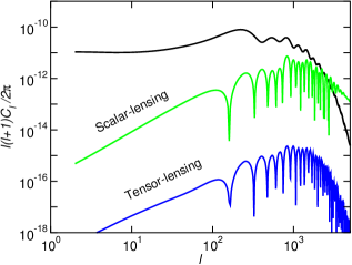
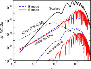
Figure 2: The lensing modification to CMB power spectra for density perturbations and for gravitational waves. Left: Temperature fluctuations. The top curve is the primordial power spectrum. The middle curve is the (additive) contribution to the temperature power spectrum from lensing by density perturbations, and the lower curve is for lensing by gravitational waves, assuming the maximum IGW background consistent with current CMB bounds. Note that for the lower two curves, it is $|\tilde{C}_{l}-C_{l}|$ which is plotted. The negative contribution of the $R$ term in Eq. (5) allows for $\tilde{C}_{l}-C_{l}$ to become negative. Since the coherence scale for $C_{l}^{\Omega\Omega}$ is so small, the lensed power spectrum reflects closely at high $l$ the primordial temperature power spectrum. Right: Polarization. These curves are: (1) the top (solid) curve is the primordial E-mode power spectrum; (2) the next-highest (solid) curve is the lensing correction to the primordial E-mode power spectrum by density perturbations; (3) the top dashed curve is the B-mode power spectrum resulting from cosmic-shear conversion of E-modes by density perturbations; (4) the lower dashed curve is the B-mode power spectrum from lensing by foreground IGWs; and (5) the lowest solid curve is the E-mode power spectrum resulting from lensing by foreground IGWs. The dot-dash curve is the primordial B power spectrum from the maximal IGW background allowed by current constraints.

IV.2 Second-order density perturbations

Gravitational lensing by density perturbations can give rise to a curl component once we go to second order in the projected potential $\phi$. To see this, we first review the lowest-order effect. Suppose there is a lens at a distance $r_{1}$ along the line of sight. The deflection by this lens is $\delta\theta_{i}\propto\partial_{i}\Phi_{1}$, where $\Phi_{1}$ is the gravitational potential (not the projected potential) at $r_{1}$. The lowest-order deflection will therefore be written as the sum of gradients perpendicular to the line of sight. To second order in $\Phi$, there can be deflection by two lenses at different distances, $r_{1}$ and $r_{2}$, along the line of sight. The deflection by the first lens the ray encounters is $\propto\partial_{j}\Phi_{1}$, and the deflection after encountering the second lens is $\propto(\partial_{i}\partial_{j}\Phi_{2})(\partial_{j}\Phi_{1})$ (this follows from the discussion, e.g., in Section 3 of Ref. CooHu02 ). To see that this has nonvanishing curl, we take the curl: $\epsilon_{ik}\partial_{k}[(\partial_{i}\partial_{j}\Phi_{2})(\partial_{j}\Phi_{1})]\propto\epsilon_{ik}(\partial_{i}\partial_{j}\Phi_{2})(\partial_{j}\partial_{k}\Phi_{2})$ which does not generally vanish.

The full calculation of the curl power spectrum is then lengthy but straightforward, and it is discussed in the context of galaxy-based weak lensing surveys in Ref. CooHu02 . They are explored in the context of CMB lensing in Ref. HirSel03 . We do not repeat the derivation but refer the reader to Ref. CooHu02 for details.

V Calculations and Results

A comparison of the gravitational-wave and density-perturbation (to second order) curl signals to the gradient lensing signal is shown in Fig. 1. [Note that the anisotropy spectra for the lensing convergence and rotation are related to the gradient and curl by $C_{l}^{\kappa\kappa}=(l^{4}/4)C_{l}^{\phi\phi}$ and $C_{l}^{\omega\omega}=(l^{4}/4)C_{l}^{\Omega\Omega}$.] Here, we push the gravitational-wave amplitude to the maximum allowed by current data. A useful measure of the relative importance of the two components is the rms deflection angle on the sky given by $\theta^{2}_{\rm rms}=\int[d^{2}{\bf l}/(2\pi)^{2}]l^{2}C_{l}^{XX}$. In the case of density perturbations (for $X=\phi$), $\theta_{\rm rms}=7\times 10^{-4}$ or roughly $2.5$ arcmins. The angular coherence scale, where the rms drops to half its peak value, is about a degree. In the case of the strongest gravitational wave background, the deflection angle is $\theta_{\rm rms}=7\times 10^{-5}$ or 0.25 arcmins, but the angular coherence scale is a few tens of degrees. (Note that the $y$ axis in Fig. 1 is $l^{6}C_{l}$, so the power spectra plotted there are in fact very rapidly falling with $l$. The rms deflection angle is thus fixed primarily by the low $l$’s.) In the case of second-order curl corrections, the coherence scale is similar to that of density perturbations but the amplitude is smaller by at least four to five orders of magnitude. The resulting corrections to CMB anisotropies trace that of the density field, but with a similar reduction in the overall amplitude.

The effects on the CMB anisotropy spectra are summarized in Fig. 2. In the case of temperature, the gravitational-wave-lensing correction is at least two orders of magnitude below the temperature fluctuations associated with the angular displacement corrections due to the density field. We also summarize our results for the case involving polarization anisotropies. In accord with Ref. Dodetal03 , we conclude that the correction resulting from the curl component is negligibly small.

We now turn to the reconstruction of the cosmic-shear pattern with quadratic estimators for $\phi$ and $\Omega$. Fig. 3 shows the errors in the reconstruction for a hypothetical CMB experiment with a resolution of an arcminute and a noise-equivalent temperature of 1 $\mu$K sec^1/2 over one year of integration. We show the reconstruction for both temperature maps (top lines), and for the EB quadratic combination which was shown in Ref. HuOka02 to be the best combination to extract lensing information from CMB data. Note that one generally reconstructs the gradient and curl components of the deflection field with roughly the same signal-to-noise ratio. The gradient component, however, dominates since it is sourced by the large-scale mass distribution, while the curl component is subdominant given that the amplitude of the tensor contribution to the CMB quadrupole is limited by current CMB data to be less than $30\%$ of that due to scalar perturbations.

Figure 3: Reconstructed unbinned noise spectra using the temperature-temperature quadratic estimator and the EB polarization combination. We show noise for both grad and curl modes. For reference, we also plot the power spectrum of the deflection angle corresponding to the gradient component.

VI The Curl as a Diagnostic

Is it useful to reconstruct the curl component as there is virtually no signal? Here, we suggest that a reconstruction may be useful to identify non-Gaussian signals, both due to primary effects, such as primordial non-Gaussianity Les04 or perhaps variable fine-structure constant kris , and secondary anisotropies. As discussed above, although the thermal SZ effect can can be removed largely from multifrequency data cooray , the kinetic-SZ effect cannot. Such an unsubtracted secondary contribution to CMB fluctuations will give rise to an additional noise-bias term in Eq. (13), whereby

$$\langle\hat{X}({\bf l})\hat{X}({\bf l}^{\prime})\rangle=(2\pi)^{2}\delta({\bf l}+{\bf l}^{\prime})(C_{l}^{XX}+N_{l}^{X}+S_{l}^{X})\,.$$ (25)

When secondary non-Gaussianities are not properly accounted for, the additional noise-bias term takes the form

$$S_{l}^{X}=\left(N_{l}^{X}\right)^{2}$$ (26)

$$\times \int\frac{d^{2}{\bf l}_{1}}{(2\pi)^{2}}\int\frac{d^{2}{\bf l}_{2}}{(2\pi)^{2}}\frac{\left\{({\bf l}\odot{\bf l}_{1})C^{\Theta}_{l_{1}}+[{\bf l}\odot({\bf l}-{\bf l}_{1})]C^{\Theta}_{|{\bf l}-{\bf l}_{1}|}\right\}}{2C_{l_{1}}^{\rm t}C_{|{\bf l}-{\bf l}_{1}|}^{\rm t}}$$

$$\times \frac{\left\{({\bf l}\odot{\bf l}_{2})C^{\Theta}_{l_{2}}+[{\bf l}\odot({\bf l}-{\bf l}_{2})]C^{\Theta}_{|{\bf l}-{\bf l}_{2}|}\right\}}{2C_{l_{2}}^{\rm t}C_{|{\bf l}-{\bf l}_{2}|}^{\rm t}}$$

$$\times \langle\Theta^{s}({\bf l}_{1})\Theta^{s}({\bf l}-{\bf l}_{1})\Theta^{s}({\bf l}_{2})\Theta^{s}(-{\bf l}-{\bf l}_{2})\rangle\,,$$

where $\langle\Theta^{s}({\bf l}_{1})\Theta^{s}({\bf l}-{\bf l}_{1})\Theta^{s}({\bf l}_{2})\Theta^{s}(-{\bf l}-{\bf l}_{2})\rangle$ is the four-point correlator of the contaminant foreground or primordial non-Gaussianity with its anisotropy written in Fourier-space as $\Theta^{s}({\bf l})$. This correlator can be decomposed as

$$\langle\Theta^{s}({\bf l}_{1})\Theta^{s}({\bf l}-{\bf l}_{1})\Theta^{s}({\bf l}_{2})\Theta^{s}(-{\bf l}-{\bf l}_{2})\rangle$$

$$=2C^{ss}_{l_{1}}C^{ss}_{|{\bf l}-{\bf l}_{1}|}\delta({\bf l}_{1}+{\bf l}_{2})$$

$$+T^{s}({\bf l}_{1},{\bf l}-{\bf l}_{1},{\bf l}_{2},-{\bf l}-{\bf l}_{2}).$$ (27)

The Gaussian piece leads to a noise bias

$$S_{l}^{X} = \left(N_{l}^{X}\right)^{2}$$

$$= \times\int\frac{d^{2}{\bf l}_{1}}{(2\pi)^{2}}\frac{\left\{({\bf l}\odot{\bf l}_{1})C^{\Theta}_{l_{1}}+[{\bf l}\odot({\bf l}-{\bf l}_{1})]C^{\Theta}_{|{\bf l}-{\bf l}_{1}|}\right\}^{2}}{\left[2C_{l_{1}}^{\rm t}C_{|{\bf l}-{\bf l}_{1}|}^{\rm t}\right]^{2}}$$

$$\times 2\,C^{ss}_{l_{1}}C^{ss}_{|{\bf l}-{\bf l}_{1}|}\,,$$ (28)

which can be absorbed into $N_{l}^{X}$ with a proper definition of the normalization factor, and where $C_{l}^{\rm tot}$ also include foregrounds and secondary power spectra. However, the non-Gaussian nature of the foreground cannot be ignored and this results in a bias that cannot be removed by a renormalization. This noise is,

$$S_{l}^{X} = \left(N_{l}^{X}\right)^{2}\int\frac{d^{2}{\bf l}_{1}}{(2\pi)^{2}}\int\frac{d^{2}{\bf l}_{2}}{(2\pi)^{2}}$$ (29)

$$\times \frac{\left\{({\bf l}\odot{\bf l}_{1})C^{\Theta}_{l_{1}}+[{\bf l}\odot({\bf l}-{\bf l}_{1})]C^{\Theta}_{|{\bf l}-{\bf l}_{1}|}\right\}}{2C_{l_{1}}^{\rm t}C_{|{\bf l}-{\bf l}_{1}|}^{\rm t}}$$

$$\times \frac{\left\{({\bf l}\odot{\bf l}_{2})C^{\Theta}_{l_{2}}+[{\bf l}\odot({\bf l}-{\bf l}_{2})]C^{\Theta}_{|{\bf l}-{\bf l}_{2}|}\right\}}{2C_{l_{2}}^{\rm t}C_{|{\bf l}-{\bf l}_{2}|}^{\rm t}}$$

$$\times T^{s}({\bf l}_{1},{\bf l}-{\bf l}_{1},{\bf l}_{2},-{\bf l}-{\bf l}_{2})\,.$$

The angular dependence of the foreground trispectrum is important: if the trispectrum were to depend on the length of the vectors alone, the averaging would result in significant suppression of this noise bias.

In the presence of an additional secondary trispectrum, for lensing reconstruction,

$$\langle\hat{\phi}({\bf l})\hat{\phi}({\bf l}^{\prime})\rangle=(2\pi)^{2}\delta({\bf l}+{\bf l}^{\prime})(C_{l}^{\phi\phi}+N_{l}^{\phi}+S_{l}^{\phi})\,.$$ (30)

While $N_{l}^{\phi}$ can be established based on noise properties, one cannot separate the signal $C_{l}^{\phi\phi}$ of interest from the confusion $S_{l}^{\phi}$. Such a situation has already been observed, for example, in numerical simulations of the CMB lensing reconstruction process where in the presence of a kinetic-SZ component an additional noise bias was suggested Amb04 . The presence of such a noise bias was readily detectable given that the input mass spectrum, or alternatively the cosmology, was known a priori. In the real case, one is interested in measuring these quantities from the mass spectrum determined from CMB lensing. Thus, the presence of a noise bias cannot easily be established since the bias is degenerate with other unknowns.

The curl component, however, provides a useful method to establish the presence of such a noise bias which can be used to correct the gradient component or to allow for an accounting of the bias when cosmological parameters are measured. This follows from the fact that all signals of interest in the curl component are negligibly small such that the resulting reconstruction only leads to

$$\langle\hat{\Omega}({\bf l})\hat{\Omega}({\bf l}^{\prime})\rangle = (2\pi)^{2}\delta({\bf l}+{\bf l}^{\prime})(N_{l}^{\Omega}+S_{l}^{\Omega})\,.$$ (31)

Since $N_{l}^{\Omega}$, like $N_{l}^{\phi}$ can be predicted from the measured CMB power spectra, any excess noise in the reconstruction will suggest either systematics or the presence of an additional non-Gaussian signal that is contributing via $S_{l}^{\Omega}$. Even though the excess noises in the gradient and curl of the deflection field are different—i.e., $S_{l}^{\Omega}$ vs $S_{l}^{\phi}$—the origin of the excess noise could very well be the same with the only differences resulting from variations in the two filters for the two modes. In general, any detection of excess noise in the curl component should suggest a bias in the gradient component. Since filter shapes are known a priori, one should be able to establish some estimate on the expected excess noise in the gradient, given the excess noise in the curl. If this excess noise is significant, then the dominance of a systematic effect in the reconstruction is clearly established. Currently, there is no mechanism to either estimate or establish the presence of a systematic noise component in the CMB lensing analysis. Thus, we suggest that the curl component be used as a monitor of systematic effects and to understand if the $C_{l}^{\phi\phi}$ reconstruction is affected through $S_{l}$ by non-Gaussian secondary effects and foregrounds.

In general, we do not expect effects such as primordial non-Gaussianity Les04 to be a significant concern for lensing reconstruction of the deflection-potential statistics. Given the noise levels to the reconstruction, as shown in Fig. 3, one can establish the minimum amplitude for which systematic effects or additional noise biases, as described by $S_{l}$, can be detected via

$$\sigma_{A}^{-2}=\sum_{l}\frac{1}{\sigma_{l}^{2}}\left(\frac{\partial S_{l}}{\partial A}\right)^{2}\,.$$ (32)

Here $\sigma_{l}=\sqrt{2/(2l+1)}N_{l}$, under the assumption of no signal in the curl component. Using the estimated noise levels, from the EB combination of polarization maps to reconstruct the curl component, for example, one can establish systematic effects down to a level of 0.1% from the amplitude of the potential-fluctuation power spectrum. In the cosmic-shear simulations of Ref. Amb04 , noise biases at the level of 30% or more were found. We surmise that some of this may be due to conversion of kinetic-SZ corrections to a deflection angle, although this probably does not account for all the excess noise. A study of the curl component may help clarify the nature of such noise biases in the simulation.

VII Summary

Lensing by gravitational waves is expected to give rise to a cosmic-shear pattern where the deflection angle has a curl (or transverse-vector) component, as opposed to the curl-free pattern expected by cosmic shear by density perturbations (to linear order in the perturbation amplitude). To second order in the perturbation amplitude, lensing can also give rise to a curl component. For a primordial background of gravitational waves from inflation with a normalization given by the current upper limit to the tensor-to-scalar ratio, the corrections to the CMB power spectra are generally two orders of magnitude below those of the cosmic shear due to density perturbations, and the curl component from higher-order lensing effects is also small. The curl component can be reconstructed with quadratic estimators analogous to those developed to measure the gradient component. Given the small signal expected in the curl, this component can potentially be used as a probe of systematic effects and foregrounds for next-generation CMB experiments

- (1) See, e.g., U. Seljak and M. Zaldarriaga, Phys. Rev. Lett. 82, 2636 (1999) [arXiv:astro-ph/9810092]; Phys. Rev. D 60, 043504 (1999) [arXiv:astro-ph/9811123]; M. Zaldarriaga and U. Seljak, Phys. Rev. D 59, 123507 (1999) [arXiv:astro-ph/9810257]; W. Hu, Phys. Rev. D 64, 083005 (2001) [arXiv:astro-ph/0105117].
- (2) W. Hu, Phys. Rev. D 62, 043007 (2000) [arXiv:astro-ph/0001303].
- (3) W. Hu, Astrophys. J. Lett. 557, L79 (2001) [arXiv:astro-ph/0105424].
- (4) W. Hu and T. Okamoto, Astrophys. J. 574, 566 (2002) [arXiv:astro-ph/0111606].
- (5) M. Kesden, A. Cooray, and M. Kamionkowski, Phys. Rev. D 67, 123507 (2003) [arXiv:astro-ph/0302536].
- (6) C. M. Hirata and U. Seljak, Phys. Rev. D 68, 083002 (2003) [arXiv:astro-ph/0306354].
- (7) M. Kesden, A. Cooray, and M. Kamionkowski, Phys. Rev. Lett. 89, 011304 (2002) [arXiv:astro-ph/0202434]; L. Knox and Y.-S. Song, Phys. Rev. Lett. 89, 011303 [arXiv:astro-ph/0202286]; U. Seljak and C. Hirata, Phys. Rev. D 69, 043005 (2004) [arXiv:astro-ph/0310163].
- (8) R. D. Blandford et al., Mon. Not. Roy. Astron. Soc. 251, 600 (1991); J. Miralda-Escudé, Astrophys. J. 380, 1 (1991); N. Kaiser, Astrophys. J. 388, 277 (1992); M. Bartelmann and P. Schneider, Astron. Astrophys. 259, 413 (1992).
- (9) D. J. Bacon, A. R. Refregier, and R. S. Ellis, Mon. Not. Roy. Astron. Soc. 318, 625 (2000) [arXiv:astro-ph/0003008]; N. Kaiser, G. Wilson, and G. A. Luppino, Astrophys. J. 556, 601 (2001) [arXiv:astro-ph/0003338]; D. M. Wittman et al., Nature 405, 143 (2000) [arXiv:astro-ph/0003014]; L. van Waerbeke et al., Astron. Astrophys. 358, 30 (2000) [arXiv:astro-ph/0002500].
- (10) A. Stebbins, arXiv:astro-ph/9609149.
- (11) G. Luppino and N. Kaiser, Astrophys. J. 475, 20 (1997) [arXiv:astro-ph/9601194] ; A. Stebbins, T. McKay, and J. Frieman, in Astrophysical Applications of Gravitational Lensing, eds. C. Kochanek and J. Hewitt, (Kluwer Academic Press, Dordrecht, 1996) [arXiv:astro-ph/9510012]; M. Kamionkowski et al., Mon. Not. Roy. Astron. Soc. 297, 486 (1998) [arXiv:astro-ph/9712030].
- (12) A. Cooray and W. Hu, Astrophys. J. 574, 19 (2002) [arXiv:astro-ph/0202411].
- (13) S. Dodelson, E. Rozo, and A. Stebbins, Phys. Rev. Lett. 91, 021301 (2003) [arXiv:astro-ph/0301177].
- (14) M. Kamionkowski, A. Kosowsky, and A. Stebbins, Phys. Rev. Lett. 78, 2058 (1997) [arXiv:astro-ph/9609132]; U. Seljak and M. Zaldarriaga, Phys. Rev. Lett. 78, 2054 (1997) [arXiv:astro-ph/9609169].
- (15) R. A. Sunyaev and Ya. B. Zel’dovich, Mon. Not. Roy. Astron. Soc. 190, 413 (1980).
- (16) K. Sigurdson, A. Kurylov, and M. Kamionkowski, Phys. Rev. D 68, 103509 (2003) [arXiv:astro-ph/0306372].
- (17) N. Kaiser and A. H. Jaffe, Astrophys. J. 484, 545 (1997) [arXiv:astro-ph/9609043].
- (18) J. R. Pritchard and M. Kamionkowski, arXiv:astro-ph/0412581.
- (19) A. Melchiorri and C. J. Odman, Phys. Rev. D 67, 021501 (2003) [arXiv:astro-ph/0210606].
- (20) J. Lesgourgues, M. Liguori, S. Matarrese and A. Riotto, arXiv:astro-ph/0412551.
- (21) A. Cooray, W. Hu, and M. Tegmark, Astrophys. J. 540, 1 (2000) [arXiv:astro-ph/0002238].
- (22) A. Amblard, C. Vale, and M. J. White, New Astron. 9, 687 (2004) [arXiv:astro-ph/0403075].