Early structure in $\Lambda$CDM

Abstract

We use a novel technique to simulate the growth of one of the most massive progenitors of a supercluster region from redshift $z\sim 80$, when its mass was about $10{\rm M_{\odot}}$, until the present day. Our nested sequence of $N$–body resimulations allows us to study in detail the structure both of the dark matter object itself and of its environment. Our effective resolution is optimal at redshifts of 49, 29, 12, 5 and 0 when the dominant object has mass $1.2\times 10^{5}$, $5\times 10^{7}$, $2\times 10^{10}$, $3\times 10^{12}$ and $8\times 10^{14}h^{-1}{\rm M_{\odot}}$ respectively, and contains $\sim 10^{6}$ simulation particles within its virial radius. Extended Press-Schechter theory correctly predicts both this rapid growth and the substantial overabundance of massive haloes we find at early times in regions surrounding the dominant object. Although the large-scale structure in these regions differs dramatically from a scaled version of its present-day counterpart, the internal structure of the dominant object is remarkably similar. Molecular hydrogen cooling could start as early as $z\sim 49$ in this object, while cooling by atomic hydrogen becomes effective at $z\sim 39$. If the first stars formed in haloes with virial temperature $\sim 2000$K, their comoving abundance at $z=49$ should be similar to that of dwarf galaxies today, while their comoving correlation length should be $\sim 2.5h^{-1}$Mpc.

Early structure in $\Lambda$CDM

1 Introduction

Within the cold dark matter (CDM) paradigm for structure formation, first light in the Universe is usually assumed to have come from stars which collapsed early at the centres of rare and unusually massive dark matter haloes associated with high peaks of the initial gaussian overdensity field. Soon after their birth, these stars began to influence the structure, the thermodynamics and the chemical content of surrounding gas. The epoch when this occurred and the precise details of how it happened are not yet well understood.

Recent simulations including gravitational, chemical and radiative processes have suggested that metal-free gas in dark matter haloes of virial temperature ${\rm T_{vir}\sim 2000K}$ and mass ${\rm M}\sim 10^{6}{\rm M_{\odot}}$ cooled efficiently by emission from molecular hydrogen and collapsed to form a star at redshifts $18<z<30$. (Abel et al. 1998, 2002; Fuller & Couchman 2000, Bromm et al. 2002; Yoshida et al. 2003; for reviews see Bromm & Larson 2004 and Glover 2004). To achieve the required resolution, these calculations followed evolution within very small cubic subvolumes of the Universe assuming periodic boundary conditions. Such boundary conditions suppress all fluctuations with wavelength longer than the side of the simulated region. As we shall see, this can have drastic effects, particularly on the morphology of large-scale structure and on the abundance and formation history of objects with mass more than roughly $10^{-4}$ of the total mass in the simulated region.

In fact, the first haloes of any given mass (and thus quite probably the first stars) do not form in “typical” regions at all, but rather in “protocluster” regions (White & Springel 2000; Barkana & Loeb 2004). This is an effect of the relatively large contribution from Mpc wavelengths to the fluctuation amplitude on even the smallest mass scales, and is reflected, for example, in the plots presented by Mo & White (2002) for the spatial clustering strength of haloes for redshifts out to $z\sim 20$. Conclusions about early objects reached from simulations of small and “typical” regions may thus be misleading; in particular, the formation redshift of the first haloes of any given mass or temperature will be systematically underestimated. An alternative strategy is to simulate regions which are constrained to have high overdensity or to contain a high amplitude density peak (Abel et al. 1998, Fuller & Couchman 2000; Bromm et al. 2002) but this leads to interpretational difficulties because there is no clear relation between the statistical properties of the resulting objects and those of the rare objects of similar mass which would form from unconstrained initial conditions (White 1996).

The formation of the first stars has also been studied by combining semi-analytical modelling of baryonic processes (e.g. Tegmark et al 1997; Hutchings et al. 2002; Yoshida et al. 2003) with Press-Schechter or extended Press-Schechter predictions of the number density of dark matter haloes (Press & Schechter 1974; Bond et al. 1991; Bower 1991; Lacey & Cole 1993, 1994). Over the limited mass range that they test, recent N-body simulations have shown that the halo number density in the concordance cosmology is reasonably well matched by the Sheth & Tormen (1999) variant of the Press-Schechter model (Jenkins et al. 2001; Reed et al. 2003; Yahagi et al. 2004; Gao et al. 2004a, Springel et al. 2005). Unfortunately, this work is still far from testing the regime that is relevant for studies of the first stars.

In this paper, we attempt to simulate an example of one of the first haloes capable of forming stars. Anticipating that these will be progenitors of massive present-day objects, we perform a series of nested resimulations of the most massive progenitor of a rich cluster and its supercluster environment. In each resimulation we increase the resolution, we include additional small-scale structure in the initial conditions, and we start at higher redshift in order to capture the early phases of nonlinear evolution. As anticipated from the above discussion, we find that our simulated halo would likely form its first star at significantly higher redshifts than suggested by previous work. In this paper, however, we simulate only the formation and evolution of the dark halo itself. A more detailed consideration of baryonic processes is deferred to a companion paper (Reed et al. 2005c) and to later papers which include simulation of hydrodynamics and radiative cooling.

Our paper is structured as follows. In Section 2, we describe our simulation sequence, the methods used to set up initial conditions, to integrate the equations of motion, and to identify haloes, and the evolution in mass and effective abundance of the dominant object. In Section 3, we present images of our main halo and its immediate surroundings at $z=49,29,12,5$ and $0$. We also present density profiles and an analysis of substructure for this halo at these same times, and we chart its remarkably rapid growth in virial temperature. Internal structure is surprisingly similar at different times, whereas halo environment changes systematically and qualititively with increasing redshift. In Section 4 we extend our study of environment to larger scales, highlighting the qualitative difference in structure between early and late times. At redshift 50 the dark matter distribution in our simulation is very different from a scaled copy of that at $z=0$. In this section we also compare the number density of haloes in our simulations with analytical models, showing that there is an extremely strong clustering bias which is quite well modelled by a suitable version of extended Press-Schechter theory. In Section 5, we discuss the some possible implications of our calculations for the formation on the first stars. Finally, we summarize our conclusions in Section 6.

2 Simulations details

We adopt standard values for the cosmological parameters. For the mean densities of dark matter, dark energy and baryons (in units of the critical density) we take $\Omega_{\rm DM}=0.26$, $\Omega_{\Lambda}=0.7$ and $\Omega_{\rm B}=0.04$ respectively. The present value of the Hubble parameter is set to $h=0.7$ and the extrapolated linear amplitude of fluctuations in a sphere of radius $8h^{-1}{\rm M}_{\odot}$ is set to $\sigma_{8}=0.9$. We computed the initial linear power spectrum down to $k\sim 2000h{\rm Mpc}^{-1}$ using CMBFAST with a primordial spectral index $n=1$ (Seljak & Zaldarriaga, 1996). It was necessary to extrapolate a further order of magnitude in wavenumber to reach the Nyquist frequency corresponding to our highest resolution resimulation. This was done using a power-law matched to the slope ($dn/dlnk=-2.99$) at the join. Strictly speaking, there should be some curvature, but at these wavenumbers the slope is very close to its asymptotic value of $-3$.

2.1 The simulations

Table 1: Numerical parameters for the R series simulations

	$R1$	$R2$	$R3$	$R4$	$R5$
$N_{p}$	8457516	5804755	8658025	41226712	73744737
$m_{p}[h^{-1}{\rm M_{\odot}}]$	$5.12\times 10^{8}$	$2.2\times 10^{6}$	$1.24\times 10^{4}$	$29.5$	$0.545$
$\epsilon[h^{-1}{\rm kpc}]$	5.0	0.8	0.15	0.017	0.0048
$M_{200}[h^{-1}{\rm M_{\odot}}]$	$8.1\times 10^{14}$	$4.6\times 10^{12}$	$2.0\times 10^{10}$,	$5.2\times 10^{7}$	$1.2\times 10^{5}$
$r_{200}[h^{-1}{\rm kpc}]$	1514.1	401.5	65.9	9.1	1.2
$z_{i}$	39	149	249	399	599
$z_{f}$	0.0	5.0	12.04	29.04	48.84

It is a challenge to simulate the formation of early structure in a CDM universe because the first collapsed objects are very small. In addition, the slope of the matter power spectrum at high wavenumber approaches the critical value $-3$ for which equal contributions to the variance of the density field come from each logarithmic interval in wavenumber. Thus a very wide range of scales must be included in order to simulate correctly the early formation of small objects. The required dynamic range is beyond present algorithms and computer resources by a wide margin so it is currently impossible to carry out simulations with sufficient resolution everwhere to follow the nonlinear dynamics of the first collapsing structures.

We have devised a multigrid procedure which circumvents this problem and allows us to follow the growth of an object in its full cosmological context from $z=80$ to $z=0$. Over this period its mass increases by about 13 orders of magnitude. The procedure works as follows:

(1)

We identify a rich cluster halo at $z=0$ in a cosmological simulation of a very large volume.

(2)

We resimulate the evolution of this rich cluster and its environment with much higher mass and force resolution, while following the remainder of the simulation volume at lower resolution than before. We ensure the proper treatment of small-scale structure by starting the resimulation at higher redshift than the original, and including in its initial conditions a random realisation of the fluctuations at wavenumbers between the Nyquist frequencies of the original and the higher resolution particle distributions.

(3)

We find the most massive object in the high resolution region of this resimulation at each redshift and identify the time when it first contains more than about 10000 particles within its virial radius.

(4)

We then resimulate the evolution of this progenitor object and its immediate surroundings with further improved mass and force resolution, while again following the more distant matter distribution at lower resolution.

(5)

We iterate steps 3 and 4 until we reach the desired redshift and progenitor mass.

In practice, we chose at random a rich cluster of virial mass $8\times 10^{14}h^{-1}{\rm M_{\odot}}$ from the VLS simulation of the Virgo consortium, a cosmological simulation of a cubic region of side $479h^{-1}$Mpc (Jenkins et al. 2001, Yoshida et al. 2001). The first resimulation of this cluster involved a single application of the “zoom” technique first introduced by Navarro & White (1994) in the implementation described and tested by Power et al. (2003). This was one of the cluster resimulations analyzed in Navarro et al. (2004) and Gao et al. (2004a,b,c). For the present paper we repeated this “zoom” step four more times reaching ever higher mass and force resolution. We thus have a total of 5 resimulations in addition to the original VLS simulation. We label these R1 ($z_{f}=0$), R2 ($z_{f}=5$), R3($z_{f}=12$), R4 ($z_{f}=29$) and R5 ($z_{f}=49$), where $z_{f}$ is both the final redshift of each resimulation and the redshift at which the most massive progenitor in the high-resolution region of the previous resimulation was identified. We checked the virial mass of the main object and the morphology of the surrounding structure between each pair of simulations at these times, finding excellent agreement in all cases. The first object to reach a mass greater than 10000 particles in the high-resolution region of R1 turned out not to be a progenitor of the main cluster itself, but rather of a smaller $\sim 10^{14}h^{-1}{\rm M_{\odot}}$ member of the same $z=0$ supercluster. At $z=5$, this object was $15$ per cent more massive than the most massive progenitor of the main cluster. The objects resimulated in R3, R4 and R5 did, however, all turn out to be progenitors of this same object.

The high resolution regions of the first three resimulations, R1–R3, had final radii about $4$ times the virial radius of the final massive object. For R4 and R5 we chose to follow a more extended region in order to investigate the large-scale environment of the principal halo. The first three resimulations used the original periodic boundaries of the parent VLS simulation. For R4 and R5 we used isolated boundary conditions with sharp spherical cuts at comoving radii of $5h^{-1}$Mpc and $1.25h^{-1}$Mpc respectively. At the relevant redshifts the universe is quite homogeneous on these scales, and our target objects were almost unaffected by the omission of more distant structure. Note that this cut-off, unlike the imposition of periodic boundary conditions, does not exclude the contribution to the density field due to long wavelength modes, although it does significantly affect the bulk motion of the whole simulated region. This is of no consequence here.

Further details of our series of resimulations are listed in Table 1. Here $N_{p}$ is the total number of particles in the high resolution region of each resimulation, $m_{p}$ is the mass of each of these particles, $\epsilon$ is the gravitational softening parameter (in comoving units), $M_{200}$ is the mass of the final object within the sphere of radius $r_{200}$ (also given in comoving units) which encloses a mean overdensity of $200$ relative to critical, and $z_{i}$ and $z_{f}$ are the initial and final redshifts of each resimulation.

In most of our resimulations the dominant halo at the final time has about 2 million particles inside $r_{200}$. Only for R5 at $z=49$ was this number significantly lower, about $0.2$ million. For this highest resolution resimulation, the particle mass was $0.5h^{-1}{\rm M_{\odot}}$ and the force softening $5h^{-1}$pc in comoving units. The growth in mass of the principal object we have followed is shown in the first panel of Figure 1. (As noted above, after $z\sim 4$ this is not the most massive object in the high resolution region of R1.) The rapidity with which the mass increases at early times is quite remarkable. Picking a series of redshifts separated by factors of two in expansion factor, we find masses of $10^{3}h^{-1}{\rm M}_{\odot}$ at $z=63$, of $2\times 10^{7}h^{-1}{\rm M}_{\odot}$ at $z=31$, of $5\times 10^{9}h^{-1}{\rm M}_{\odot}$ at $z=15$, of $4\times 10^{11}h^{-1}{\rm M}_{\odot}$ at $z=7$, of $7\times 10^{12}h^{-1}{\rm M}_{\odot}$ at $z=3$, of $3\times 10^{13}h^{-1}{\rm M}_{\odot}$ at $z=1$, and of $10^{14}h^{-1}{\rm M}_{\odot}$ at $z=0$.

For given halo mass and redshift, one can define a characteristic abundance as the mean number of haloes of equal or greater mass per unit volume in the Universe as a whole. While our iterative procedure is guaranteed to find a rare, massive halo at high redshift, the corresponding abundance cannot be estimated directly from our resimulations since these focus on “special” regions. It cannot be much lower than the $z=0$ abundance of galaxy clusters like that initially selected, and in fact it turns out to be significantly higher. Nevertheless, only an extremely small fraction of all cosmic mass is locked up in objects as massive as the one we are tracking.

We illustrate these points in the lower two panels of Figure 1 using the Sheth & Tormen (1999) formulae to estimate abundance and mass fraction. Note that these estimates require extrapolation far beyond the regime in which these formulae have been numerically tested; while undoubtedly qualitatively correct, they may contain significant errors beyond $z\sim 10$. At $z\sim 50$ the comoving abundance of objects like the one we have simulated is predicted to be similar to that of $10^{11}{\rm M_{\odot}}$ haloes today, but such objects contain only a few times $10^{-7}$ of all cosmic matter, corresponding approximately to $5.9\sigma$ peaks of the initial gaussian density field. In contrast, the rich cluster we originally selected corresponds only to a $2.7\sigma$ peak, while the $z=0$ descendent of our high redshift halo corresponds to an even less rare $1.7\sigma$ peak. It is interesting that a large excursion is visible at $z\sim 5$ in the plots of Figure 1, which explains how the progenitor of the $10^{14}{\rm M_{\odot}}$ object managed to “beat out” that of the more massive $z=0$ cluster we had originally chosen. In addition, there is a clear change in behaviour in some of these plots after this redshift which is related to the fact that the object is no longer subject to the condition that it must evolve into an extreme system at later times (see also Figure 4 below).

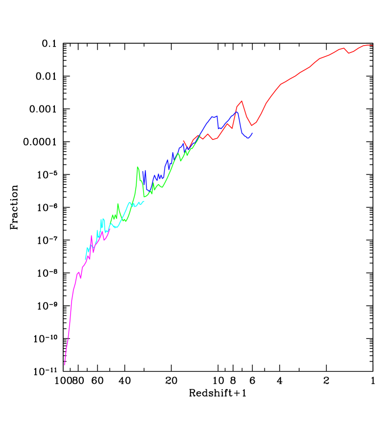
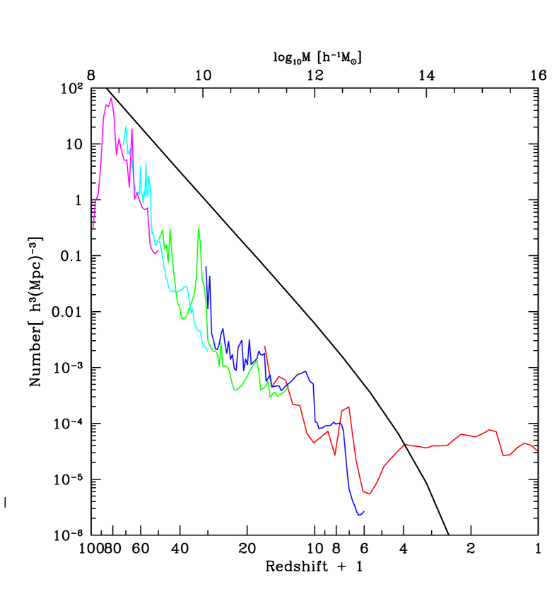
Figure 1: (Top) The mass $M_{200}$ of the object we have followed since its first progenitor was detected (at $z\sim 80$) until the present day. Different line-types represent our different resimulations. The smooth curve is predicted using extended Press-Schechter theory and is discussed in section 4.2. (Lower left) The fraction of all cosmic mass which at redshift $z$ is in haloes with mass exceeding that plotted in the top panel. (Lower right) The comoving cosmic abundance of haloes at least as massive as our dominant object. The results in the two lower panels are based on the formulae of Sheth &Tormen (1999). The thick solid line in the lower right panel is the cumulative halo abundance at at $z=0$ predicted by these same formulae and should be compared with the mass scale at the top of the plot.

Our R1 resimulation was carried out with the publicly available tree code GADGET-1.1 (Springel, Yoshida & White 2001). Our other resimulations used an improved TREE-PM code GADGET-2 (Springel 2005).

2.2 Halo identification

Two of the most common methods for identifying haloes in $N$-body simulations are the friends-of-friends (FOF) algorithm of Davis et al. (1985), and the spherical overdensity (SO) algorithm described by Lacey & Cole (1994). Advantages of FOF are that it does not impose any fixed shape on the haloes, and that it is fast. However, it occasionally links separate haloes over a chance bridge of particles, and the most massive haloes in a large simulation are often such multiple objects. In the limit of large particle number, FOF haloes are approximately bounded by an isodensity contour.

In the SO algorithm, the mass of a halo is evaluated in a spherical region. There is only one free parameter, the mean overdensity $\delta$ within this region. There are, however, many possible ways to determine its centre. For practical purposes, most of these are equivalent. In our implementation, the centre is determined iteratively. A local maximum of the density field, estimated by the standard SPH method, is taken as an initial guess. A sphere is then grown outward until it reaches the desired mean overdensity. The centre-of-mass of this sphere is taken as the next guess at the centre and the procedure is repeated. After several iterations, the motion of the centre becomes small. The SO algorithm rarely identifies haloes with multiple major concentrations, but it is slower than the FOF algorithm and it does impose a fixed spherical shape when determining halo masses

As we shall see in later sections, the first massive objects are found in overdense regions containing many smaller haloes which line up along filaments and sheets. In this situation we find that the FOF halo identification algorithm is quite dependent on the mass resolution of the simulation. For example, using a linking length of 0.2 times the mean interparticle separation (at the cosmic mean density), the halo mass functions in corresponding regions at $z=49$ of the R4 and R5 resimulations are very different; $19$ per cent of all high resolution particles are identified as a single halo in R5, but the most massive halo is much smaller in R4. On the other hand, as can be seen in Fig. 2, the abundance of haloes selected by SO assuming $\delta=180$ (again relative to the cosmic mean) agrees well in the two resimulations down to the resolution limit of R4. In the following we use the SO(180) algorithm to identify all haloes, unless otherwise stated, although we often quote masses and radii as $M_{200}$ or $r_{200}$ referring to a spherical region with mean density 200 times the critical value.

Figure 2: Halo mass functions at $z=49$ for the common region of the R4 and R5 simulations. Haloes were identified and their masses estimated using the SO(180) algorithm. Error bars show Poisson uncertainties in the counts for the R4 haloes.

3 The evolution of extreme haloes

In this section we study the growth of the main halo in our simulation sequence and consider how its internal structure changes with time. We wish to test whether the halo and its environment at high redshift are similar to a suitably scaled version of low redshift structures. It has often been argued that dark matter evolution should be effectively self-similar in hierarchical clustering. This could only be strictly true in an Einstein-de Sitter universe with a power-law initial fluctuation spectrum (e.g. Efstathiou et al. 1988; Smith et al. 2003). Some deviations are expected in the concordance $\Lambda$CDM cosmology, both because of the influence of the cosmological constant at low redshift, and because of the curvature of the initial power spectrum. In addition, the fact that the power spectrum slope approaches the critical value $-3$ at high wavenumber implies a breakdown at early times of the critical assumption underlying the hierarchical clustering model, namely that small things form first. Our sequence of resimulations provides an opportunity to explore whether these effects lead to qualitatively different behaviour at early times. We begin by displaying images of the main halo and its immediate surroundings at the end of each of our resimulations. These are the times when the structure is best resolved. Subsequent subsections consider the evolution in characteristic temperature, in density profile and in substructure content of the principal halo.

3.1 Images

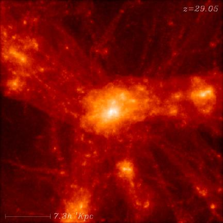
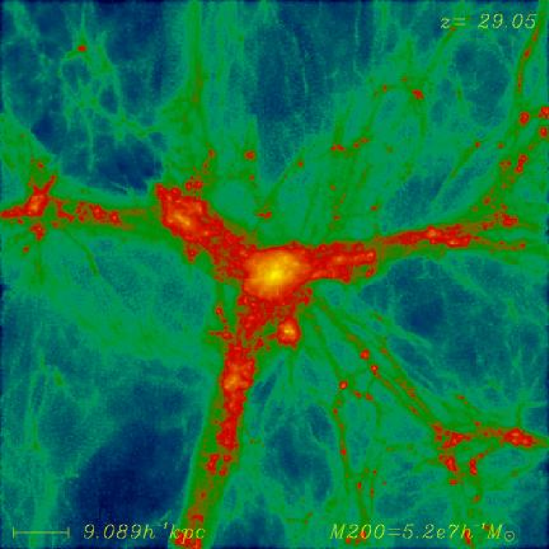
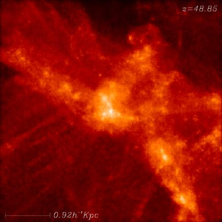
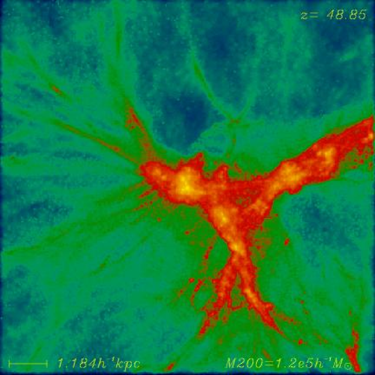
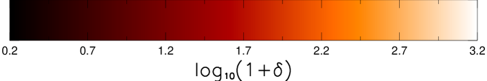
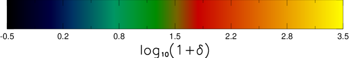
Figure 3: Projected dark matter density in and around the most massive haloes present at the final time of each of our resimulations. The left-hand panels show the dark matter distributions within cubes of side $4r_{200}$ centred on the main halo. The right-hand panels show distributions in slices $10r_{200}$ on a side and $2r_{200}$ thick, also centred on the main halo. In each image, the density field is normalized to the projected mean cosmic density and depicted on a logarithmic scale. The colour scales are identical at the different times in each series of images but differ between the left and right series.

The distribution of dark matter in and around the most massive halo at the end of each of our resimulations is illustrated in Fig. 3. Note again that the $z=0$ halo is not the descendent of the haloes shown at earlier times. The left-hand column depicts one projection of the density in a cube of side $4\times r_{200}$ centred on the main halo. (In comoving units, $r_{200}$ ranges from $1.5$ Mpc for the R1 halo at $z=0$ to $1.2$ kpc for the R5 halo at redshift $z=49$; see Table 1.) The surface density is normalized to the cosmic mean and the color table represents the dimensionless surface density, $1+\delta$, on a logarithmic scale. In all cases, a centrally concentrated object is clearly visible at the centre of the image, but as the redshift increases the matter distribution becomes increasingly anistropic. At $z=12$ and earlier very strong filaments surround the central halo and appear less fragmented into individual smaller objects than at later times.

The right-hand column of Fig. 3 illustrates the larger scale environment of these main haloes. The images here have side $10r_{200}$, are projections of a region of depth $2r_{200}$, and again all represent the projected overdensity using an identical colour scale. The qualitative change in morphology with redshift is more dramatic in these plots. As we go back in time the main halo becomes less dominant and less regular, the “filamentary” structures become heavier and smoother, and substructure both within and outside the main object becomes less evident. At the earliest times, the filaments extend over the full region plotted and are the most striking structure within it. Note that with the exception of the latest pair ($z=5$ and $z=0$) all the matter shown in each early image is contained within the central object of the next later one.

3.2 The growth in halo temperature

The rapid growth in mass of our principal halo was already shown in the top panel of Fig. 1. At each time we can estimate a representative temperature for the gas associated with this halo from its maximumum circular velocity, $V_{c}$:

$$T=\mu m_{p}V_{c}^{2}/(2k_{B})\,$$ (1)

where $\mu m_{p}$ is the mean molecular weight of the gas and $k_{B}$ is Boltzmann’s constant. This “virial” temperature is plotted as a function of redshift in Fig. 4. We assume $\mu=1.22$ from the earliest redshift until the temperature has risen to $10000$K. At this time we assume that the gas is collisionally ionised and has $\mu=0.59$ thereafter; during the transition the halo temperature is taken to be constant at ${\rm T}_{\rm Vir}=10000$K. Like the mass, the halo temperature increases very rapidly at early times. Already by $z=49$, it has reached $\sim 2000$K when, for the high densities predicted at these redshifts, molecular hydrogen should form sufficiently rapidly to provide efficient radiative cooling. As many recent simulations have shown, this is likely to lead to the formation of a massive star at the centre of our object (Abel et al 1998, 2002; Bromm et al. 2002; Yoshida et al. 2003). The critical temperature for collisional ionisation $T\sim 10^{4}$K is reached by $z=39$ and the greatly increased efficiency of cooling at this point could lead to a starburst and the formation of a minigalaxy. Whether this actually happens depends on the evolution of the first star. Its ionising radiation and the strong shock it produces if it goes supernova could already have affected surrounding gas over a large region by $z=39$ (e.g. Yoshida, Bromm &Hernquist 2004). We study these issues as well as others associated with the formation of the first stars in a companion paper (Reed et al. 2005c).

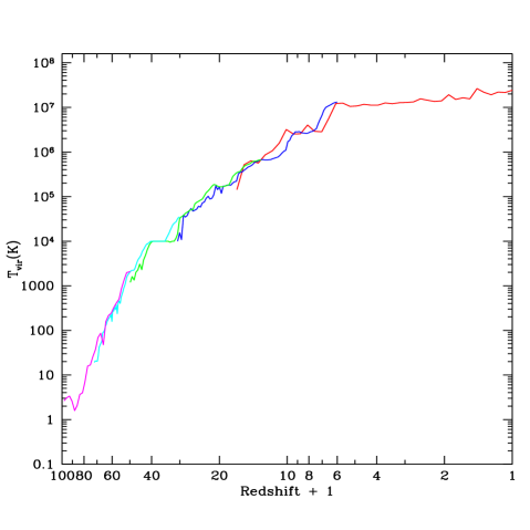
Figure 4: Increase with time of the characteristic temperature (estimated from the maximum circular velocity) of the principal halo in our sequence of resimulations.

3.3 The evolution of halo density profiles

Simulations of structure formation in hierarchical clustering cosmogonies (including the concordance $\Lambda$CDM model) produce dark matter haloes with density profiles which can be fit by the simple formula proposed by Navarro, Frenk & White (1996, 1997; NFW),

$$\rho(r)={\rho_{s}\over(r/r_{s})(1+(r/r_{s})^{2}}.$$ (2)

Here $r_{s}$ is a characteristic radius where the profile declines locally as $r^{-2}$, and $\rho_{s}/4$ is the density at $r_{s}$. At the relatively low redshifts where this formula has been tested, there is a strong correlation between $r_{s}$ and $\rho_{s}$ which depends on redshift, on the global cosmological parameters, and on the initial power spectrum. The larger the mass of a halo, the lower its characteristic density, reflecting the lower density of the universe at the (later) time when more massive systems were typically assembled. The applicability of this formula in the innermost regions of haloes has been controversial, but recent work suggests that it is a reasonable fit to most haloes over the radial range $0.01r_{200}<r<r_{200}$; the behaviour at yet smaller radii remains a topic of debate (Navarro et al. 2004; Reed et al. 2005a; Diemand et al. 2004).

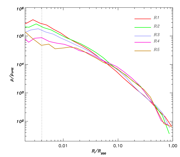
Figure 5: Density profiles for the final halo in each resimulation. Open squares show the mean density within spherical shells plotted against shell radius. Both axes are given in physical (rather than comoving) units. The solid lines are fits to an NFW profile and weight each point outside the gravitational softening radius equally. They imply the concentration parameters $c=r_{200}/r_{s}$ given in each panel. Dashed vertical lines show the gravitational softening in each resimulation. The five profiles are superposed in the bottom right plot after scaling radii to $r_{200}$ and densities to the critical density. This emphasises the evolution of shape with redshift.

Roughly two million particles lie within the virial radius of the final halo in all our resimulations except R5, whose halo has only $\sim 220000$ particles within $r_{200}$. The density profiles are very well sampled and this allows us to investigate the internal structure of these extreme objects as a function of redshift. In Fig. 5 we show the density profile of the most massive halo in each resimulation at the final time, together with the best-fit NFW profile. The NFW formula is a good fit to the data over the full range plotted at the three later times. At $z=29$ and $z=49$, however, the fits are quite poor; the profiles are shallower than the analytic formula at small radii and steeper at large radii.

In the lower right-hand panel of the figure, we superpose the density profiles so that their shapes can be compared. When scaled by $r_{200}$, the profiles vary systematically with redshift, their inner slope and concentration decreasing with increasing redshift. Note that the profiles in R1 and R2 are quite similar, as are the profiles in R4 and R5. The profile in R3 is intermediate in behaviour. The R4 and R5 profiles look qualitatively different from the others, reinforcing the impression from the images in Figure  3. These changes presumably reflect the very steep spectrum of the $\Lambda$CDM cosmology and the resultant very rapid growth of structure on these small mass scales.

3.4 Substructure in early haloes

The high resolution achieved by N-body simulations in recent years has enabled detailed study of the substructure expected within dark haloes in the standard cosmogony (Ghigna et al. 2000; De Lucia et al. 2004; Diemand et al. 2004b,Gao et al. 2004a,b). Subhaloes are the surviving cores of objects which fell together during the hierarchical assembly of the halo, and it is natural to attempt to relate their number and properties to observed substructures such as individual galaxies within galaxy clusters (Springel et al. 2001b) or satellite galaxies within the haloes of Milky Way-like systems (Klypin et al. 1999; Moore et al. 1999). Unfortunately, both observational and theoretical arguments show the correspondence between subhaloes and galaxies to be quite complicated and to depend strongly on the history of the subhaloes rather than just on their mass and position (Springel et al. 2001b; Stoehr et al. 2002; Gao et al. 2004a,b; Nagai & Kravtsov, 2005).

Because of the extremely rapid build-up of the main object in our resimulation sequence and the relatively smooth appearance of the structure that surrounds it at early times, it might seem a priori likely that substructure should be less prominent in early haloes than in low redshift systems. Figure 6 demonstrates that this is not the case. We plot the cumulative subhalo mass function for the most massive halo at the final time in each of our resimulations. Masses are normalised to the value of $M_{200}$ for the massive halo and only subhaloes within $r_{200}$ are included. The subhaloes here were identified using the SUBFIND algorithm described in Springel et al (2001b). Remarkably, the substructure mass function is very similar at all redshifts except $z=0$. Subhaloes in the massive cluster halo in R1 are roughly a factor of 1.5 more abundant at given mass fraction than at earlier times.

The radial distribution of subhaloes within the parent halo is less concentrated than that of the mass as a whole and is quite similar at all epochs. The cumulative profiles of Fig. 7) are plotted for subhaloes with at least 30 particles, the limit to which Gao et al. (2004a) considered this distribution to be insensitive to resolution effects; the profiles found here are all similar to those shown in this earlier paper.

It seems therefore that within $r_{200}$ the internal structure of the most massive haloes present at high redshift (radial profile, abundance and radial distribution of subhaloes) differs relatively little from that of present-day rich cluster haloes, despite the large differences in dimensionless assembly rate and in the morphology of the structures from which they form.

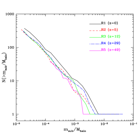
Figure 6: Cumulative subhalo mass functions for the most massive halo at the final time in each of our sequence of resimulations.

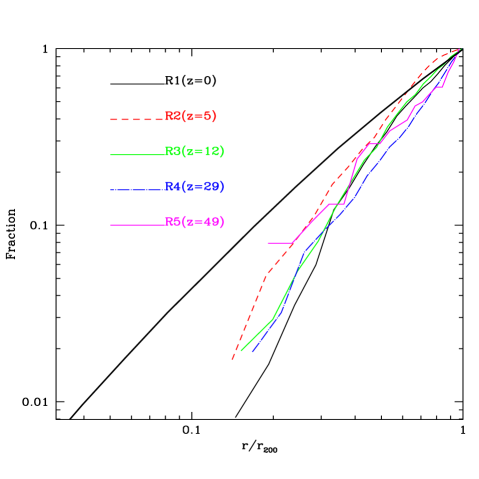
Figure 7: Cumulative radial number density profiles for subhaloes of the most massive halo at the final time in each of our sequence of resimulations. Only subhaloes within $r_{200}$ and consisting of at least 30 particles are considered. The smooth heavy line is the corresponding distribution for the total mass of the R1 halo.

4 Large-scale structure at high redshift

4.1 Morphology

The fundamental hypothesis underlying the hierarchical clustering paradigm is that small objects collapse first and gradually aggregate into larger systems. This requires that the linear power spectrum of mass density fluctuations at the beginning of the matter-dominated phase of cosmic evolution should, in a power-law approximation, be $P(k)\propto k^{n}$ with $n>-3$. At late times when large galaxies, clusters and superclusters are forming, the effective index of the standard $\Lambda$CDM power spectrum is in the range $-2<n<0$ and structure growth is indeed hierarchical. At the early times we are studying here, however, the effective index on the scales dominating nonlinear growth is very close to $-3$ and an “orderly” hierarchical build-up is not guaranteed. This is reflected in the very rapid early growth of the object we have focussed on, and we may expect the simultaneous collapse of structure on a very wide range of scales to produce a different morphology for large-scale structure than is seen at later times. The image of structure at $z=17$ presented by Yoshida et al. (2003; their Figure 1) certainly looks quite different from the familiar pictures of low redshift large-scale structure.

In this subsection we compare large-scale structure at $z=49$ and at $z=0$. By construction our resimulations are centred on a rare and massive object. We therefore compare structure in the high-resolution region of R4 to structure surrounding our massive cluster in the VLS simulation. It is unclear how the two models should be scaled to carry out this comparison, since, for any reasonable definition of the nonlinear mass scale, it is many orders of magnitude smaller at $z=49$ than at $z=0$. We have chosen to scale, as in Fig. 3, by the characteristic size $r_{200}$ of the central object. Since our $z=49$ object is, in a dimensionless sense, much rarer than our $z=0$ object (i.e. farther out on the tail of the mass distribution; see the mass fraction plot of Figure 1) one might expect $r_{200}$ for the high-redshift object to be larger than that of an object which “correctly” corresponds to the $z=0$ halo. We would then underestimate the factor by which early large-scale structure should be magnified in order to correspond to $z=0$ structure. In fact, however, the opposite is true: even with the scaling we have chosen, large-scale structure is much more coherent at $z=49$ than at $z=0$.

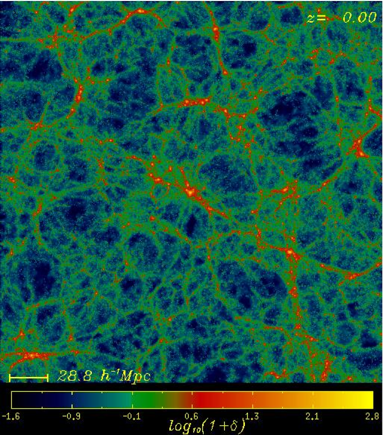
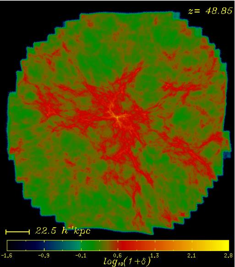
Figure 8: Projected dark matter density fields at $z=49$ and at $z=0$ in slices centred on a rare and massive halo. The side of each plot is $190r_{200}$ and its thickness is $10r_{200}$ where $r_{200}=1.2h^{-1}$kpc in comoving units for the central halo at $z=49$ and $r_{200}=1.5h^{-1}$Mpc for the central halo at $z=0$. The left-hand plot is taken from the parent VLS simulation and is centred on the rich cluster halo chosen for our series of resimulations. The right-hand plot shows the high resolution region of R4 and is centred on the main halo which was resimulated in R5. The density fields are normalized in each case by the mean projected cosmic density at the corresponding epoch and they are displayed using the same logarithmic colour scale in the two plots.

In Fig. 8, we compare large-scale structure at $z=49$ and $z=0$ after applying this scaling. The regions shown are $190r_{200}$ on a side and are $10r_{200}$ in depth. We have normalised by the projected mean cosmic density at each epoch and used the same logarithmic colour scale to display the two images. The qualitative and quantitative differences between the two plots are dramatic. The mean overdensity across the whole image at $z=49$ is clearly substantially higher than at $z=0$, and in fact the mean density of the high resolution region of R4 at the redshift plotted is more than 2.5 times the global cosmic mean, even though the mass in this region is five orders of magnitude larger than that of the central halo. In addition, the large-scale structure at $z=49$ has a single dominant peak and extends more or less coherently across the whole region, while at $z=0$ there are many peaks of quite similar mass and morphology to the central one and typical filaments and voids are smaller than the region plotted. Clearly it is dangerous to assume that large-scale structure in the early universe is just a scaled version of that familiar from simulations of low redshift structure formation.

4.2 Biases in the abundance of haloes

The regions followed by our resimulations are not typical regions of the universe, since, by construction, they are centred on a rare and massive object. Indeed, all the material followed at high resolution in R$n$ falls onto this object during the evolution of R$(n-1)$ for $n=2,3,4$ and $5$. It is this bias which is responsible, of course, for the substantial overdensity of the whole $z=49$ region plotted in Fig. 8, and it results in accelerated growth of objects throughout the overdense region in comparison with “typical” regions of the universe. This may be quantified by comparing the mass function of haloes in the high resolution regions of our resimulations with that expected at the same redshift for the universe as a whole. Fig. 9 shows, as a function of mass, the abundance of objects identified by the SO(180) algorithm in spherical regions centred on the most massive halo at two different redshifts. The left-hand plot is based on the VLS simulation at $z=0$ and shows results for spheres of radius $80$, $40$ and $20$ times $r_{200}=1.5h^{-1}$Mpc. The right-hand plot is based on R4 at $z=49$ and shows results for spheres with the “same” radii, except that now $r_{200}=1.2h^{-1}$kpc in comoving units. These plots thus correspond to the simulations and redshifts illustrated in Fig. 8.

Both panels of Fig. 9 also show predictions for the halo mass function in “typical” regions of the universe based on the standard Press-Schechter (PS; Press & Schechter 1974) and Sheth & Tormen (ST; Sheth &  Tormen 1999) formulae. At $z=0$ these formulae agree moderately well and the ST prediction, in particular, is very close to the fitting function proposed by Jenkins et al. (2001) as a good representation of the best available simulation data. At $z=49$, however, the two predictions disagree badly – by a factor of about 10 at $1000h^{-1}{\rm M}_{\odot}$ and by a factor of about 100 at $10^{5}h^{-1}{\rm M}_{\odot}$. In this regime there are no reliable simulations with which they can be compared, so it is unclear which (if either) is most correct. For the largest high-resolution simulation of a “typical” region carried out so far, the so-called Millennium Run, the ST formulae continue to fit the high mass tail of the concordance $\Lambda$CDM mass function out to $z=10$ where the PS formulae already underpredict by about an order of magnitude (Springel et al. 2005). Nevertheless, these results are still a factor of 5 in redshift and $10^{6}$ in mass from the regime of concern here.

Both the PS and the ST formula fit the $z=0$ data well for spheres of radius $80$ and $40r_{200}$ and the simulation results in the two cases are indistinguishable. For the sphere of radius $20r_{200}$ , the simulation results are similar at small mass but appear high at the large mass end. Within the two larger spheres the mean overdensity is close to zero, so no substantial bias is expected theoretically. The situation is dramatically different at redshift $z=49$. Even though the ST prediction is much larger than that from PS theory, it still lies far below any of the mass functions measured from the simulation. In addition, the three spheres produce mass functions which differ considerably, with the smallest sphere having the largest abundances. As noted above, the overdensities within these spheres are substantial, and as we now show, their mass functions can be predicted surprisingly well by inserting these overdensities into a suitable version of the conditional or extended Press-Schechter model (EPS; Bond et al. 1991; Bower 1991; Lacey & Cole 1993, 1994; Mo & White 1996).

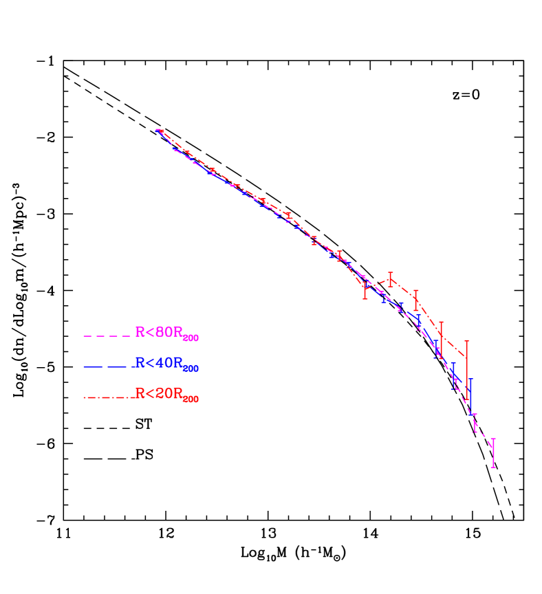
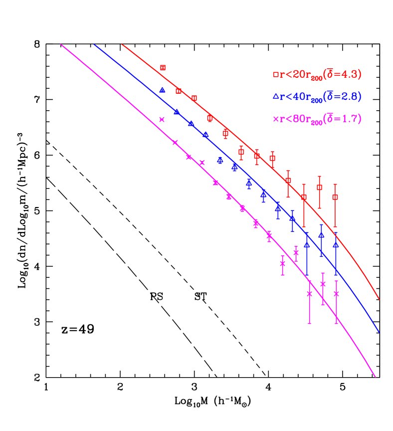
Figure 9: Halo mass functions in the VLS (left) and R4 (right) simulations for spherical regions of radii $80r_{200}$, $40r_{200}$ and $20r_{200}$ centred on the R1 halo at $z=0$ and on the R5 halo at $z=49$. Objects were identified using the SO(180) algorithm. The error bars represent Poisson uncertainties in the counts. In both panels we give predictions based on the PS and ST formulae for the halo abundance in typical regions of the Universe. In the right-hand panel, solid lines show predictions of the extended Press–Schechter model for regions with the measured nonlinear overdensities.

According to the EPS model as worked out by Mo & White (1996), the fraction of the material in a large spherical region of total mass $M_{0}$ and linear overdensity extrapolated to the present day $\delta_{0}$ which, at redshift $z$, is contained in dark haloes with mass in $(M_{1},M_{1}+dM_{1})$, is given by

$$f(M_{1},z|M_{0},\delta_{0})dM_{1}=(\frac{1}{2\pi})^{1/2}\frac{\delta_{1}-\delta_{0}}{(\Delta_{1}^{2}-\Delta_{0}^{2})^{3/2}}$$ (3)

$$\exp[-\frac{(\delta_{1}-\delta_{0})^{2}}{2(\Delta_{1}^{2}-\Delta_{0}^{2})}]\frac{d\Delta_{1}^{2}}{dM_{1}}dM_{1},$$

where $\Delta_{0}$ and $\Delta_{1}$ are the rms linear fluctuations extrapolated to the present day in spheres which on average contain masses $M_{0}$ and $M_{1}$ respectively, and $\delta_{1}$ is the critical linear overdensity for collapse at $z$ also extrapolated to the present day. To evaluate $\delta_{0}$, we must relate the nonlinear overdensity $\delta$ measured at redshift $z$ in Eulerian space to the original linear overdensity in Lagrangian space. Based upon the spherical collapse model, Mo & White(1996) provided an analytical fitting formula which links these two overdensities in an Einstein-de Sitter universe. Sheth & Tormen (2002) later showed that this formula remains reasonably accurate for all cosmologies of interest.

$${}\delta_{0}(\delta,z)\!\!\! = \!\!\!{\delta_{1}\over 1.68647}\times\Biggl{[}1.68647-{1.35\over(1+\delta)^{2/3}}$$ (4)

$$\qquad\qquad\quad-{1.12431\over(1+\delta)^{1/2}}+{0.78785\over(1+\delta)^{0.58661}}\Biggr{]}$$

The nonlinear overdensity in the spherical regions used to make Figure 9 can be estimated straightforwardly from the simulations. For R4 at $z=49$ we find $\delta_{nl}=1.7,2.8$ and $4.3$ for spheres of radius $80r_{200}$, $40r_{200}$ and $20r_{200}$ respectively. For the VLS simulation at $z=0$ the corresponding numbers are -0.02, 0.17 and 0.49. These numbers can be converted to linear overdensities using equations (4), while the radii of the spheres can be converted to Lagrangian radii simply by multiplying by $(1+\delta_{nl})^{1/3}$. Equations (3) then predict the halo abundance in these regions. We plot the results as thick solid lines in the left panel of Fig. 9. (We do not show these curves at $z=0$ since they differ little from the standard PS prediction.) Clearly, the agreement with the measured abundances is very good. Fig. 10 shows that the EPS model works equally well at $z=30$. For this plot we consider the halo abundance in a spherical region of radius $20r_{200}$, the largest sphere that fits completely within the high resolution region of R3 at this redshift. As noted above, tests of the standard PS formula show increasingly poor fits to the high mass tail of the global mass function at high redshift (and, in particular, much worse fits than the ST formula), so it is remarkable that the EPS mass function gives a such an accurate estimate of halo abundance in high density regions at these early times. The redshift and mass ranges tested here, $z=30-50$ and $M\sim 10^{5}-10^{6}{\rm M_{\odot}}$, are those most relevant for the collapse of the haloes which host the first stars.

The EPS formalism may also be used to calculate the growth history of a given halo. At given (high) redshift, we estimate the expected mass of the most massive progenitor of the final halo by integrating the EPS progenitor mass function down from infinity until the expected total number of progenitors is equal to $1$. We then adopt the mean progenitor mass over this range as our estimate for the largest progenitor mass. The thick line in the upper panel of Fig. 1 shows the resulting prediction for the growth in mass of the dominant halo in our resimulation series. (Recall that the final object is not the most massive halo at $z=0$ in R1 but rather a nearby halo of mass $1.07\times 10^{14}h^{-1}{\rm M_{\odot}}$.) Remarkably, the theoretical prediction follows our simulation results very closely, with at most a $10$ per cent shift in redshift at early times. We believe this close agreement to be at least partly fortuitous, since we have also resimulated the most massive $z=5$ progenitor of the rich cluster halo we originally picked from the VLS simulation. Although at $z=5$ it is only 15% less massive than the object we have concentrated on in this paper (and at $z=0$ is a factor $8$ more massive), by $z=29$, the earliest time for which we currently have a reliable mass estimate, it is less massive than our principal object by a factor of $10$. Clearly, there is substantial scatter in growth histories of the kind we are studying.

5 Implications for the formation of the first stars

In the context of the $\Lambda$CDM cosmogony, understanding the formation and evolution of early dark haloes is a prerequisite for understanding the formation of the first stars. Although first star formation depends strongly on additional hydrodynamic and radiative processes, dark halo collapse provides the dynamical context for these processes, and so can serve as a useful guide to when and where the first stars may form. We already saw in Fig. 1 and Fig. 4 that a halo of virial temperature $\sim 2000$K is in place in our simulation series by $z=49$. These are the properties usually suggested as appropriate for the condensation of the first stellar generation through molecular hydrogen cooling. By $z=39$ the biggest halo has high enough temperature for efficient cooling by atomic processes. We now briefly consider the implied abundance and clustering of such objects. A more detailed discussion is given in our companion paper (Reed et al. 2005c).

Figure 10: Differential mass function in a spherical region with radius $20r_{200}$ centred on the most massive halo in our R3 simulation at $z=30$. The solid line shows the prediction from EPS theory. The error bars assume Poisson uncertainties in the counts.

The lower right-hand panel of Figure 1 shows the ST formulae to predict that at $z=49$ the mean abundance of objects at least as massive as our dominant halo is $\sim 10^{-1}h^{3}$Mpc^-3, while at $z=39$ it is $\sim 10^{-2}h^{3}$Mpc^-3. These numbers correspond roughly to the present-day abundance of $10^{11}$ and $10^{12}h^{-1}{\rm M_{\odot}}$ haloes respectively. The lower left-hand panel of Figure 1 demonstrates that only a tiny fraction of all mass is in such haloes, about $2\times 10^{-7}$ at $z=49$ and about $3\times 10^{-6}$ at $z=39$. Since the masses of the first stars are expected to be a few hundred M_⊙, the fraction of all baryons in stars at $z=49$ is predicted to be around $10^{-10}$. This is far too low for their UV flux to reionise a significant fraction of the IGM. These early objects would thus create isolated HII regions with a very small filling factor. Atomic cooling might allow more efficient condensation of the baryons into stars in the $z=39$ objects, but even then the abundance is too low for the HII regions to percolate. In addition, activity related to a central star formed at $z\sim 49$ might eject the baryons from these objects before their virial temperature reaches the critical value for atomic cooling.

Closely related to the fact that the main progenitors of high-mass objects accrete matter very rapidly at high redshift is the fact that the abundance of objects above a given (high) mass or temperature threshold increases very rapidly with time. Thus while the ST prediction for the mass fraction in objects with virial temperature above 2000K is $2\times 10^{-7}$ at $z=49$, it has already increased to $3\times 10^{-5}$ by $z=39$ with a corresponding abundance of $\sim 10h^{3}$Mpc^-3, well above that of dwarf galaxies today. Note that these strong dependences are also reflected in considerable sensitivity of these ST predictions to the particular form used for the $\Lambda$CDM power spectrum. Here, as in our simulations, we have used the spectrum given by CMBFAST (Seljak & Zaldarriaga 1996). In the regime we are considering, switching to the analytical fits quoted by Bond & Efstathiou (1987) or Bardeen et al. (1986) alters the abundance at fixed halo mass and redshift by up to an order of magnitude, and the redshift at fixed halo mass and abundance by up to $\Delta z\sim 5$.

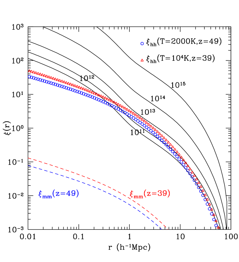
Figure 11: Halo auto-correlation functions. Open circles show $\xi_{hh}$ for haloes of virial temperature 2000K at $z=49$, while open triangles refer to 10000K haloes at $z=39$. Solid lines are predictions for $z=0$ haloes with the masses noted. All these functions were calculated using the procedures of Mo & White (1996). For comparison, the dashed lines show the correlation functions predicted for the mass distribution at $z=49$ and $z=39$.

A final point of interest for the first stars is the spatial clustering of their potential host haloes. This has a direct impact on the likelihood that a star or star cluster can affect star formation in neighbouring haloes. It also has consequences for the morphology of the IGM during its reionisation and so for the form of the predicted signal in future redshifted 21cm surveys (e.g. Ciardi & Madau 2003). The halo autocorrelation function is easily estimated using the formalism proposed by Mo & White (1996) which is based upon the EPS and top-hat collapse models and was tested by them against direct N-body simulations. The halo auto-correlation function, $\xi_{hh}(r)$, is given by

$$\xi_{hh}(r,M,z)=b^{2}(M,z)\xi_{mm}(r,z)~{}.$$ (5)

where

$$b(M,z)=1+\frac{\nu^{2}(M,z)-1}{\delta_{c}(z)},~{}~{}~{}\nu=\delta_{c}(z)/\Delta(M),$$ (6)

is the bias factor for haloes of mass $M$ at redshift $z$ (Cole & Kaiser 1989; Mo & White 1996, 2002; Jing 1998), and $\xi_{mm}$ is the nonlinear auto-correlation function of the underlying mass, estimated to sufficient accuracy from the linear power spectrum by the procedure of Peacock & Dodds (1996). Equation 5 is only valid on scales significantly larger than the size of the haloes, and, like the PS and ST formulae, it has not been tested numerically in the regime where we use it here. In Fig. 11, we compare the correlation functions for 2000K haloes at $z=49$ and for 10000K haloes at $z=39$ with those for haloes with a variety of masses today. (Note that lengths in this plot are in comoving units.) The halo correlation amplitudes at these early times are several hundred times that of the underlying mass. On scales of a few Mpc they are comparable to that of $M\sim 10^{12}h^{-1}{\rm M_{\odot}}$ dark haloes today. The correlation length (defined by $\xi(r_{0})=1$) is $r_{0}=2.5h^{-1}$Mpc for our $z=49$ haloes and is $r_{0}\sim 3h^{-1}$Mpc for the $z=39$ haloes. Thus on Mpc scales, the comoving clustering pattern of the first stars and galaxies may be quite similar to that of dwarf galaxies today.

6 Conclusions

We have invented a novel strategy which allows us to follow the build-up of a massive object within the concordance $\Lambda$CDM cosmogony over an unprecedentedly large range in redshift and mass. In the particular resimulation series presented in this paper we track the growth of one particular object from a mass of about $10h^{-1}{\rm M_{\odot}}$ at $z=80$ to about $10^{14}h^{-1}{\rm M_{\odot}}$ at the present day. Throughout the series the full cosmological environment of the object is correctly represented so we can study evolution both of its internal structure and of the “large-scale” structure in which it is embedded. As a by-product we are able to estimate approximately when the baryons associated with this particular object would first have been able to collapse to form a star. Our main results may be summarized as follows:

(1)

Massive objects at early times accrete mass extremely rapidly and form in regions where the overdensity is high on much larger scales than those of the objects themselves.

(2)

At early times ($z\geq 12$) the filamentary structure surrounding the massive objects is much stronger than at lower redshifts ($z\leq 5$).

(3)

At very high redshift ($z\sim 50$) large-scale structure is qualitatively different from that in the low redshift universe. In particular the characteristic size of coherent structures is much larger in relation to the typical size of collapsed objects.

(4)

Despite this, the internal structure of massive early dark haloes is quite similar to that to their present-day counterparts, both in terms of density profiles and in terms of substructure. Although early objects are less concentrated and have less substructure, the differences are relatively small.

(5)

The number density of haloes in overdense regions at high redshift is surprisingly well described by the extended Press-Schechter model, at least in the redshift interval $z=50-30$ that we study here.

(6)

By $z=49$ our main object has reached virial temperature $2000$K and should soon form sufficient molecular hydrogen for gas to condense into a central massive star. Pockets of star formation may thus have appeared much earlier than previously thought. At $z=49$ such 2000K haloes have a comoving number density comparable to that of $\sim 10^{11}h^{-1}{\rm M_{\odot}}$ haloes today, but by $z=40$ this has already increased by almost two orders of magnitude. By $z=39$ our main halo has a virial temperature of 10000K so its gas can start cooling by atomic processes and turning, perhaps, much more efficiently into stars.

(7)

Over the redshift range $30<z<50$ haloes like the one we have simulated have comoving correlation lengths up to $3h^{-1}$Mpc, similar to those of present-day dwarf galaxies. The ionisation and dissociation structures their associated stars produce is studied in our companion paper (Reed et al. 2005c).

By clarifying how the dark matter distribution evolves in and around extreme objects, our simulations set the scene for the more complex processes of gas cooling, collapse and fragmentation that result in the first stars. We will study these processes in forthcoming papers using direct simulation of the baryonic component.

References

- [Abel et al. (1998)] Abel T., Anninos P., Norman M. L., Zhang Y., 1998, 508, 518
- [Abel et al. (2002)] Abel T., Bryan G., Norman M. L., 2002, science, 295, 93
- [Bardeen et al. (1986)] Bardeen J. M., Bond J. R., Kaiser N., Szalay A. S., 1986, ApJ, 304, 15
- [Barkana &Loeb (2004)] Barkana R., Loeb A., 2004, ApJ, 609, 474
- [Bond &Efstathiou (1987)] Bond J. R., Efstathiou G., 1987, MNRAS, 226, 655
- [Bond et al. (1991)] Bond J. R., Cole S., Efstathiou G., Kaiser N., 1991, ApJ, 379, 440
- [Bower (1991)] Bower R. G., 1991, MNRAS, 248, 332
- [Bromm et al. (2005)] Bromm V., Larson R. B., 2004, ARA&A, 42, 79
- [Bromm et al. (2002)] Bromm V., Coppi, P. S., Larson R. B., 2002, ApJ, 564, 23
- [Davis et al. (1985)] Davis M., Efstathiou G., Frenk C. S., White S. D. M., 1985, MNRAS, 292, 371
- [Lucia et al. (2004)] De Lucia G., Kauffmann G., Springel V., White S. D. M, Lanzoni, B., Stoehr, F., Tormen, G., Yoshida, N., 2004, MNRAS, 348, 333
- [Diemand et al. (2004)] Diemand, J., Moore, B., Stadel, J., 2004, MNRAS, 353, 624
- [Efstathiou et al. (1988)] Efstathiou G., Frenk C. F., White S. D. M., Davis M., 1988, MNRAS, 235, 715
- [Gao et al. (2004a)] Gao L., Loeb A., Peebles P. J. E., White S. D. M., Jenkins A., 2004a, ApJ, 614, 17
- [Gao et al. (2004b)] Gao L., White S. D. M., Jenkins A., Stoehr F., Springel V., 2004b, 355, 819
- [Gao et al. (2004c)] Gao L., De Lucia G., White S. D. M., Jenkins A., 2004c, MNRAS, 352, L1
- [Ghigna et al. (2000)] Ghigna S., Moore B., Governato F., Lake G., Quinn T., Stadel J., 2000, ApJ, 544, 616
- [Glover (2005)] Glover S. C. O., 2005, preprint, astro-ph/0409737
- [Fuller et al. (2000)] Fuller T. M., Couchman H. M. P., 2000, ApJ, 544, 6
- [Hutchings et al. (2002)] Hutchings R. M., Santoro F., Thomas P. A., Couchman H. M. P., 2002, MNRAS, 330, 927
- [Jenkins et al. (2001)] Jenkins A., Frenk C.S., Pearce F.R., Thomas P.A., Colberg J.M., White S. D. M., Couchman H. M. P., Yoshida N., 2001, MNRAS, 321, 372
- [Jing et al. (1998)] Jing Y. P., 1998, ApJ, 503, 9
- [Klypin et al. (1999)] Klypin A., Kravtsov A. V., Valenzuela V., Prada F., 1999, ApJ, 522, 82
- [Lacey &Cole (1993)] Lacey C., Cole S., 1993, MNRAS, 262, 627
- [Lacey &Cole (1994)] Lacey C., Cole S., 1994, MNRAS, 271, 676
- [Mo &White (1996)] Mo H. J., White S. D. M., 1996, MNRAS, 282, 347
- [MO &White (2002)] Mo H. J., White S. D. M., 2002, MNRAS, 336, 112
- [Moore et al. (1999)] Moore B., Ghigna S., Governato F., Lake G., Quinn T., Stadel J., Tozzi P., 1999 ApJ, 524, 19
- [Nagai et al. (2005)] Nagai D., Kravtsov A. V., 2005, MNRAS, 618, 557
- [Navarro & White (1994)] Navarro J. F., White S. D. M., 1994, MNRAS, 267, 401
- [Navarro, Frenk &White (1996)] Navarro J. F., Frenk C. F., White S. D. M., 1996, ApJ, 462, 563
- [Navarro et al. (1997)] Navarro J. F., Frenk C. S., White S. D. M., 1997, ApJ, 490, 493
- [Navarro et al. (2004)] Navarro J. F., Hayashi E., Power C., Jenkins A., Frenk C. F., White S. D. M., Springel V., Stadel J., Quinn T. R., 2004, MNRAS, 349, 1039
- [Peacock &Dodds (1996)] Peacock J. A., Dodds S. J., 1996, MNRAS, 280, 19
- [Power et al. (2002)] Power C., Navarro J. F., Jenkins A., Frenk C. S., White S. D. M., Springel V., Stadel J., Quinn T., 2003, MNRAS, 338, 14p
- [Reed et al. (2003)] Reed D. et al., 2003, MNRAS, 346, 565
- [Reed et al. (2005a)] Reed D. et al., 2005a, MNRAS, 357, 82
- [Reed et al. (2005b)] Reed D., Governato F., Quinn T., Gardner J., Stadel J., Lake G., 2005b, MNRAS, 359, 1537
- [Reed et al. (2005c)] Reed D., Bower R., Frenk C. S., Gao L., Jenkins A., Theuns T., White S. D. M., 2005c, MNRAS submitted, astro-ph/0504038
- [Seljak et al. (1996)] Seljak U., Zaldarriaga M., 1996, ApJ, 469, 437
- [Sheth et al. (1999)] Sheth R., Tormen G.,1999, MNRAS, 308,119
- [Sheth & Tormen (2002)] Sheth, R. K., Tormen, G., 2002, MNRAS, 329, 61S
- [Smith et al. (2003)] Smith R. E., Peacock J. A., Jenkins A., White S. D. M., Frenk C. S., Pearace F. R., Thomas P. A., Efstathiou G., Couchman H. M. P.(The Virgo consortium), 2003, MNRAS, 341, 1311S
- [Springel et al. (2001)] Springel V., Yoshida N., White S. D. M., 2001, New Ast. 6, 79
- [Springel et al. (2001)] Springel V., White S. D. M., Tormen G., Kauffmann G., 2001b, MNRAS, 328, 726
- [Springel et al. (2005)] Springel V., White S. D. M., Jenkins A., Frenk C., Yoshida N., Gao L. et al, 2005, Nature, 435, 629
- [Springel (2005)] Springel V. 2005, MNRAS submitted, astro-ph/0501304
- [Stoehr et al. (2002)] Stoehr F., White S. D. M., Tormen G., Springel V., 2002, MNRAS, 335, 762
- [White (1996)] White S. D. M., 1996, in Schaeffer R., Silk J., Spiro M., Zinn-Justin J., eds, Cosmology and Large Scale Structure, Les Houches Session LX. Elsevier, Amsterdam, P.77 s
- [White &Springel] White S. D. M, Springel V., 2000, The first stars, Springer-Verlag: Berlin, P. 327
- [Yoshida et al. (2001)] Yoshida N., Sheth R. K., Diaferio A., 2001, MNRAS, 328, 669
- [Yoshida et al. (2003)] Yoshida N., Abel T., Hernquist L., Sugiyama N., 2003, ApJ, 592, 645
- [Yoshida et al. (2004)] Yoshida N., Bromm V., Hernquist L., ApJ, 605, 579