New supersymmetric partners for the
associated Lamé potentials

Abstract

We obtain exact solutions of the one-dimensional Schrödinger equation for some families of associated Lamé potentials with arbitrary energy through a suitable ansatz, which may be appropriately extended for other such a families. The formalism of supersymmetric quantum mechanics is used to generate new exactly solvable potentials.

Keywords: Supersymmetric quantum mechanics, associated Lamé potentials

PACS: 11.30.Pb, 03.65.Ge, 03.65.Fd

1 Introduction

The solution of the one-dimensional Schrödinger equation with periodic potentials is important due to the possibility of finding interesting models which could be used in physics. This kind of potentials admits a spectrum composed of allowed energy bands, in which the physical eigenfunctions are bounded, separated by energy gaps, where the eigenfunctions are unbounded and thus they cannot have physical meaning due to their exponential growing when we move far away from a given position.

Of special interest are the so-called exactly solvable problems which, unfortunately, in the periodic case include very few potentials, e.g., Lamé and some others. To be precise, by exact solvability we mean that for the corresponding potential it is possible to determine analytically the physical eigenfunctions for energies in the allowed bands (the edges included), as well as the non-physical solutions for energies in the gaps. It is important to notice that in the direct spectral problems the unphysical solutions are neglected because they are apparently useless. However, in the inverse spectral problems, which somehow include the supersymmetric quantum mechanics as a particular case [1, 2], they can be used as seeds to generate exactly solvable potentials from a given initial one [3, 4, 5, 6, 7, 8].

In recent times it has been realized that the associated Lamé potentials, which include in particular the Lamé case, admit explicit expressions for the band edge eigenfunctions [9, 10, 11, 12, 13]. Thus, it is natural to explore if those potentials are exactly solvable in the sense pointed above. If the answer turns out to be positive, then the band edge eigenfunctions as well as the non-physical solutions for the gaps can be used through supersymmetric quantum mechanics to generate new exactly solvable potentials, some of which could provide some interesting physical information.

In the next section we will consider some particular families of the associated Lamé potentials and show that they belong to the exactly solvable class. Then, the formalism of supersymmetric quantum mechanics will be applied to generate new exactly solvable potentials. We will end the paper with our conclusions.

2 Associated Lamé potentials: general solutions

The Schrödinger equation for the associated Lamé potentials in Jacobi form may be expressed as

$$-\frac{d^{2}\psi(x)}{dx^{2}}+V(x)\psi(x)=E\psi(x),\qquad x\in\mathbb{R},$$

$$V(x)=m(m+1)k^{2}{\rm sn}^{2}x+\ell(\ell+1)k^{2}\frac{{\rm cn}^{2}x}{{\rm dn}^{2}x}.$$ (1)

Our aim is to find exact solutions of Eq. (1) for arbitrary values of $E$. Here ${\rm sn}x\equiv{\rm sn}(x,k),\ {\rm cn}x\equiv{\rm cn}(x,k),\ {\rm dn}x\equiv{\rm dn}(x,k)$ are three Jacobian elliptic functions of real modulus $k^{2}\ (0<k^{2}<1)$ and of double periods $4K,2iK^{\prime};4K,4iK^{\prime};$ $2K,4iK^{\prime}$ respectively, $K=\int_{0}^{\pi/2}d\phi/\sqrt{1-k^{2}\sin^{2}\phi}$ is called complete elliptic integral of second kind and $K^{\prime}\>=\int_{0}^{\pi/2}d\phi/\sqrt{1-k^{\prime 2}\sin^{2}\phi}$, $k^{\prime 2}=1-k^{2}$ is known as complementary modulus. In the first step of the process we express Eq. (1) in Weierstrass form to easily observe the difference from the Lamé potential:

$$-\frac{d^{2}\psi}{dz^{2}}+\left[m(m+1)\wp(z)+\frac{\ell(\ell+1)\bar{e}_{2}\bar{e}_{3}}{\wp(z)-e_{1}}\right]\psi=\tilde{E}\psi,\ \bar{e}_{i}=e_{1}-e_{i},\ i=2,3,$$ (2)

where $z=(x-iK^{\prime})/\sqrt{\bar{e}_{3}}\in\mathbb{C},\ \psi(x)\equiv\psi(z(x))$ and $\tilde{E}=[E-\ell(\ell+1)]\bar{e}_{3}+e_{3}m(m+1)$. In Eq. (2), $\wp(z)\equiv\wp(z;\omega,\omega^{\prime})$ is the Weierstrass elliptic function of half-periods $\omega=K/\sqrt{\bar{e}_{3}},\,\omega^{\prime}=iK^{\prime}/\sqrt{\bar{e}_{3}}$ and $\wp(\omega_{i})=e_{i},\omega_{1}=\omega,\omega_{2}=\omega+\omega^{\prime},\omega_{3}=\omega^{\prime}$. It is clear now that the differential equation (2) has regular singularities at the poles of $\wp(z)$ and at points congruent to $z=\omega_{1}$, the latter being absent in Lamé equation which corresponds to $\ell=0$. Our aim is to find two linearly independent solutions $\psi_{i}(z),\,i=1,2$ of Eq. (2). It is well-known that $\Psi(z)=\psi_{1}(z)\psi_{2}(z)$ satisfies a third order differential equation (see e.g. [14])

$$\frac{d^{3}\Psi}{dz^{3}}-4\left[m(m+1)\wp(z)+\frac{\ell(\ell+1)\bar{e}_{2}\bar{e}_{3}}{\wp(z)-e_{1}}-\tilde{E}\right]\frac{d\Psi}{dz}$$

$$\mbox{}\hskip 28.45274pt-2\left[m(m+1)-\frac{\ell(\ell+1)\bar{e}_{2}\bar{e}_{3}}{\{\wp(z)-e_{1}\}^{2}}\right]\wp^{\prime}(z)\Psi=0,$$ (3)

where throughout this article the prime (except in $K^{\prime}$ and $\omega^{\prime}$) will denote derivative with respect to the shown argument. To obtain its solutions we propose an ansatz and use a fitting procedure to automatically fix $m$, $\ell$ and also the unknown quantities, namely;

$$\Psi(z)=[\wp(z)-e_{1}]+A_{1}+\frac{A_{2}}{\wp(z)-e_{1}}.$$ (4)

Let us notice that this ansatz is motivated by realizing that Eq. (3) has an additional regular singularity at $z=\omega_{1}$ compared to Lamé case ($\ell=0$), and so it is expected that its solution will also have a singularity at this point. Substituting (4) into (3) and equating coefficients of each power of $[\wp(z)-e_{1}]$ to zero, we find the following solutions for $A_{1},A_{2},m$ and $\ell$:

$$a)\quad m=1,-2;\ \ell=1,-2; \hskip 14.22636ptA_{1}=\tilde{E}+e_{1}, \hskip 14.22636ptA_{2}=\bar{e}_{2}\bar{e}_{3}\,,$$ (5)

$$b)\quad m=1,-2;\ \ell=0,-1; \hskip 14.22636ptA_{1}=\tilde{E}+e_{1}, \hskip 14.22636ptA_{2}=0.$$ (6)

The solutions (5) and (6) correspond to eight points in the $m-\ell$ plane, four of which (for $\ell=0,\,-1$) lead to a Lamé potential. Of the other four points, the one $(1,1)$ lies in our effective region ($m,l\geq-1/2,\ m\geq\ell$). Thus, the ansatz (4) will give us the general solution of the associated Lamé potential with $m=\ell=1$ for arbitrary $\tilde{E}$.

The ansatz (4) may be extended by inserting additional terms involving higher positive and negative powers of $[\wp(z)-e_{1}]$. For instance, one may take

$$\Psi(z)=[\wp(z)-e_{1}]^{2}+B_{1}[\wp(z)-e_{1}]+B_{2}+\frac{B_{3}}{\wp(z)-e_{1}}\,,$$ (7)

for which the solutions become

$$c)\>m=2,-3;\ \ell=1,-2;\quad B_{1}=2e_{1}+\frac{\tilde{E}}{3},\quad B_{2}=\left(\frac{\tilde{E}}{3}-e_{1}\right)B_{1},\qquad\qquad B_{3}=\frac{\bar{e}_{2}\bar{e}_{3}B_{1}}{3},$$ (8)

$$d)\>m=2,-3;\ \ell=0,-1;\quad B_{1}=2e_{1}+\frac{\tilde{E}}{3},\quad B_{2}=\left(\frac{\tilde{E}}{3}-e_{1}\right)B_{1}+\bar{e}_{2}\bar{e}_{3},\quad B_{3}=0.$$ (9)

Once again, out of the eight points four correspond to a Lamé model and in our effective region we have the point $(2,1)$.

We have found that the product of solutions of the associated Lamé equation (2) takes the form:

$$\Psi(z)=\frac{1}{\wp(z)-e_{1}}\prod_{r=1}^{2}[\wp(z)-\wp(a_{r})],\quad m=\ell=1\,,$$ (10)

$$\Psi(z)=\frac{1}{\wp(z)-e_{1}}\prod_{r=1}^{3}[\wp(z)-\wp(b_{r})],\quad m=2,\ \ell=1\,.$$ (11)

In Eqs. (10),(11) the quantities $\wp(a_{r}),\,r=1,2$ and $\wp(b_{r}),\,r=1,2,3$ are the zeros of the polynomials arising in the numerators of (4) and (7), and this implies that the determination of $a_{r}$ and $b_{r}$ involves transcendental equations of the type $\wp(t)=c$. Since $\wp(z)$ is an even function, the resulting ambiguity of signs in $a_{r},b_{r}$ has to be fixed from the convention $\Psi^{\prime}(z)>0$ at the points $z=a_{r},b_{r}$.

Once we know the product of solutions, it is straightforward to obtain two linearly independent solutions for the associated Lamé equation (1) following the same procedure adopted for Lamé [14]. Up to some constant factors, our final results are as follows:

$$\textbf{1.}\>V(x)=2k^{2}{\rm sn}^{2}x+2k^{2}\frac{{\rm cn}^{2}x}{{\rm dn}^{2}x}$$ (12)

$$\psi_{1,2}(x) = \frac{\prod^{2}_{r=1}\sigma\left(\frac{x-iK^{\prime}}{\sqrt{\bar{e}_{3}}}\pm a_{r}\right)}{\sigma\left(\frac{x-iK^{\prime}}{\sqrt{\bar{e}_{3}}}+\omega_{1}\right)\sigma\left(\frac{x-iK^{\prime}}{\sqrt{\bar{e}_{3}}}\right)}\exp\left[\mp\frac{x}{\sqrt{\bar{e}_{3}}}\sum^{2}_{r=0}\zeta(a_{r})\right]\,.$$ (13)

$$\textbf{2.}\>V(x)=6k^{2}{\rm sn}^{2}x+2k^{2}\frac{{\rm cn}^{2}x}{{\rm dn}^{2}x}$$ (14)

$$\psi_{1,2}(x) = \frac{\prod^{3}_{r=1}\sigma\left(\frac{x-iK^{\prime}}{\sqrt{\bar{e}_{3}}}\pm b_{r}\right)}{\sigma\left(\frac{x-iK^{\prime}}{\sqrt{\bar{e}_{3}}}+\omega_{1}\right)\sigma^{2}\left(\frac{x-iK^{\prime}}{\sqrt{\bar{e}_{3}}}\right)}\exp\left[\mp\frac{x}{\sqrt{\bar{e}_{3}}}\sum^{3}_{r=0}\zeta(b_{r})\right]\,.$$ (15)

In above solutions we have taken $a_{0}=b_{0}\equiv\mp\omega_{1}$, $\sigma(x)$ and $\zeta(x)$ are the quasi-periodic Weierstrass elliptic sigma and zeta functions, which are defined by $\zeta^{\prime}(x)=-\wp(x)$, $[\ln\sigma(x)]^{\prime}=\zeta(x)$. It is not very difficult to check that both solutions (13) become proportional to the three band edge eigenfunctions for the associated Lamé potentials with $m=\ell=1$ when $E$ takes the three eigenvalues $E_{0,1}=2+k^{2}\mp 2k^{\prime},\ E_{2}=4$, which is consistent with the fact that this potential has one finite energy band and one finite gap [10, 12]. The realization that the associated Lamé potential for $m=\ell=1$ and modulus parameter $k^{2}$ is exactly solvable was recently found by noticing [13] that it can be obtained from the Lamé one [take $m=1,\,\ell=0$ and a transformed modulus parameter in Eq. (1)] via a well-known Landen transformation [14]. In contrast, here we have proved that property by directly finding the general solution for arbitrary $E\in{\mathbb{R}}$. On the other hand, up to constant factors both solutions (15) reduce to the five band edge eigenfunctions for the associated Lamé potentials with $m=2,\ \ell=1$ when $E$ takes the five eigenvalues $E_{0}=4k^{2},\ E_{1,4}=5+k^{2}\mp 2\sqrt{4-3k^{2}},\ E_{2,3}=5+2k^{2}\mp 2\sqrt{k^{4}-5k^{2}+4}$ [10, 12]. This is again consistent with the spectral properties for this associated Lamé potential which has two finite energy bands and two finite gaps. To the best of our knowledge, the fact that the associated Lamé potentials for $m=2,\ell=1$ are exactly solvable was previously unknown.

3 Supersymmetric partner potentials

In the modern approach to the first-order supersymmetric quantum mechanics (SUSY QM), in which a first order differential intertwining operator is used to implement the transformation, the seed Schrödinger solution $u(x)$ can be either physical or non-physical but it has to be nodeless to avoid singularities in the new potential $\widetilde{V}(x)=V(x)-2[\ln u(x)]^{\prime\prime}$ (see the collection of articles in [2]). This is achieved by taking the factorization energy $\epsilon$ such that $\epsilon\leq E_{0}$, where $E_{0}$ is the lowest band edge energy. In particular, if we chose $u(x)$ as any of the two Bloch functions $\psi_{1,2}(x)$ derived in the previous section then $\widetilde{V}(x)$ will be periodic, with the same band spectrum as $V(x)$. On the other hand, if we choose $u(x)$ as a nodeless linear combination of the two Bloch functions $\psi_{1,2}(x)$ associated to $\epsilon$, then $\widetilde{V}(x)$ will present a periodicity defect, and the spectrum of $\widetilde{H}$ will consist of the allowed energy bands of $H$ plus an isolated bound state at $\epsilon$, for which the corresponding eigenfunction $1/u(x)$ will be square-integrable [15, 16, 17, 18].

Let us mention that for the second order SUSY QM, which involves differential intertwining operators of second order, the key function which has to be nodeless is the Wronskian of the two seed solutions $u_{1}(x),\ u_{2}(x)$ associated to the factorization energies $\epsilon_{1},\ \epsilon_{2}$ [8, 16, 17, 18, 19, 20]. In this frame it is possible to use solutions for which $\epsilon_{1},\ \epsilon_{2}$ have unexpected positions, e.g., both can lie in a finite energy gap and produce however non-singular SUSY transformations. To be brief, in this letter we will not apply the second order SUSY transformations and we will restrict our discussion to the first order cases mentioned above (see however [21]).

By applying now the first order SUSY algorithm to the associated Lamé potentials with $m=\ell=1$ and $m=2,\ \ell=1$, using as seed solution any of the Bloch functions given by Eqs. (13) and (15) respectively, we arrive to the following new exactly solvable periodic potentials which are strictly isospectral to the corresponding associated Lamé potential:

$$\textbf{1.}\>m=\ell=1$$

$$\widetilde{V}(x)= -4k^{2}{\rm sn}^{2}x+2\sum_{r=1}^{2}\left[\frac{{\rm sn}x\,{\rm cn}x\,{\rm dn}x\pm\beta(a_{r}\sqrt{\bar{e}_{3}})}{{\rm sn}^{2}x+\alpha^{2}(a_{r}\sqrt{\bar{e}_{3}})}\right]$$ (16)

$$+2\left\{k^{2}\left[2+\sum_{r=1}^{2}\alpha^{2}(a_{r}\sqrt{\bar{e}_{3}})\right]+2\right\}$$

$$\textbf{2.}\>m=2,\ \ell=1$$

$$\widetilde{V}(x)= -4k^{2}{\rm sn}^{2}x+2\sum_{r=1}^{3}\left[\frac{{\rm sn}x\,{\rm cn}x\,{\rm dn}x\pm\beta(b_{r}\sqrt{\bar{e}_{3}})}{{\rm sn}^{2}x+\alpha^{2}(b_{r}\sqrt{\bar{e}_{3}})}\right]$$ (17)

$$+2\left\{k^{2}\left[3+\sum_{r=1}^{3}\alpha^{2}(b_{r}\sqrt{\bar{e}_{3}})\right]+3\right\}$$

where $\alpha^{2}(\tau)=-1/(k^{2}\,{\rm sn}^{2}\tau),\ \beta(\tau)=-{\rm cn}\,\tau\ {\rm dn}\,\tau/(k^{2}\,{\rm sn}^{3}\tau)$.

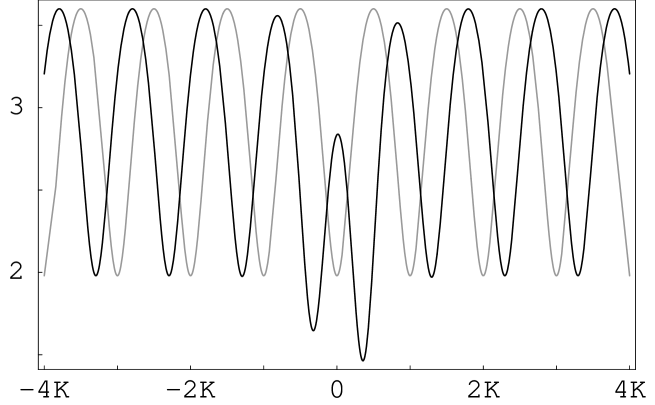
Figure 1: Potential $\widetilde{V}(x)$ with a periodicity defect (black curve) generated from the associated Lamé potential with $m=\ell=1$ (gray curve), $k^{2}=0.99$, and $u(x)=\psi_{1}(x)+3\psi_{2}(x)/2$ with $\epsilon=2.4$, which leads to $a_{1}=-1.089,\ a_{2}=2.607$. The new Hamiltonian $\widetilde{H}$ has an extra bound state at $\epsilon$.

On the other hand, if the seed solution is a linear combination of the two positive definite Bloch functions, $u(x)=\psi_{1}(x)+\lambda\psi_{2}(x)$, then for $\lambda<0$, $u(x)$ will have always a node, inducing then a singular SUSY transformation. For $\lambda=0$ and $\lambda=\infty$ we will recover once again the previously discussed case when $u(x)$ is one of the Bloch functions. Finally, it is interesting to observe that for $\lambda>0$, $u(x)$ will be nodeless, and the new potential will not be strictly periodic (it will have a periodicity defect). The spectrum for the SUSY generated potential $\widetilde{V}(x)$ will consist of the allowed energy bands of the initial potential plus an isolated level embedded in the infinite region below the ‘ground state energy’ of the initial potential. Unfortunately, here the explicit expressions for $\widetilde{V}(x)$ are not compact. Thus, we decided to illustrate this case graphically, and an example of the SUSY partner potential with one periodicity defect of the associated periodic Lamé potential for $m=\ell=1$ is given in Fig. 1 while for $m=2,\ \ell=1$ the corresponding SUSY partner potentials are shown in Fig. 2.

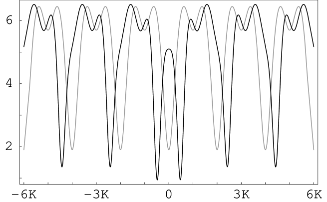
Figure 2: Potential with a periodicity defect (black curve) produced from the associated Lamé potential with $m=2,\ \ell=1$ (gray curve), $k^{2}=0.95$, and $u(x)=\psi_{1}(x)+\psi_{2}(x)$ with $\epsilon=3.5$, which gives $b_{1}=-2.392,\ b_{2}=1.26+0.614\,i,\ b_{3}=b_{2}^{*}$. The new Hamiltonian $\widetilde{H}$ has an extra bound state at $\epsilon$.

4 Conclusions

Through an appropriate ansatz, we have solved the stationary Schrödinger equation for the associated Lamé potentials with an arbitrary energy corresponding to the parameter pairs $(1,1)$ and $(2,1)$. This suggests that the associated Lamé equation with any integer values of the potential parameters is exactly solvable. This assertion can be proved case by case by appropriately modifying the ansatz, given by Eqs. (4),(7) and using a fitting procedure to find the corresponding analytic solution. For instance, one may fit the solution $\Psi(z)=\sum_{r=-2}^{3}C_{r}[\wp(z)-e_{1}]^{r}$ to (3), which will effectively correspond to the point (3,2) in the $m-\ell$ plane, and so on. However, one of the aims of this paper was to show that this can be done through the simplest non-trivial available examples. On the other hand, the first order supersymmetry transformations were used to generate new exactly solvable potentials which can be either periodic or with a periodicity defect, depending on how we choose the seed Schrödinger solutions. This kind of SUSY transformations, together with the second order ones, represent the most simple theoretical tools for designing potentials with prescribed spectra, a subject which every day seems closer to physical reality.

References

- [1] B.K. Bagchi, Supersymmetry in Quantum and Classical Mechanics, Chapman and Hall, Boca Raton, Florida (2000).
- [2] I. Aref’eva, D.J. Fernández, V. Hussin, J. Negro, L.M. Nieto, B.F. Samsonov, Special issue dedicated to the subject of the International Conference on Progress in supersymmetric quantum mechanics, J. Phys. A 37, Number 43 (2004).
- [3] B. Mielnik, O. Rosas-Ortiz, J. Phys. A 37 (2004) 10007.
- [4] J. Negro, L.M. Nieto, O. Rosas-Ortiz, J. Phys. A 37 (2004) 10079.
- [5] A.A. Andrianov, F. Cannata, J. Phys. A 37 (2004) 10297.
- [6] M.V. Ioffe, J. Phys. A 37 (2004) 10363.
- [7] C.V. Sukumar, AIP Conference Proceedings 744 (2005) 166.
- [8] D.J. Fernández, N. Fernández-García, AIP Conference Proceedings 744 (2005) 236 (quant-ph/0502098).
- [9] A. Khare, U. Sukhatme, J. Math. Phys. 40 (1999) 5473.
- [10] A. Ganguly, Mod. Phys. Lett. A 15 (2000) 1923 (math-ph/0204026).
- [11] A. Khare, U. Sukhatme, J. Math. Phys. 42 (2001) 5652.
- [12] A. Ganguly, J. Math. Phys. 43 (2002) 1980 (math-ph/0207028); ibid 43 (2002) 5310 (math-ph/0212045).
- [13] A. Khare, U. Sukhatme, J. Phys. A 37 (2004) 10037.
- [14] E.T. Whittaker, G.N. Watson, A course of modern analysis, Cambridge University Press, Cambridge (1963).
- [15] L. Trlifaj, Inv. Prob. 5 (1989) 1145.
- [16] D.J. Fernández, B. Mielnik, O. Rosas-Ortiz, B.F. Samsonov, J. Phys. A 35 (2002) 4279 (quant-ph/0303051).
- [17] D.J. Fernández, B. Mielnik, O. Rosas-Ortiz, B.F. Samsonov, Phys. Lett. A 294 (2002) 168 (quant-ph/0302204).
- [18] O. Rosas-Ortiz, Rev. Mex. Fís. 49 S2 (2003) 145 (quant-ph/0302189).
- [19] B. Bagchi, A. Ganguly, D. Bhaumik, A. Mitra, Mod. Phys. Lett. A 14 (1999) 27.
- [20] D.J. Fernández, J. Negro, L.M. Nieto, Phys. Lett. A 275 (2000) 338.
- [21] D.J. Fernández, A. Ganguly, in preparation.