Time Optimal Control of Coupled Qubits Under Non-Stationary Interactions

Abstract

In this article, we give a characterization of all the unitary transformations that can be synthesized in a given time for a two-qubit system in the presence of general time varying coupling tensor. This characterization helps to compute the minimum time and the shortest pulse sequence for generating a general two-qubit transformation under non-stationary interactions. The methods presented here can be applied in design of time optimal pulse sequences for transferring coherence and polarization between coupled spins with time varying couplings as in solid state NMR under magic angle spinning.

I Introduction

An important question in quantum information science is to determine the minimum time required to perform a quantum computation using a set of physical resources. Since two-qubit gates are the building blocks of quantum information processing, it is of fundamental interest to find the minimal time required to implement a unitary operation on a two-qubit system using the interaction Hamiltonian $H_{d}$, and the local unitary operations on the two qubits. This problem was studied in Khaneja:01 , where it was shown that any two qubit unitary propogator $U_{F}$ can be expressed as

$$U_{F}=U_{2}\ (\prod_{k=1}^{4}\ V_{k}\exp(-iH_{d}t_{k})\ V_{k}^{\dagger})\ U_{1},$$ (1)

where $U_{1},U_{2},V_{k}$ are local unitary transformations and the effective Hamiltonians $V_{k}H_{d}V_{k}^{\dagger}$ all mutually commute. Under the assumption that the synthesis of local unitaries takes arbitrarily small time, the minimum time to produce a desired $U_{F}$ is the smallest value of $\sum_{k=1}^{4}t_{k}$ in equation (1) Khaneja:01 . This characterization of time optimal trajectories is used in  Vidal to explicitly compute an elegant expression for the minimal time for synthesis of arbitrary unitary transformation of two qubits. Alternate proofs for time optimality have been presented in  Hammerer ; Childs . There is now a considerable literature on the subject; see for example,  Hammerer ; Vidal ; Bullok ; Zhang ; Haselgrove ; Childs ; Zeier ; Vatan ; khanejanmr and references therein.

All these investigations assume that the interaction Hamiltonian $H_{d}$ is fixed. In this paper, we consider the general problem when $H_{d}$ varies with time. For example, in solid state NMR Spiess , the interaction between the spins are varying with time during magic angle spinning when the sample is rotated around an axis making an angle of $\theta_{M}=\tan^{-1}(\sqrt{2})$ with the static magnetic field $B_{0}$. As a result the dipolar couplings between nuclear spins that have an orientational dependence of the form $3\cos^{2}(\theta)-1$ averages out( $\theta$ is the angle of internuclear axis with the static magnetic field), leading to better resolved NMR spectrum Spiess . An important problem in multi-dimensional solid state NMR experiments is to find radio-frequency pulse sequence that re-couple desired spins whose interactions are being modulated in time by magic angle spinning. Finding short pulse sequences that transfer polarization or coherence between coupled nuclear spins under time varying interactions is of interest in solid state NMR. In this paper, we give a complete characterization of all the unitary transformations that can be synthesized in a given time for a two-qubit system in presence of general time varying coupling tensor, assuming that the local unitary transformation on two qubits can be performed arbitrarily fast(on a time scale governed by the strength of couplings). From the perspective of quantum control theory, this problem is equivalent to characterizing the reachable set of the Schr$\ddot{o}$dinger equation

$$\dot{U}(t)=-i[H_{d}(t)+\sum_{j=1}^{m}v_{j}(t)H_{j}]U(t),$$ (2)

where $U\in SU(4)$ and $H_{d}(t)$ is the interaction Hamiltonian that is internal to the system and $\sum_{j=1}^{m}v_{j}(t)H_{j}$ is the part of the Hamiltonian that can be externally changed, and generates the local unitary operations. We assume the control parameters $v_{j}$ are a priori not bounded.

Before stating the main result, we review some background material.

II BACKGROUND

II.1 Majorization

For an element $x=(x_{1},...,x_{k})^{T}$ of $\mathbb{R}^{k}$ we denote by $x^{\downarrow}=(x_{1}^{\downarrow},...,x_{k}^{\downarrow})^{T}$ a permutation of $x$ so that $x_{i}^{\downarrow}\geq x_{j}^{\downarrow}$ if $i<j$, where $1\leq i,j\leq k$.

Definition 1 (majorization)

A vector $x\in\mathbb{R}^{k}$ is majorized by a vector $y\in\mathbb{R}^{K}$ (denoted $x\prec y$), if

$$\sum_{j=1}^{k}x^{\downarrow}_{j}\leq\sum_{j=1}^{k}y^{\downarrow}_{j}$$ (3)

for $k=1,\ldots,D-1$, and the inequality holds with equality when $k=D$.

Proposition 1

$x\prec y$ iff $x$ lies in the convex hull of $y$ and all its permutations $P_{i}y$, where $P_{i}$ are permutation matrices.

Proposition 2 (Schur, Horn  Bhatia ; Horn )

For an element $\lambda=(\lambda_{1},...,\lambda_{n})^{T}$, let $D_{\lambda}$ be a diagonal matrix with $(\lambda_{1},...,\lambda_{n})$ as its diagonal entries, let $a=(a_{1},...,a_{n})^{T}$ be the diagonal entries of matrix $A=K^{T}D_{\lambda}K$, where $K\in SO(n)$. Then $a\prec\lambda$. Conversely for any vector $a\prec\lambda$, there exists a $K\in SO(n)$, such that $(a_{1},...,a_{n})^{T}$ are the diagonal entries of $A=K^{T}D_{\lambda}K$

Following Bennett ; Hammerer ; Vidal , for an element $x=(x_{1},x_{2},x_{3})^{T}$ of $\mathbb{R}^{3}$, we introduce the vector $\hat{x}=(|x_{1}|,|x_{2}|,|x_{3}|)^{T}$, and define the $s$-order version $x^{s}$ of $x$ by setting $x_{1}^{s}=\hat{x}_{1}^{\downarrow}$, $x_{2}^{s}=\hat{x}_{2}^{\downarrow}$, $x_{3}^{s}=sgn(x_{1}x_{2}x_{3})\hat{x}_{3}^{\downarrow}$.

Definition 2 (Bennett ; Hammerer ; Vidal )

The vector $x\in\mathbb{R}^{3}$ is $s$-majorized by $y\in\mathbb{R}^{3}$(denoted $x\prec_{s}y$) if

$$\begin{aligned} x_{1}^{s}&\leq y_{1}^{s}\\ x_{1}^{s}+x_{2}^{s}+x_{3}^{s}&\leq y_{1}^{s}+y_{2}^{s}+y_{3}^{s}\\ x_{1}^{s}+x_{2}^{s}-x_{3}^{s}&\leq y_{1}^{s}+y_{2}^{s}-y_{3}^{s}\end{aligned}$$ (4)

II.2 Canonical Decomposition

An arbitrary two-qubit Hamiltonian can be parameterized

$$H_{d}(t)=I\otimes(\vec{a}(t)\cdot\vec{\sigma})+(\vec{b}(t)\cdot\vec{\sigma})\otimes I+\sum_{i,j}M_{ij}(t)\sigma_{i}\otimes\sigma_{j}$$ (5)

where $i,j\in\{x,y,z\}$ and $\vec{a}\equiv(a_{x},a_{y},a_{z})$, $\vec{b}\equiv(b_{x},b_{y},b_{z})$ are real 3-vectors, $M$ is a 3 by 3 real matrix, and $\vec{\sigma}=(\sigma_{x},\sigma_{y},\sigma_{z})$ is the vector of Pauli operators.

Let $H_{d}^{\prime}(t)$ be the non-local part of $H_{d}(t)$, i.e.,

$$H_{d}^{\prime}(t)=\sum_{i,j}M_{ij}(t)\sigma_{i}\otimes\sigma_{j}.$$

Since we assume that the local unitaries can be generated in arbitrarily small time, all the unitaries transformations that can be synthesized in a given time under $H_{d}(t)$ can also be synthesized under $H_{d}^{\prime}(t)$ and vice versa Khaneja:01 . We therefore consider $H_{d}(t)$ and $H_{d}^{\prime}(t)$ are interchangeable resources under fast local unitaries. From now on we assume $H_{d}(t)$ has only non-local terms.

Proposition 3 (Canonical Decomposition Khaneja:01 ; Kraus )

Any two-qubit non-local Hamiltonian $H$ can be written in the form

$$H=(A\otimes B)^{\dagger}(\theta_{1}^{H}\sigma_{x}\otimes\sigma_{x}+\theta_{2}^{H}\sigma_{y}\otimes\sigma_{y}+\theta_{3}^{H}\sigma_{z}\otimes\sigma_{z})(A\otimes B)$$ (6)

and any two-qubit unitary $U\in SU(4)$ may be written in the form

$$U=(A_{1}\otimes B_{1})e^{-i(\theta_{1}^{U}\sigma_{x}\otimes\sigma_{x}+\theta_{2}^{U}\sigma_{y}\otimes\sigma_{y}+\theta_{3}^{U}Z\otimes Z)}(A_{2}\otimes B_{2})$$ (7)

here $A$, $A_{1}$, $A_{2}$, $B$, $B_{1}$, $B_{2}$ are single-qubit unitaries, and

$$\begin{aligned} \theta_{1}^{H}&\geq\theta_{2}^{H}\geq|\theta_{3}^{H}|\\ \frac{\pi}{4}\geq&\theta_{1}^{U}\geq\theta_{2}^{U}\geq|\theta_{3}^{U}|\end{aligned}$$ (8)

We call $\theta_{1}^{H}\sigma_{x}\otimes\sigma_{x}+\theta_{2}^{H}\sigma_{y}\otimes\sigma_{y}+\theta_{3}^{H}\sigma_{z}\otimes\sigma_{z}$ and $e^{-i(\theta_{1}^{U}\sigma_{x}\otimes\sigma_{x}+\theta_{2}^{U}\sigma_{y}\otimes\sigma_{y}+\theta_{3}^{U}\sigma_{z}\otimes\sigma_{z})}$ the canonical form of $H$ and $U$ respectively, and $\vec{\theta}^{H}$ and $\vec{\theta}^{U}$ the canonical parameters of $H$ and $U$ respectively. For a 3-vector $\vec{\beta}$, we denote

$$H_{\vec{\beta}}=\beta_{1}\sigma_{x}\otimes\sigma_{x}+\beta_{2}\sigma_{y}\otimes\sigma_{y}+\beta_{3}\sigma_{z}\otimes\sigma_{z}$$

$$U_{\vec{\beta}}=e^{-i(\beta_{1}\sigma_{x}\otimes\sigma_{x}+\beta_{2}\sigma_{y}\otimes\sigma_{y}+\beta_{3}\sigma_{z}\otimes\sigma_{z})}$$

II.3 Magic Basis

The magic basis is a vector space basis for two-qubit pure states:

$$\frac{|00\rangle+|11\rangle}{\sqrt{2}}; i\frac{|00\rangle-|11\rangle}{\sqrt{2}};$$

$$i\frac{|01\rangle+|10\rangle}{\sqrt{2}}; \frac{|01\rangle-|10\rangle}{\sqrt{2}}.$$ (9)

The basis change from the standard basis $\{|00\rangle,|01\rangle,|10\rangle,|11\rangle\}$ to the magic basis is given by $Q^{-1}$, where

$$Q=\frac{1}{\sqrt{2}}\left(\begin{array}[]{cccc}1&0&0&i\\ 0&i&1&0\\ 0&i&-1&0\\ 1&0&0&-i\\ \end{array}\right).$$

For elements $U\in SU(4)$ the map $U\rightarrow Q^{-1}UQ$ reflects the isomorphism between $SU(2)\otimes SU(2)$ and $SO(4)$ Makhlin . When expressed in the magic basis, canonical form Hamiltonian and unitaries are diagonal. In magic basis, the canonical decomposition takes the form $H_{d}=K^{T}D_{H}K$, $U=RD_{U}S$, where $K$, $R$ and $S$ are real orthogonal matrices, and $D_{H}$, $D_{U}$ are diagonal matrices. The diagonal elements of $D_{H}$ and $D_{U}$ are easily written in the terms of the canonical form parameters $\theta^{i},i\in\{H,U\}$. Define

$$\begin{aligned} \varphi_{1}^{i}&=\theta_{1}^{i}+\theta_{2}^{i}-\theta_{3}^{i},\varphi_{2}^{i}=\theta_{1}^{i}-\theta_{2}^{i}+\theta_{3}^{i},\\ \varphi_{3}^{i}&=-\theta_{1}^{i}+\theta_{2}^{i}+\theta_{3}^{i},\varphi_{4}^{i}=-\theta_{1}^{i}-\theta_{2}^{i}-\theta_{3}^{i}.\end{aligned}$$ (10)

The diagonal elements of $D_{H}$ are $(\varphi_{1}^{H},\varphi_{2}^{H},\varphi_{3}^{H},\varphi_{4}^{H})$ and the diagonal elements of $D_{U}$ are $(e^{-i\varphi_{1}^{U}},e^{-i\varphi_{2}^{U}},e^{-i\varphi_{3}^{U}},e^{-i\varphi_{4}^{U}})$. Under choice of magic basis, $H_{d}$ is real symmetric and $(\varphi_{1}^{H},\varphi_{2}^{H},\varphi_{3}^{H},\varphi_{4}^{H})$ are its eigenvalues. Eq.(8) together with Eq.(10) implies that

$$\varphi_{1}^{i}\geq\varphi_{2}^{i}\geq\varphi_{3}^{i}\geq\varphi_{4}^{i}.$$

Proposition 4 (Hammerer )

Let $\vec{\alpha}$ and $\vec{\beta}$ be two real s-ordered 3-vectors, let $\vec{\lambda}$ and $\vec{\mu}$ be the 4-vectors related to $\vec{\alpha}$ and $\vec{\beta}$ respectively via (10), then $\vec{\lambda}\prec\vec{\mu}$ iff $\vec{\alpha}\prec_{s}\vec{\beta}$.

The proof follows from the definitions.

III Result

The main result of this paper is as follows:

Theorem 1

Let $\vec{\theta}^{H}(t)$ be the canonical parameters of $H_{d}(t)$ in (2) and $\vec{\theta}(T)=\int_{0}^{T}\theta^{H}(t)\mathrm{d}t$, where the integration is performed for each entry of the vector. All the unitary operators that can be generated within time T with $H_{d}(t)$ and fast local unitaries are given by the set

$${\cal{R}}(T)=\{K_{1}U_{\vec{\beta}}K_{2}|K_{1},K_{2}\in SU(2)\otimes SU(2),\vec{\beta}\prec_{s}\vec{\theta}(T)\}$$

Remark 1

We prove this theorem by using the choice of magic basis. In this basis, $\{-iH_{j}\}$ are skew-symmetric matrices and generate the group $SO(4)$. The interaction Hamiltonian $H_{d}$ can be expressed as $H_{d}=K^{T}D_{\vec{\lambda}}K$, where $K\in SO(4)$ and $D_{\vec{\lambda}}$ a diagonal matrix with diagonal entry $\vec{\lambda}$ related to $\vec{\theta}^{H}$ via (10). Let $\vec{\gamma}(T)=\int_{0}^{T}\vec{\lambda}(t)\mathrm{d}t$, then in the magic basis

$${\cal{R}}(T)=\{Re^{-iD_{\vec{\beta}}}S|R,S\in SO(4),\vec{\beta}\prec\vec{\gamma}(T)\}.$$

Proof: Under the choice of magic basis, we can write $U(t)=R(t)A(t)S(t)$, where $R(t),S(t)\in SO(4)$ and $A(t)$ be diagonal matrix. Assumption of fast local unitaries implies we can generate $SO(4)$ instantly , so it suffices to prove all we can generate for the $A$ part is $e^{-iD_{\vec{\beta}}}$, $\vec{\beta}\prec\vec{\gamma}(T)$.

Assume $U(t)=R(t)A(t)S(t)$ is a trajectory of Eq.(2), then $A(t)=R^{T}(t)U(t)S^{T}(t)$ and $\dot{A}(t)=$

$$\dot{R}^{T}(t)U(t)S^{T}(t)+R^{T}(t)\dot{U}(t)S^{T}(t)+R^{T}(t)U(t)\dot{S}^{T}(t).$$

Let $\dot{R}^{T}(t)=r(t){R}^{T}(t)$ and $\dot{S}^{T}(t)={S}^{T}(t)s(t)$, substituting for $\dot{U}(t)$, we get $R^{T}(t)\dot{U}(t)S^{T}(t)=$

$$R^{T}(t)\ [-iH_{d}(t)\\ -i\sum_{i=1}^{m}v_{j}(t)H_{j}]R(t)(R^{T}(t)U(t)S^{T}(t)).$$

Using $H_{d}(t)=K^{T}(t)D_{\vec{\lambda}}K(t)$ we get $R^{T}(t)\dot{U}(t)S^{T}(t)=$

$$R^{T}(t)\ [-iK^{T}(t)D_{\vec{\lambda}}K(t)\\ -i\sum_{i=1}^{m}v_{j}(t)H_{j}]R(t)(A(t)).$$

Let $P(t)=K(t)R(t)$ and denote $h(t)=R^{T}(t)\ [-i\sum_{i=1}^{m}v_{j}(t)H_{j}]R(t)$. Equation for evolution of $A(t)$ then takes the form $\dot{A}(t)=$

$$r(t)A(t)+[P^{T}(t)D_{\vec{\lambda}}(t)P(t)]A(t)+h(t)A(t)+A(t)s(t).$$ (11)

Notice that $r(t),s(t)$, and $h(t)$ are in $so(4)$ (skew symmetric matrices of dimension 4) and hence their diagonal entries are all zero. When multiplied by a diagonal matrix $A(t)$, the diagonal entries remain zero. Therefore in the evolution equation of $A(t)$, these terms must sum to zero and we can discard these terms. We get

$$\dot{A}(t)=D_{-i\vec{\mu}(t)}A(t)$$ (12)

where $\vec{\mu}(t)$ is the diagonal entries of $P^{T}(t)D_{\vec{\lambda}(t)}P(t)$. Since we can generate elements of $SO(4)$ in arbitrarily small time, $R(t)$ and hence $P(t)$ can take value of any element in $SO(4)$ and from Proposition (2), $\vec{\mu}(t)$ can take any element of the set $\{\vec{\mu}(t)|\vec{\mu}(t)\prec\vec{\lambda}(t)\}$.

From Eq.(12), we get $A(T)=e^{-iD_{\vec{\beta}}}$, where $\vec{\beta}=\int_{0}^{T}\vec{\mu}(t)\mathrm{d}t$, $\vec{\mu}(t)\prec\vec{\lambda}(t)$. We first prove $\vec{\beta}\prec\vec{\gamma}(T)$, and then show that $\vec{\beta}$ can take on the values of any vector majorized by $\vec{\gamma}(T)$.

$$\sum_{j=1}^{k}\gamma^{\downarrow}_{j}(T)=\sum_{j=1}^{k}\int_{0}^{T}\lambda^{\downarrow}_{j}(t)\mathrm{d}t$$ (13)

$$\sum_{j=1}^{k}\beta^{\downarrow}_{j}=\sum_{j=1}^{k}\int_{0}^{T}\mu_{\sigma(j)}(t)\mathrm{d}t$$ (14)

where $\sigma$ is some permutations and $k=1,2,3,4$. On subtracting Eq.(14) from Eq.(13), we get

$$\begin{aligned} \sum_{j=1}^{k}\gamma^{\downarrow}_{j}(T)-\sum_{j=1}^{k}\beta^{\downarrow}_{j}=\int_{0}^{T}\sum_{j=1}^{k}\lambda^{\downarrow}_{j}(t)-\sum_{j=1}^{k}\mu_{\sigma(j)}(t)\mathrm{d}t.\end{aligned}$$ (15)

Since $\mu(t)\prec\lambda(t)$, $\sum_{j=1}^{k}\lambda^{\downarrow}_{j}(t)-\sum_{j=1}^{k}\mu_{\sigma(j)}(t)\geq 0$, and from Eq.(15), $\sum_{j=1}^{k}\gamma^{\downarrow}_{j}(T)-\sum_{j=1}^{k}\beta^{\downarrow}_{j}\geq 0$. Obviously when $k=4$, both terms equal 0, the equality holds, so $\vec{\beta}\prec\vec{\gamma}(T)$.

We now prove $\vec{\beta}$ can take on the values of all the vectors majorized by $\vec{\gamma}(T)$, which is the convex hull of $\vec{\gamma}(T)$ and all its permutations. If we take $R(t)=K^{T}(t)$, then $\vec{\beta}=\vec{\gamma}(T)$. It is also easy to see $\vec{\beta}$ can take all the permutations of $\vec{\gamma}(T)$, so we just need to prove that the vectors $\vec{\beta}$ can reach is a convex set. Let $\alpha\in[0,1]$,

$$\vec{\beta}_{1}=\int_{0}^{T}\vec{\mu}_{1}(t)\mathrm{d}t$$ (16)

$$\vec{\beta}_{2}=\int_{0}^{T}\vec{\mu}_{2}(t)\mathrm{d}t$$ (17)

then

$$\alpha\vec{\beta}_{1}+(1-\alpha)\vec{\beta}_{1}=\int_{0}^{T}\alpha\vec{\mu}_{1}(t)+(1-\alpha)\vec{\mu}_{2}(t)\mathrm{d}t$$ (18)

but $\alpha\vec{\mu}_{1}(t)+(1-\alpha)\vec{\mu}_{2}(t)\prec\vec{\lambda}(t)$, so $\alpha\vec{\beta}_{1}+(1-\alpha)\vec{\beta}_{1}$ can also be achieved. Q.E.D

Given these theorems, we can compute the minimum time needed to generate any unitary operator $U$ in $SU(4)$ with $H_{d}(t)$ and fast local unitaries.

Theorem 2

Using the Hamiltonian $H_{d}(t)$ and fast local unitaries, a two-qubit gate $U$ can be generated within time T iff there exists a vector $\vec{n}=(n_{1},n_{2},n_{3})$ of integers, such that $\vec{\beta}_{\vec{n}}=\vec{\theta}^{\ U}+\frac{\pi}{2}\vec{n}$ satisfies

$$\vec{\beta}_{\vec{n}}\prec_{s}\int_{0}^{T}\vec{\theta}^{H_{d}(t)}\mathrm{d}t$$

where $\vec{\theta}^{\ U}$ and $\vec{\theta}^{H_{d}(t)}$ are the canonical parameters of $U$ and $H_{d}(t)$ respectively. The minimum time required to simulate $U$ is given by the minimum value of $T\geq 0$ such that either

$$\vec{\beta}_{(0,0,0)}\prec_{s}\int_{0}^{T}\vec{\theta}^{H_{d}(t)}\mathrm{d}t$$ (19)

or

$$\vec{\beta}_{(-1,0,0)}\prec_{s}\int_{0}^{T}\vec{\theta}^{H_{d}(t)}\mathrm{d}t$$ (20)

holds

The proof follows the treatment in  Vidal .

Proof: Recall that all commutators $[\sigma_{j}\otimes\sigma_{j},\sigma_{k}\otimes\sigma_{k}]$ vanish, and that $\exp(-i\frac{\pi}{2}\sigma_{j}\otimes\sigma_{j})=-i\sigma_{j}\otimes\sigma_{j}$ is a local gate. This implies that $\vec{\theta}^{\ U}+\frac{\pi}{2}\vec{n}$ represents all vectors compatible with the gate $U$. It is straightforward to check from Eq.(4) that for any two vectors $\vec{x}$ and $\vec{y}$, with components $x_{1}\geq x_{2}\geq|x_{3}|$, $y_{1}\geq y_{2}\geq|y_{3}|$, if $y_{1}\geq 3x_{1}$, then $\vec{x}\prec_{s}\vec{y}$. By definition $\frac{\pi}{4}\geq\theta^{U}_{1}\geq 0$, if some component $n_{j}$ of $\vec{n}$ fulfills $|n_{j}|>1$, then the maximal component of the reordered version of $\vec{\theta}^{\ U}+\frac{\pi}{2}\vec{n}$ is at least $\frac{3\pi}{4}$, which implies $\vec{\theta}^{\ U}\prec_{s}\vec{\theta}^{U}+\frac{\pi}{2}\vec{n}$. Therefore we can restrict our attention to vectors $\vec{n}$ with $|n_{j}|\leq 1$. A case by case check shows that for $\vec{n}\in\{(-1,-1,-1),(0,-1,0),(0,0,-1),(0,0,1)\}$, $\vec{\theta}^{\ U}+\frac{\pi}{2}(-1,0,0)\prec_{s}\vec{\theta}^{\ U}+\frac{\pi}{2}\vec{n}$, and for the remaining vectors $\vec{n}$, $\vec{\theta}^{\ U}+\frac{\pi}{2}(0,0,0)\prec_{s}\vec{\theta}^{\ U}+\frac{\pi}{2}\vec{n}$. Thus the result follows.

IV Example

We now work an explicit example on finding the minimum time to synthesize a desired unitary under time varying couplings. Assume the interaction $H_{d}(t)$ takes the form $D(t)(\sigma_{x}\otimes\sigma_{x}+\sigma_{y}\otimes\sigma_{y}-2\sigma_{z}\otimes\sigma_{z})$. We compute the minimum time to generate a swap gate corresponding to the unitary transformation $U=\exp{-i\frac{\pi}{4}(\sigma_{x}\otimes\sigma_{x}+\sigma_{y}\otimes\sigma_{y}+\sigma_{z}\otimes\sigma_{z})}$.

To fix ideas, consider the case when $D(t)$ is constant, say $D>0$. The canonical parameters of $H_{d}(t)$ and $U$ are $D(2,1,-1)$ and $\frac{\pi}{4}(1,1,1)$ respectively. The minimum time to generate $U$ is the minimum $T$ that satisfies $\frac{\pi}{4}(1,1,1)\prec_{s}DT(2,1,-1)$ or $\frac{\pi}{4}(1,1,1)+\frac{\pi}{2}(-1,0,0)\prec_{s}DT(2,1,-1)$, which is $\frac{3\pi}{16D}$. The strategy to generate $U$ is to use selective excitation on first spin preparing an effective Hamiltonian $D(-\sigma_{x}\otimes\sigma_{x}+\sigma_{y}\otimes\sigma_{y}+2\sigma_{z}\otimes\sigma_{z})$, which evolves $\frac{\pi}{16D}$ units of time. This is followed by evolution of effective Hamiltonians $D(-2\sigma_{x}\otimes\sigma_{x}+\sigma_{y}\otimes\sigma_{y}+\sigma_{z}\otimes\sigma_{z})$ and $D(-\sigma_{x}\otimes\sigma_{x}+2\sigma_{y}\otimes\sigma_{y}+\sigma_{z}\otimes\sigma_{z})$ for $\frac{\pi}{16D}$ units of time each. In the end we apply a local unitaries $e^{-i\frac{\pi}{2}\sigma_{x}\otimes\sigma_{x}}=-i\sigma_{x}\otimes\sigma_{x}$.

Now consider the time-dependent case, which models the variation of coupling strength between homo-nuclear spins under magic angle spinning Spiess . The dipolar interaction strength $D(t)$ during magic angle spinning varies in time as $D(t)=D\frac{3\cos^{2}(\theta(t))-1}{2}$, where $\theta(t)$ is the angle internuclear vector makes with the $B_{0}$ field. The angle $\theta(t)$ changes as the sample is being rotated around an axis making an angle $\theta_{M}=\tan^{-1}(\sqrt{2})$ with the $B_{0}$ field. Let $\beta$ denote the angle internuclear axis makes with the magic angle axis. Then we can express $\theta(t)$ as

$$\cos(\theta(t))=\cos(\beta)\cos(\theta_{M})+\sin(\beta)\cos(\omega t)\sin(\theta_{M}),$$

where $\omega$ is the spinning frequency. $D(t)$ is then a periodic function. We choose $\beta=\frac{\pi}{4}$ and plot modulation of $D(t)$ in figure  1. Each period of $D(t)$ can be divided into two parts, $\{D(t)\leq 0\}\bigcup\{D(t)>0\}$. Let $S_{1}$, $S_{2}$ denote the area of these two parts respectively, i.e., $S_{1}=-\int_{\{D(t)\leq 0\}}D(t)\mathrm{d}t$, $S_{2}=\int_{\{D(t)>0\}}D(t)\mathrm{d}t$. We find that $S_{1}=S_{2}=\frac{1.4922}{\omega}D$.

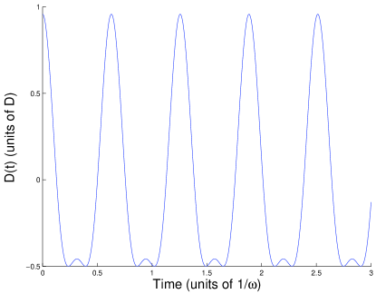
Figure 1: The figure shows the modulation of the coupling strength $D(t)$ as function of time for $\beta=\frac{\pi}{4}$

The canonical parameters for $H_{d}(t)$ are

$$\left\{\begin{array}[]{ll}D(t)(2,1,-1)&\textrm{for }D(t)\geq 0\\ -D(t)(2,1,1)&\textrm{for }D(t)<0\\ \end{array}\right.$$

i.e., $(2|D(t)|,|D(t)|,-D(t))$. Using theorem (2), we get the minimum time to generate $U$ is the smallest $T$ that satisfies

$$\frac{3\pi}{4}\leq\int_{0}^{T}3|D(t)|-D(t)\mathrm{d}t$$

when $\omega>>D$, $\int_{0}^{T}3|D(t)|-D(t)\mathrm{d}t$ is approximately $n(2S_{1}+4S_{2})$, where $n$ is the number of periods of $D(t)$ within time T, so the minimum $n=\lceil\frac{3\pi}{4(2S_{1}+4S_{2})}\rceil=\lceil\frac{0.2632\omega}{D}\rceil$ and the minimum time $T$ is approximately $2\pi\frac{n}{\omega}$. The pulse sequence prepares effective Hamiltonians $(-\sigma_{x}\otimes\sigma_{x}+\sigma_{y}\otimes\sigma_{y}+2\sigma_{z}\otimes\sigma_{z})$, $(-2\sigma_{x}\otimes\sigma_{x}+\sigma_{y}\otimes\sigma_{y}+\sigma_{z}\otimes\sigma_{z})$ and $(-\sigma_{x}\otimes\sigma_{x}+2\sigma_{y}\otimes\sigma_{y}+\sigma_{z}\otimes\sigma_{z})$ for $n/3$ periods each, in the part of the period when $D(t)>0$. Similarly, we prepare effective Hamiltonians $(-\sigma_{x}\otimes\sigma_{x}-\sigma_{y}\otimes\sigma_{y}+2\sigma_{z}\otimes\sigma_{z})$, $(\sigma_{x}\otimes\sigma_{x}+2\sigma_{y}\otimes\sigma_{y}-\sigma_{z}\otimes\sigma_{z})$ and $(-2\sigma_{x}\otimes\sigma_{x}+\sigma_{y}\otimes\sigma_{y}+\sigma_{z}\otimes\sigma_{z})$ for $n/3$ periods each, in the part of the period when $D(t)<0$. As before, we apply a local rotation $e^{-i\frac{\pi}{2}\sigma_{x}\otimes\sigma_{x}}$ in the end.

V Conclusion

In this paper, we studied the problem of time-optimal synthesis of a unitary transformation for coupled qubits under non-stationary interactions. Under the assumption that local unitary transformations can be synthesized arbitrarily fast, we characterized the time optimal trajectories and the minimal time to prepare a general two qubit rotation under general time varying coupling tensor. These results generalize the results presented in  Khaneja:01 ; Hammerer ; Vidal for stationary coupling Hamiltonians to the non-stationary case. The problem considered in this paper was motivated by design of time optimal pulse sequences for controlling coupled spin dynamics in solid state NMR spectroscopy, where couplings between spins are modulated in time due to magic angle spinning. The results presented here are of fundamental interest and may find applications in some implementations of quantum information processing.

References

• (1) R.Bhatia, ”Matrix Analysis” Springer-Verlag, New York, 1997.
• (2) A.Horn, β€œDoubly stochastic matrices and the diagonal of a rotation matrix” Amer.J.Math, vol. 76 p.620-630, 1954.
• (3) N.Khaneja, R.Brockett and S.J.Glaser, Phys. Rev. A 63, 032308(2001).
• (4) B. Kraus and J.I. Cirac, Phys. Rev. A 63, 062309(2001).
• (5) C.H.Bennett, J.I.Cirac, M.S.Leifer, D.W.Leung, N.Linden, S.Popescu and G.Vidal, Phys. Rev. A 66, 012305(2002).
• (6) G. Vidal, K. Hammerer, and J. I. Cirac, Phys. Rev. Lett. 88, 237902(2002).
• (7) K. Hammerer, G. Vidal, and J. I. Cirac, Phys. Rev. A 66, 062321(2002).
• (8) S.S.Bullock and I.L.Markov, Phys. Rev. A 68, 012318(2003).
• (9) J.Zhang, J.Vala, S.Sastry, and K.B.Whaley, Phys. Rev. Lett. 91, 027903(2003).
• (10) H.L.Haselgrove, M.A.Nielsen, and T.J.Osborne, Phys. Rev. A 68, 042303(2003).
• (11) A.M.Childs, H.L.Haselgrove, and M.A.Nielsen, Phys. Rev. A 68, 052311(2003).
• (12) R.Zeier, M.Grassl, and T.Beth, Phys. Rev. A 70, 032319(2004).
• (13) F.Vatan and C.Williams, Phys. Rev. A 69, 032315(2004).
• (14) N. Khaneja, F. Kramer, S.J. Glaser, J. Magn. Reson. 173, 116-124 (2005).
• (15) C.D.Hill and H.-S.Goan, Phys. Rev. A 68, 012321(2003).
• (16) Y.Makhlin, Quantum Inf. Process. 1, 243(2002).
• (17) Klaus Schmidt-Rohr and Hans Wolfgang Spiess, Multidimensional Solid-State NMR and Polymers (Academic Press) (1994).