Fault-Tolerant Dissipative Preparation of Atomic Quantum Registers with Fermions

Abstract

We propose a fault tolerant loading scheme to produce an array of fermions in an optical lattice of the high fidelity required for applications in quantum information processing and the modelling of strongly correlated systems. A cold reservoir of Fermions plays a dual role as a source of atoms to be loaded into the lattice via a Raman process and as a heat bath for sympathetic cooling of lattice atoms. Atoms are initially transferred into an excited motional state in each lattice site, and then decay to the motional ground state, creating particle-hole pairs in the reservoir. Atoms transferred into the ground motional level are no longer coupled back to the reservoir, and doubly occupied sites in the motional ground state are prevented by Pauli blocking. This scheme has strong conceptual connections with optical pumping, and can be extended to load high-fidelity patterns of atoms.

I Introduction

High-precision control of cold atoms in optical lattices has found many potential applications in recent years, especially in the implementation of quantum information processing and the modelling of strongly correlated condensed matter systems hubbardtoolbox . These applications have been fuelled by experimental techniques which enable engineering of lattice models with sensitive control over lattice parameters Greiner ; Esslinger1D ; Paredes1D , independent control for different internal spin states sdol , and control of interactions between atoms via Feshbach resonances magfeshbach ; optfeshbach .

For high precision applications, initial state preparation will play a key role in addition to such control of Hamiltonian parameters Paeda . Quantum computing applications generally require an initial register with exactly one atom per lattice site Deutschreview , and observation of interesting effects in strongly correlated systems often requires the initial spatial patterns of atoms or states with precisely chosen filling factors LewensteinKagome .

The first step in preparation of such states is often adiabatically increasing the lattice potential, making use of repulsive onsite interactions for bosons jaksch98 or Pauli blocking for fermions Calarcoloading to load essentially one atom on each lattice site. However, experimental imperfections will generally lead to non-negligible errors in the resulting states. This can be improved upon by coherently filtering a state with a filling factor initially greater than one Paeda ; CiracEnsemble , or potentially by schemes involving individual addressing and precise measurement of the occupation in individual lattice sites BrennenRegister ; WeissLoading . Whilst these methods can, in principle, produce high fidelity initial states, each of them relies either on the perfect experimental implementation of a single-shot coherent process or on perfect measurements to avoid defects in the final state. In this article we propose a fault-tolerant loading scheme in which the state being prepared always improves in time. The key idea is the addition of a dissipative element to the loading process, in contrast to previous schemes, which rely on coherent transfer or perfect measurements. As we will see below, this dissipative element plays a similar role in our scheme to that of spontaneous emissions in optical pumping.

Motivated by advances in experiments with cold fermions Jin99 ; Grimm03 ; Jin03a ; Ketterle04 ; Inguscio02 ; Esslinger3D ; Salomon04 ; Hulet03 ; Thomas04 , our scheme is designed to produce a regular patterned array of fermions in an optical lattice. Fermions have a natural advantage in initialising atomic qubit registers because Pauli-blocking prevents doubly-occupied sites, and most of the techniques illustrated using bosons in quantum computing proposals apply equally to fermions. Fermionic species are also of special interest in the simulation of condensed matter systems HofstetterFermiLattice .

Figure 1: Laser-assisted dissipative loading of fermions in an optical lattice: (a) Atoms are coupled from an external reservoir (in internal state $|b\rangle$) into an excited motional state in the lattice (internal state $|a\rangle$ via a Raman process; (b) These atoms are cooled to the ground motional level via collisional interaction with the reservoir atoms, and doubly-occupied sites in the ground level are prevented by Pauli blocking; (c) Remaining atoms in the excited motional levels are removed by carefully detuning the Raman coupling above the Fermi Energy.

The setup for our scheme is illustrated in Fig. 1. Atoms in an internal state $|b\rangle$ do not couple to the lattice lasers, and form a cold Fermi reservoir, which will play the dual role of a source for atoms to transfer into the lattice, and a bath for cooling lattice atoms. Atoms in the reservoir are coupled into an excited motional level in the lattice (in internal state $|a\rangle$) via a coherent laser-induced Raman process (Fig. 1a) Raizen04 . These atoms are then cooled sympathetically by the reservoir atoms via collisional interactions, and will decay to the motional ground state together with creation of a particle-hole pair in the reservoir (Fig. 1b). This is analogous to the sympathetic cooling process previously presented for a bosonic reservoir in AJ . Double occupancy in the ground state is prevented by Pauli blocking (Fig. 1b), and atoms in the ground state are not coupled back to the reservoir because the Raman process is far off resonance, so the occupation of the lowest motional level always increases in time. Additional atoms remaining in excited states at the end of the process can then be removed by a careful adiabatic detuning and switching off of the coupling lasers (Fig. 1c).

Such dissipative transfer of atoms into a desired dark state is strongly reminiscent of optical pumping, in which atoms are excited by a laser, and undergo spontaneous emissions into a desired state which does not couple to the laser field. The net result of this is to transfer entropy from the atomic system into the “reservoir” (the vacuum modes of the radiation field) in order to produce a single pure electronic state from an initial mixed state. Here the creation of an excitation in the reservoir replaces the spontaneous emission event, placing the atom in a state where it is not coupled by the Raman process, and leading to the production of our final pure state, namely a high fidelity array of one atom in each lattice site (or a pattern of occupied and unoccupied sites).

We note, in addition, that the purely coherent laser-assisted loading could be used as a stand-alone technique to load the lattice, and could produce high fidelity states if used iteratively, together with cooling of the Fermi reservoir. Such cooling would fill holes produced in the previous loading step, so that Pauli blocking would prevent a net transfer of atoms from the lattice to the reservoir, thus ensuring that the filling factor in the lattice is improved in each step.

The detailed analysis of this dissipative loading process is divided into two parts. Coherent laser-assisted loading of atoms into the entire lattice in a single addressed motional band is discussed in section II, and the dissipative transfer of atoms to the lowest motional band is analysed in section III. The combination of these two elements into the overall scheme is then detailed in section IV.

II Laser-Assisted Loading

We begin by studying the coupling of the atoms forming the reservoir into the optical lattice via a Raman process, as shown in Fig. 1. The atoms in the Reservoir are in an internal state $|b\rangle$, which does not couple to the lasers producing the optical lattice. They form a Fermi gas containing $N$ atoms with a density $n_{3\rm D}=N/V$ in a volume $V$, with Fermi energy ($\hbar=1$) $\epsilon_{F}=\left(6\pi^{2}n_{3\rm D}\right)^{2/3}/2m$, where $m$ is the mass of the atoms. The internal state $|b\rangle$ is coupled to a different internal state $|a\rangle$, which is trapped by a deep three dimensional optical lattice potential $V_{a}({\mathbf{x}})$ via a Raman transition.

Our goal is to couple atoms $b$ into the lattice and to achieve an average occupation of fermions close to one in all lattice sites in one chosen motional band, without coupling to other motional levels. This should be achieved in a time, where no atoms are allowed to tunnel between different lattice sites and no loss of atoms occurs (due to, e.g., spontaneous emission events leading to additional internal states etc.).

II.1 The Model

The total Hamiltonian of this system is given by

$$H=H_{a}+H_{b}+H_{\rm RC},$$ (1)

where the Hamiltonians for the atoms $a$ in the optical lattice and for the atoms $b$ forming the reservoir are

$$H_{a}=\int{\rm d}^{3}x\hat{\psi}_{a}^{\dagger}({\mathbf{x}})\left(-\frac{\nabla^{2}}{2m}+V_{a}({\mathbf{x}})\right)\hat{\psi}_{a}({\mathbf{x}}),$$ (2)

and

$$H_{b}=\int{\rm d}^{3}x\hat{\psi}_{b}^{\dagger}({\mathbf{x}})\left(-\frac{\nabla^{2}}{2m}\right)\hat{\psi}_{b}({\mathbf{x}}),$$ (3)

respectively, in which the anticommuting field operators $\hat{\psi}_{i}^{\dagger}({\mathbf{x}})$ create a fermion in the internal state $i\in\{a,b\}$ at the position ${\mathbf{x}}$.

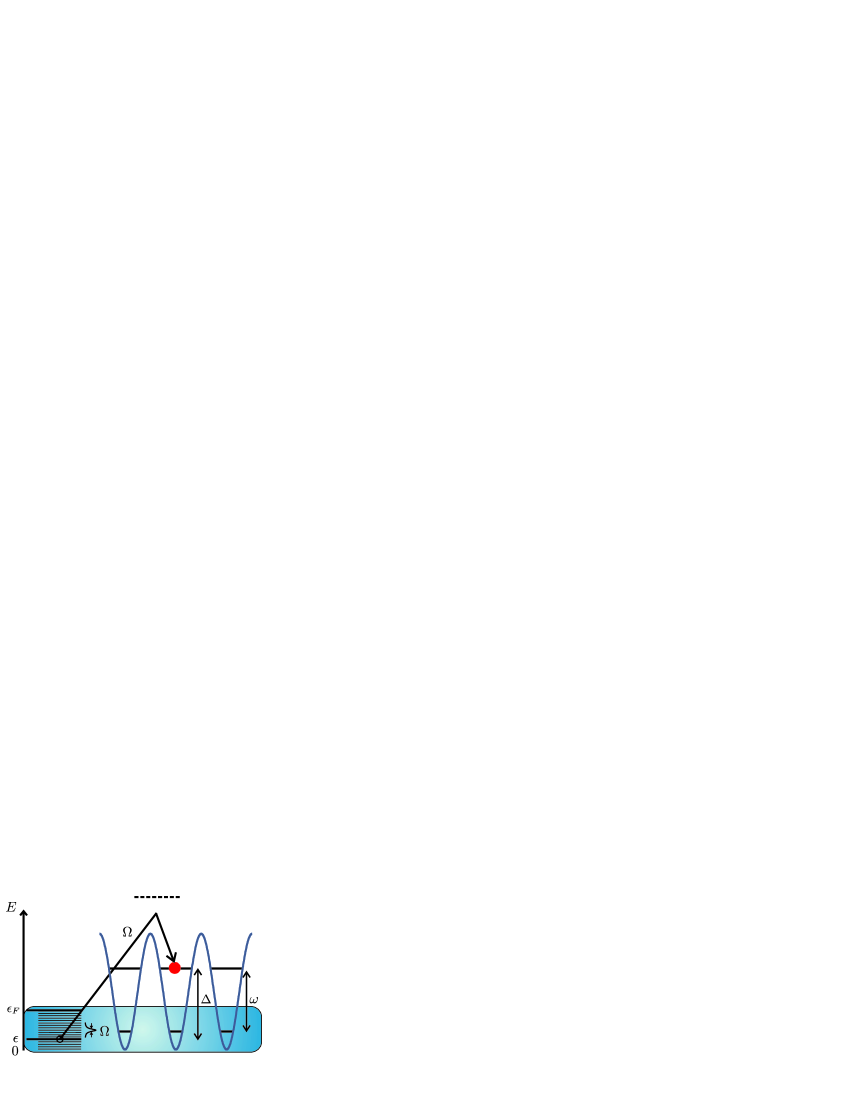
Figure 2: Reservoir atoms with energy $\epsilon$ are resonantly coupled to the first excited Bloch band of the lattice via a Raman laser with two photon Rabi frequency $\Omega$. The resonant energy $\epsilon$ is experimentally tunable via the Raman detuning, and the energy separation of the two Bloch bands is denoted by $\omega$.

The two internal states are coupled via a Raman process described by the Hamiltonian

$$H_{\rm RC}=\int{\rm d}^{3}x \left[\frac{\Omega}{2}\left(\hat{\psi}_{b}^{\dagger}({\mathbf{x}})\hat{\psi}_{a}({\mathbf{x}})+{\rm h.c.}\right)\right.$$

$$\left.\quad+\Delta\hat{\psi}_{a}^{\dagger}({\mathbf{x}})\hat{\psi}_{a}({\mathbf{x}})\right],$$ (4)

with the Raman detuning $\Delta$ and the effective (two photon) Rabi frequency $\Omega$, where we have assumed running waves with the same wave vectors for two lasers producing the Raman coupling.

We expand the field operators for the free fermions in the reservoir as plane waves and the field operators for the lattice atoms in terms of Wannier functions,

$$\hat{\psi}_{b}({\mathbf{x}})=\frac{1}{\sqrt{V}}\sum_{\mathbf{k}}{\rm e}^{{\rm i}{\mathbf{k}}{\mathbf{x}}}b_{\mathbf{k}},$$

$$\hat{\psi}_{a}({\mathbf{x}})=\sum_{\alpha,{\mathbf{n}}}w_{\mathbf{n}}({\mathbf{x}}-{\mathbf{x}}_{\alpha})a_{\alpha,{\mathbf{n}}},$$ (5)

where, $b_{\mathbf{k}}^{\dagger}$ creates a reservoir atom with momentum ${\mathbf{k}}$, $a_{\alpha,{\mathbf{n}}}^{\dagger}$ is the creation operator for an atom in lattice site $\alpha$ and motional state with ${\mathbf{n}}=(n_{x},n_{y},n_{z})$ in the deep three dimensional optical lattice, for which $w_{\mathbf{n}}({\mathbf{x}}-{\mathbf{x}}_{\alpha})$, denotes the corresponding Wannier function.

Inserting into Eqs. (2)-(II.1) we obtain

$$H_{b}=\sum_{\mathbf{k}}\epsilon_{\mathbf{k}}b_{\mathbf{k}}^{\dagger}b_{\mathbf{k}},$$

$$H_{a}=\sum_{\alpha,{\mathbf{n}}}\left(\omega_{\mathbf{n}}+\Delta\right)a_{\alpha,{\mathbf{n}}}^{\dagger}a_{\alpha,{\mathbf{n}}},$$

$$H_{\rm RC}=\frac{\Omega}{2}\sum_{{\mathbf{k}},\alpha,{\mathbf{n}}}\left(R_{{\mathbf{k}},{\mathbf{n}}}{\rm e}^{-{\rm i}{\mathbf{k}}{\mathbf{x}}_{\alpha}}b_{\mathbf{k}}^{\dagger}a_{\alpha,{\mathbf{n}}}+{\rm h.c.}\right),$$ (6)

where the single particle energy of a reservoir atom with momentum ${\mathbf{k}}$ is $\epsilon_{\mathbf{k}}=|{\mathbf{k}}|^{2}/2m$ and the energy of a lattice atom in the motional state ${\mathbf{n}}$ is given by

$$\omega_{\mathbf{n}}=\int{\rm d}^{3}xw_{\mathbf{n}}({\mathbf{x}})\left(-\frac{\nabla^{2}}{2m}+V_{a}({\mathbf{x}})\right)w_{\mathbf{n}}({\mathbf{x}}).$$ (7)

As we are dealing with very deep optical lattices, tunneling between different lattices sites is strongly suppressed and has thus been neglected. The Raman coupling parameter $R_{{\mathbf{k}},{\mathbf{n}}}$ can be written as

$$R_{{\mathbf{k}},{\mathbf{n}}}=\frac{1}{\sqrt{V}}\int{\rm d}^{3}x{\rm e}^{-{\rm i}{\mathbf{k}}{\mathbf{x}}}w_{\mathbf{n}}({\mathbf{x}}).$$ (8)

For our deep optical lattices without tunneling between different sites, the periodic lattice is equivalent to an array of independent microtraps, where each individual trap is well approximated by a harmonic oscillator. The Wannier functions $w_{\mathbf{n}}({\mathbf{x}}-{\mathbf{x}}_{\alpha})$ can then be approximated by harmonic oscillator eigenfunctions $\phi_{\mathbf{n}}({\mathbf{x}}-{\mathbf{x}}_{\alpha})$ of the ${\mathbf{n}}$-th oscillator level in lattice site $\alpha$. This approximation allows us to calculate the coupling parameters $R_{{\mathbf{k}},{\mathbf{n}}}$ from the Fermi reservoir to the optical lattice explicitly. For an isotropic three dimensional lattice (where the frequency $\omega$ of each oscillator is given by $\omega\approx\omega_{n}-\omega_{n-1}$ and $n\equiv(n_{x}+n_{y}+n_{z})$) the couplings to the lowest and first three (degenerate) excited motional states are given by

$$R_{{\mathbf{k}},0}=\frac{1}{\sqrt{V}}\pi^{3/4}\left(8a_{0}^{3}\right)^{1/2}{\rm e}^{-{\mathbf{k}}^{2}a_{0}^{2}/2},$$

$$R_{{\mathbf{k}},1_{x,y,z}}=\sqrt{2}a_{0}{\rm i}{\mathbf{k}}_{x,y,z}R_{{\mathbf{k}},0},$$ (9)

where $a_{0}=\sqrt{1/m\omega}$ denotes the size of the harmonic oscillator ground state, and the index $x,y,z$ labels the coupling to the three degenerate states of the first excited oscillator level.

The characteristics of the coherent loading procedure strongly depend on the interplay between the (experimentally adjustable) parameters: the detuning $\Delta$ and two photon Rabi frequency $\Omega$ of the lasers producing the Raman coupling, the Fermi energy $\epsilon_{F}$ and the separation $\omega$ of the oscillator levels. The Raman detuning can be adjusted to address different states in the Fermi sea and different motional states in the lattice. In the following we write $\Delta=-5\omega/2+\epsilon$ to indicate the resonant coupling of reservoir atoms with energy $\epsilon$ to the $n=1$ motional states of each lattice site. We note that it is straightforward to address other motional states in the lattice (e.g. to directly load the lowest level) by adjusting the detuning $\Delta$. However, as we will later use the transfer of the atoms from the reservoir to the lattice as a first step of an indirect loading of the lowest motional states as described in the introduction, we choose the transfer to the first excited motional state here. To be able to selectively fill the first excited oscillator levels, the conditions $(\epsilon_{F}-\epsilon)\ll\omega$ and $\epsilon\ll\omega$ (and consequently $\epsilon_{F}\ll\omega$) have to be fulfilled, in order to avoid unwanted coupling to higher excited and to the lowest motional state, respectively.

II.2 The Fast and Slow Loading Regimes

The physics of the loading process allows us to identify two different loading limits: (1) the “fast loading regime”, where

$$\Omega\gg\omega,\epsilon_{F},$$ (10)

and (2) the “slow regime”, where

$$\Omega\ll\omega,\epsilon_{F}.$$ (11)

Below we will see that our goal to selectively fill a certain motional state without coupling to other states can only be achieved in the slow loading regime, but to obtain more insight into the physics of the loading dynamics it is instructive to discuss both regimes.

In the fast loading regime, where the Rabi frequency $\Omega$ is the largest frequency scale in the system, the loading is performed in a very short time $T\sim\pi/\Omega\ll a_{0}/v_{F}$, with $v_{F}=\sqrt{2\epsilon_{F}/M}$ the Fermi velocity, where atoms in the Fermi reservoir do not move significantly during the loading on a lengthscale given by the size $a_{0}$ of the harmonic oscillator ground state. The Wannier modes in the lattice then couple to localized reservoir fermions at each site, and thus the dynamics for different sites decouple. Given there is at least one fermion in the reservoir per size $a_{0}$ of the ground state in each lattice site during the loading, i.e., given the density of the reservoir atoms

$$n_{3\rm D}\gtrsim 1/a_{0}^{3},$$ (12)

each $n=1$ motional state in each lattice site can be filled with at least one atom from the reservoir by applying a $\pi$-pulse $\Omega T=\pi$. For an optical lattice with $\omega/2\pi\sim 50$kHz the required densities of the Fermi gas are $n_{3\rm D}\gtrsim 3\times 10^{15}$cm^-3 for ⁴⁰K and for deeper lattices the required densities are even higher. The condition (12) for the density of the reservoir can be expressed in terms of energies as

$$\epsilon_{F}\geq(6\pi^{2}/\sqrt{2})^{2/3}\omega.$$ (13)

This inequality violates the condition $\epsilon_{F}\ll\omega$, which is necessary to be able to selectively address individual motional states. Consequently, unwanted population will be transferred to additional motional states in this loading limit, which would have to be carefully removed after the loading process.

In the slow loading regime, where condition (11) is fulfilled, the atoms in the Fermi reservoir are no longer frozen during the loading process, but are allowed to move with respect to the lattice during the loading. This is now performed in a time $T\gg\lambda/2v_{F}$, where $\lambda/2$ is the lattice spacing. Consequently, the density condition (12) can be relaxed to

$$n_{3\rm D}\left(\frac{\lambda}{2}\right)^{3}\gtrsim 1,$$ (14)

i.e., we only need one atom in the reservoir per lattice site to be able to efficiently fill the lattice. For typical experimental parameters $\lambda\sim 800$nm for ⁴⁰K this results in the condition $n_{3\rm D}\gtrsim 10^{13}$cm^-3, which has already been achieved in current experiments (e.g. Jin03 ). The density condition (14) expressed in terms of energies now reads

$$\epsilon_{F}\gtrsim\left(\frac{6}{\pi}\right)^{2/3}\omega_{R},$$ (15)

with $\omega_{R}=2\pi^{2}/m\lambda^{2}$ the recoil frequency. As $\omega_{R}\ll\omega$ for a deep optical lattice, the condition $\epsilon_{F}\ll\omega$ can be fulfilled in this loading limit, and as $\Omega\ll\omega$, individual motional states in each site can be addressed. In the following we will investigate these two extreme limits and the intermediate regime in detail.

II.3 Analysis of the Loading Regimes

II.3.1 Fast Loading Regime

In this regime, where the motion of the atoms in the reservoir is frozen on the scale $a_{0}$ during the transfer, the physics is essentially an on-site coupling and transfer. We thus find it useful to expand the modes in the reservoir in terms of localized Wannier functions corresponding to the lattice. Such an expansion of the reservoir modes arises naturally from the definition of the matrix elements $R_{{\mathbf{k}},{\mathbf{n}}}{\rm e}^{-{\rm i}{\mathbf{k}}{\mathbf{x}}_{\alpha}}$ (Eq. (8)) and allows us to write

$$H_{\rm RC}=\frac{\Omega}{2}\sum_{\alpha,{\mathbf{n}}}\left(B_{\alpha,{\mathbf{n}}}^{\dagger}a_{\alpha,{\mathbf{n}}}+{\rm h.c.}\right),$$ (16)

where $B_{\alpha,{\mathbf{n}}}=\sum_{\mathbf{k}}R_{{\mathbf{k}},{\mathbf{n}}}b_{\mathbf{k}}{\rm e}^{-{\rm i}{\mathbf{k}}{\mathbf{x}}_{\alpha}}$ is the mode corresponding to the Wannier function $w_{\mathbf{n}}({\mathbf{x}}-{\mathbf{x}}_{\alpha})$. Note that these collective modes fulfill

$$\{B_{\alpha,{\mathbf{n}}},B_{\beta,{\bf m}}^{\dagger}\}=\delta_{\alpha,\beta}\delta_{{\bf m},{\mathbf{n}}},$$ (17)

(where $\delta$ denotes the Kronecker Delta), i.e., modes corresponding to different lattice sites or to different motional states are orthogonal. Furthermore, in the fast regime we can neglect the first two terms $H_{a}$ and $H_{b}$ in the Hamiltonian (1) due to the condition Eq. (10) during the loading time $T\sim\pi/\Omega$ and the total Hamiltonian can be approximated by $H\approx H_{\rm RC}$. The sites thus decouple, and the loading process at each site proceeds independently, but with the same Rabi frequency $\Omega$ for the coupling.

We are interested in the time evolution of the matrix elements of the single particle density matrix, i.e., $\langle a_{\alpha,{\mathbf{n}}}^{\dagger}a_{\beta,\bm{}}\rangle$, $\langle a_{\alpha,{\mathbf{n}}}^{\dagger}B_{\beta,\bm{}}\rangle$ and $\langle B_{\alpha,{\mathbf{n}}}^{\dagger}B_{\beta,\bm{}}\rangle$. In the fast loading regime, where $H\approx H_{\rm RC}$, the respective matrix elements can be calculated analytically from the Schrödinger equation with the Hamiltonian Eq. (16), and we find for states, where $\Omega/2\gg|(n-1)\omega|$, i.e., $t\lesssim T\ll a_{0}/v_{F}$

$$\langle a_{\alpha,{\mathbf{n}}}^{\dagger}a_{\beta,\bm{}}(t)\rangle=\delta_{\alpha,\beta}\delta_{{\mathbf{n}},\bm{}}\sin^{2}\frac{\Omega}{2}t,$$ (18)

and

$$\langle B_{\alpha,{\mathbf{n}}}^{\dagger}B_{\beta,\bm{}}(t)\rangle=\delta_{\alpha,\beta}\delta_{{\mathbf{n}},\bm{}}\cos^{2}\frac{\Omega}{2}t,$$ (19)

for the time evolution of the occupation of the modes in the lattice and in the Fermi sea, respectively. These expressions assume that the lattice modes are initially empty and the corresponding modes in the Fermi sea are initially filled. If the Fermi sea is initially filled up to $\epsilon_{F}$, then this assumption is fulfilled for any $\alpha$ and ${\mathbf{n}}$ for which that each mode $B_{\alpha,{\mathbf{n}}}$ contains contributions only from states with energy below $\epsilon_{F}$. Thus, in the fast loading regime the occupation in the lowest and first excited motional state undergoes Rabi-oscillations at a Rabi frequency $\Omega$, and provided the density is sufficiently high, the lattice can be efficiently filled by applying a $\pi$-pulse,

$$\Omega T\sim\pi,$$ (20)

with loading time $T$. Atoms will also be coupled to other motional states in the lattice with the resulting filling factors depending on the density of the reservoir gas and the actual value of the Rabi frequency $\Omega$.

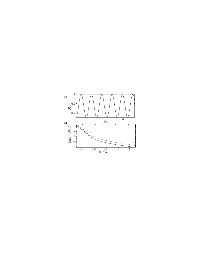
Figure 3: Numerical results in the fast loading limit. (a) The time evolution of the occupation of the lowest ($n=0$) and first excited motional ($n=1$) levels against time in dimensionless units. Note that these lines are indistinguishable. (b) $1-\mathcal{F}_{n}(t=\pi/\Omega)$ after applying a $\pi$-pulse, for the lowest ($n=0$, dotted line) and the first excited ($n=1$, solid line) motional state, as a function of the dimensionless density $n_{\rm 1D}a_{0}$. Parameters used: N=201 particles in the Fermi sea, M=5 lattice sites, $\Omega=17.8\epsilon_{F}$, $\Delta=-3\omega/2$ and in (a) $\omega=0.1~{}\epsilon_{F}$, whereas in (b) $\omega$ is varied.

To model the full loading dynamics we use numerical simulations of the dynamics generated by the Hamiltonian (1). In these simulations we only consider the lowest two motional states for simplicity, but all results are easily extended to more motional states. Also, the simulations are one dimensional, which means that the excited oscillator state with $n=1$ is no longer degenerate. Because couplings to motional excitations in different spatial directions are independent, such simulations are representative for loading into each of the three 3D modes.

In Fig. 3a we show the results of our numerical simulations of the complete system described by the Hamiltonian Eq. (1) in the fast loading limit. In the upper and lower part we plot the fidelity $\mathcal{F}_{m}(t)\equiv\sum_{\alpha}\langle a_{\alpha,m}^{\dagger}a_{\alpha,m}(t)\rangle/M$, with $M$ the number of lattice sites, of the lowest and first excited Bloch band as a function of time in dimensionless units $t\epsilon_{F}$. The numerical results are in excellent agreement with the analytical calculations (Eq. (18)), as we find oscillations of the fidelity in both Bloch bands between zero and $\mathcal{F}_{m}(t)\gtrsim 1-10^{-4}$ occur with a Rabi frequency $\Omega$. In Fig. 3b we analyze the scaling of the fidelity in the two bands with the dimensionless density $n_{3\rm D}a_{0}^{3}$ (i.e., with $n_{1D}a_{0}=\sqrt{2\epsilon_{F}/\omega}/\pi$ in our one dimensional simulations, with $n_{1D}$ the one dimensional density of the reservoir gas). As expected, the fidelity after a $\pi$ pulse, i.e., $\mathcal{F}_{m}(t=\pi/\Omega)$ increases with the density, and high fidelity states can be achieved for large densities $n_{1D}a_{0}\gtrsim 1$. In this and all numerical simulations below we have checked that the results are independent of the quantization volume, which is much smaller than in a real experiment, due to the comparably small number of particles in the simulations.

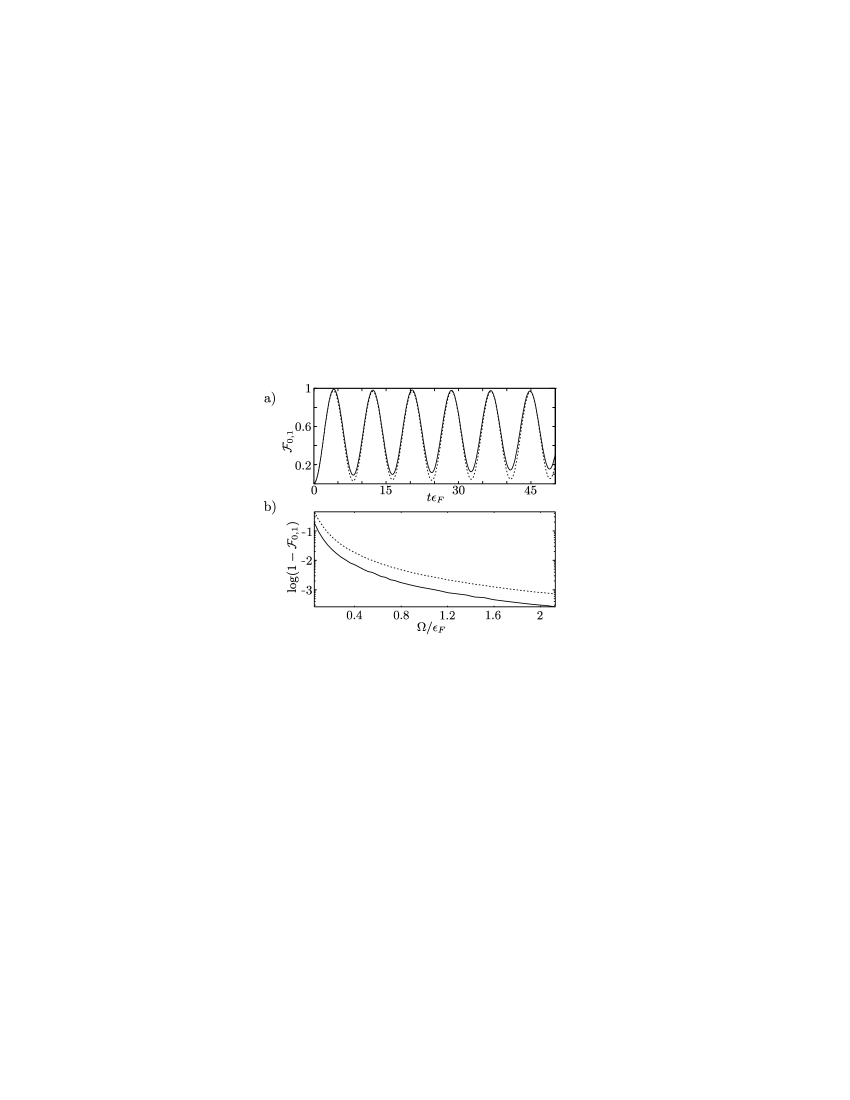
Figure 4: Numerical results for $\Omega$ approaching an intermediate regime from the fast loading limit. (a) The time evolution of the occupation of the lowest ($n=0$, dotted line) and first excited ($n=1$, solid line) motional state against time in dimensionless units, again for $N=101$, $M=5$ and for a typical set of parameters $\Omega=0.72\epsilon_{F}$, $\Delta=-3\omega/2$ and $n_{\rm 1D}a_{0}\sim 2$. (b) The occupation number for the lowest ($n=0$, dotted line) and first excited ($n=1$, solid line) after applying a $\pi$-pulse versus the dimensionless Rabi frequency $\Omega$.

In Fig. 4 we show how the loading dynamics change when approaching the intermediate regime from the fast limit, i.e. the scaling of the fidelity with the Rabi frequency $\Omega$. In Fig. 4a we show the qualitative behaviour of the loading dynamics for typical parameters, in Fig. 4b the scaling of the fidelity $\mathcal{F}_{m}(t=\pi/\Omega)$, $m=0,1$ is shown as a function of the Rabi frequency. These numerical simulations show that the Bloch bands still cannot be individually addressed, and the fidelity becomes worse if the Rabi frequency is decreased.

Thus, our chosen motional state can, in principle, be efficiently filled in this regime on sufficiently fast timescales. However, the requirements on the density are difficult to achieve experimentally, and occupation in other motional states cannot be avoided. As a result in this regime we obtain no significant advantage over traditional loading mechanisms such as adiabatically turning on the lattice. In the next section we will investigate the slow loading regime. In this limit these problems do not exist and we are able to selectively load a single energy level efficiently.

II.3.2 Slow Loading Regime

In this regime, transport is significant during the loading, and the system dynamics are described by the complete Hamiltonian (1). As the reservoir atoms move between Wannier modes during the loading process, it is now more convenient to directly use the momentum representation Eq. (II.1) to express the coupling Hamiltonian.

From Eq. (II.1) one can see that each lattice site $\alpha$ and each motional state ${\mathbf{n}}$ is coupled to many momentum modes $b_{\mathbf{k}}$ in the reservoir. However, as $\Omega\ll\epsilon_{F}$, effectively only a subset of momentum modes with energies centered around the resonant frequency $\epsilon=\Delta+3\omega/2$ is coupled to the lattice, whereas the remaining states are far detuned and the transfer is suppressed. The width of this effective coupling range depends on both the Rabi frequency $\Omega$ and the matrix elements $R_{{\mathbf{k}},{\mathbf{n}}}$, and an upper bound for the width of this range is given by the Rabi frequency $\Omega$.

It is convenient to rewrite the coupling Hamiltonian of Eq. (II.1) as

$$H_{\rm RC}=\sum_{{\mathbf{k}},{\mathbf{n}}}\left[R_{{\mathbf{k}},{\mathbf{n}}}b_{\mathbf{k}}^{\dagger}\left(\sum_{\alpha}{\rm e}^{-{\rm i}{\mathbf{k}}{\mathbf{x}}_{\alpha}}a_{\alpha,{\mathbf{n}}}\right)+{\rm h.c.}\right],$$ (21)

from which we can see that each momentum mode in the reservoir couples to a collective mode $\sum_{\alpha}{\rm e}^{{\rm i}\varphi_{{\mathbf{k}},\alpha}}a_{\alpha,{\mathbf{n}}}$ in the lattice. To fill the lattice it is necessary that the range of states in the reservoir couples to at least $M$ orthogonal collective modes in the lattice. Writing the phase as

$${\mathbf{k}}{\mathbf{x}}_{\alpha}=\pi\sqrt{\frac{\epsilon_{F}}{\omega_{R}}}\left(\frac{{\mathbf{k}}}{k_{F}}\frac{{\mathbf{x}}_{\alpha}}{\lambda/2}\right),$$ (22)

we see that it is necessary to couple a range of states with width of at least $k_{F}\sqrt{\omega_{R}/\epsilon_{F}}$ in momentum space to the lattice to fill $M$ lattice sites. In the slow regime, where $\Omega\ll\epsilon_{F}$ and furthermore $\omega_{R}\lesssim\epsilon_{F}$ (from the density condition (15), the recoil frequency will typically exceed the Rabi frequency, i.e., $\Omega<\omega_{R}$. As only states within a range $\epsilon\pm\Omega$ are coupled to the lattice, the lattice cannot be filled efficiently for a constant $\epsilon$.

Thus to achieve a high population in the desired motional state of each lattice site we must sweep the resonant frequency $\epsilon$ through a range of at least $\omega_{R}$, scanning through many modes. Such a procedure also has the advantage that as we only couple to a narrow range in the Fermi sea at any one time, the reverse process of transferring particles from the lattice to the Fermi sea will be suppressed by Pauli blocking. In our numerical simulations we linearly sweep the detuning from $\epsilon=0$ to $\epsilon=\epsilon_{F}$ in a loading time $T$.

We are interested in the time evolution of the matrix elements $\langle a_{\alpha,n}^{\dagger}a_{\beta,m}\rangle$, $\langle a_{\alpha,n}^{\dagger}b_{\mathbf{k}}\rangle$, and $\langle b_{\mathbf{k}}^{\dagger}b_{{\mathbf{k}}^{\prime}}\rangle$ of the single particle density matrix. For a system described by a quadratic Hamiltonian the equations of motion for the second order correlation functions can be obtained from the (linear) Heisenberg equations (see Appendix A). As the system is described by the quadratic Hamiltonian (1) and (II.1), the linear Heisenberg equations for the operators $a_{\alpha,n}$ and $b_{\mathbf{k}}$ have the simple form (again only considering the lowest two motional states in a one dimensional system)

$$\dot{a}_{\alpha,1}=-{\rm i}\frac{\Omega}{2}\sum_{\mathbf{q}}R_{{\mathbf{q}},1}^{*}{\rm e}^{{\rm i}{\mathbf{k}}{\mathbf{x}}_{\alpha}}b_{\mathbf{q}}-{\rm i}\epsilon a_{\alpha,1},$$

$$\dot{b}_{\mathbf{k}}=-{\rm i}\frac{\Omega}{2}\sum_{\mu,n}R_{{\mathbf{k}},n}{\rm e}^{-{\rm i}{\mathbf{k}}{\mathbf{x}}_{\mu}}a_{\mu,n}-{\rm i}\epsilon_{\mathbf{k}}b_{\mathbf{k}},$$

$$\dot{a}_{\alpha,0}=-{\rm i}\frac{\Omega}{2}\sum_{\mathbf{q}}R_{{\mathbf{q}},0}^{*}{\rm e}^{{\rm i}{\mathbf{k}}{\mathbf{x}}_{\mu}}b_{\mathbf{q}}+{\rm i}(\omega-\epsilon)a_{\alpha,0},$$ (23)

which can be used to efficiently calculate the time evolution of the desired functions numerically. Note that in an isotropic three dimensional lattice again all three degenerate $n=1$ states will be loaded by sweeping the resonant frequency $\epsilon$ through the Fermi sea. In practice it is also possible to selectively load only a single atom in each lattice site by shifting two excited motional states out of resonance, choosing an anisotropic lattice with significantly higher oscillator frequencies in two dimensions.

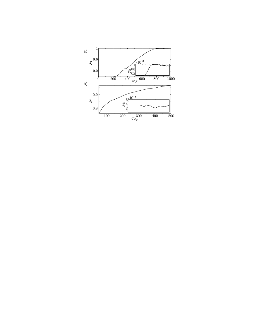
Figure 5: Numerical simulation of the loading dynamics in the “slow loading” limit. (a) Occupation of the lowest and first excited motional bands as a function of time, showing attainment of a high fidelity in the excited band. The resonant frequency $\epsilon$ is swept from $\epsilon_{F}\rightarrow 0$, and $\Omega$ is ramped from $0$ to $0.45\epsilon_{F}$, reaching that value at $t\epsilon_{F}=500$. Parameters used: $N=81$ particles in the Fermi sea, $M=5$ lattice sites, $\omega=5\epsilon_{F}$ and $n_{\rm 1D}\lambda/2=3.4$. (b) The final occupation number after a loading sweep with constant $\Omega$, and $\epsilon$ ramped from $\epsilon_{F}\rightarrow 0$, versus the dimensionless sweep time $\epsilon_{F}T$. Parameters used: $N=81$, $M=5$, $\Omega=0.9\epsilon_{F}$ and $\omega=10\epsilon_{F}$ and $n_{\rm 1D}\lambda/2=1.7$.

In Fig. 5a we show numerical results for the time evolution of the occupation number in the first (upper plot) and in the lowest (lower plot) Bloch band as a function of time in dimensionless units. Here, $\Omega$ is slowly switched on to reduce the additional holes introduced in the Fermi sea by coupling atoms into states above $\epsilon_{F}$. This is an example of many possible optimisations to produce high filling, and we find the final $\mathcal{F}_{1}>0.99$, in a time of the order of $10$ milliseconds (with $\omega\sim 2\pi\times 100$ kHz). In Fig. 5b the occupation of the two motional levels after a loading sweep is plotted as a function of the sweep time $T$. These results are not optimised ($\Omega$ is held constant, and we sweep $\epsilon$ from $\epsilon_{F}\rightarrow 0$), but still produce fidelities $\mathcal{F}_{1}>0.95$ on a timescale of a few milliseconds, and we see that the average filling factor increases with the loading time.

It is important to note that whilst high fidelities can be obtained by optimising the parameters of the sweep, it is not necessary to achieve high filling during this sweep in order to produce high fidelities for the overall loading scheme. In the full scheme with decay of atoms to the ground motional state included, the upper band need never be completely filled at any one time, and removal of atoms via the decay process will lead to further atoms being coupled into the lattice in the upper motional band.

Due to the condition $\Omega\ll\omega$, unwanted coupling to other Bloch bands can be avoided in this regime, by choosing $\epsilon\ll\omega$ (c.f. Fig. 1), as the coupling is then sufficiently far detuned as demonstrated in the lower two plots of Fig. 5. The scaling of the unwanted coupling to the lower band is shown in Fig. 6a, where we plot the occupation of the two Bloch bands after a linear sweep with $\epsilon_{F}T=300$ against the ratio $\omega/\epsilon_{F}$.

In Fig. 6b we show the numerical results when approaching the intermediate regime, i.e, the scaling of the occupation of the two bands after the linear sweep with the Rabi frequency. We find that also here high occupation of the first Bloch band can be achieved, but by increasing the Rabi frequency the unwanted coupling to the lower band also increases, as can be seen in the lower plot of the figure.

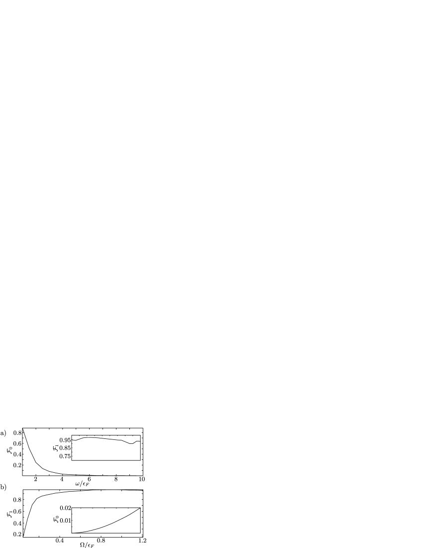
Figure 6: In (a) we show the occupation of the lowest and first excited Bloch band after a linear loading sweep from $\epsilon=\epsilon_{F}\rightarrow 0$ with $\epsilon_{F}T=300$ versus the band separation $\omega$ in dimensionless units. Part (b) shows the loading dynamics approaching an intermediate regime from the slow regime: We plot the occupation of the lowest and first excited Bloch band after a linear loading sweep, with $\epsilon_{F}T=300$ against $\Omega$. Parameters used: N=81 particles in the Fermi Sea, M=5 lattice sites and $n_{\rm 1D}\lambda/2=1.7$, in (a) $\Omega=0.9\epsilon_{F}$ and in (b) $\omega=10\epsilon_{F}$.

In summary, in the “slow loading” regime high fidelity loading of the $n=1$ motional level can be achieved on timescales much shorter than those on which atoms are lost from the lattice by sweeping the resonant coupling frequency $\epsilon$ through the Fermi sea. This loading mechanism gives us the significant advantage over simple loading techniques such as adiabatically increasing the lattice depth that we can address a particular energy level in the lattice, whilst not coupling to levels that are sufficiently far detuned. This property can also be used to load patterns of atoms, because if a superlattice is applied, then the energy of certain lattice sites can be shifted out of resonance with the Raman process, so that no atoms are coupled into these sites.

In the next section we will discuss the cooling of atoms in higher motional levels to the ground state, which removes the atoms from the motional state being coupled from the reservoir. Together with Pauli blocking of modes in the lattice, this allows us to make the overall loading process fault-tolerant. As an additional remark, though, we note that this laser-assisted loading of a selected energy level in the lattice could be used as a stand-alone technique to load the lattice, e.g., coupling atoms directly into the ground motional state. (In order to load an excited motional state in this manner, interaction of atoms in the lattice and atoms in the reservoir must be made very small on the timescale of the loading process, e.g., by using a Feshbach resonance, in order to avoid decay of the atoms into the ground state). This process on its own is not as robust as the procedure we obtain by including a dissipative element in the loading scheme, which will be discussed in the next section. However, reasonably high fidelities could still be obtained with this method alone, especially if the method was applied iteratively, cooling the Fermi reservoir between each two steps. Net transfer of atoms already in the lattice back to the reservoir would be prevented in each step by Pauli blocking in the filled Fermi sea. Note again that as with the full dissipative loading scheme, a single sweep would also not need to completely fill the upper band. The dissipative element discussed in the next section allows for the production of an arbitrarily high-fidelity state without the requirement of iteratively cooling the Fermi reservoir.

III Dissipative Transfer: Cooling Atoms to the Lowest Band

The second stage of the loading process is cooling atoms in an excited motional state to the ground state via interaction with the reservoir gas. This is closely related to the cooling process with a bosonic reservoir in AJ . The external gas here plays the role of an effective $T=0$ heat bath for the lattice atoms, and ground state cooling is achieved on timescales much shorter than atoms are lost from the lattice.

We consider the coupling of lattice atoms $a$ via a collisional interaction to the atoms $b$ in the reservoir so that the system is described by the Hamiltonian

$$H=H_{a}+H_{b}+H_{\rm int},$$ (24)

where the collisional interaction, $H_{\rm int}$, between two fermions is the usual density-density interaction

$$H_{\rm int}=g\int{\rm d}^{3}x\hat{\psi}_{a}^{\dagger}({\mathbf{x}})\hat{\psi}_{a}({\mathbf{x}})\hat{\psi}_{b}^{\dagger}({\mathbf{x}})\hat{\psi}_{b}({\mathbf{x}}),$$ (25)

with $g=4\pi a_{s}/m$ and $a_{s}$ the $s$-wave scattering length. Expanding the field operators as described in the previous section we obtain

$$H_{\rm int}=\sum_{{\mathbf{k}},{\mathbf{k}}^{\prime}\atop\alpha,{\mathbf{n}},{\mathbf{n}}^{\prime}}g_{\alpha,{\mathbf{n}},{\mathbf{n}}^{\prime}}^{{\mathbf{k}},{\mathbf{k}}^{\prime}}b_{{\mathbf{k}}}^{\dagger}b_{{\mathbf{k}}^{\prime}}a_{\alpha,{\mathbf{n}}}^{\dagger}a_{\alpha,{\mathbf{n}}^{\prime}},$$ (26)

which is local in each lattice site because of the small overlap between Wannier functions for neighboring sites in a deep lattice, with

$$g_{\alpha,{\mathbf{n}},{\mathbf{n}}^{\prime}}^{{\mathbf{k}},{\mathbf{k}}^{\prime}}=\frac{g}{V}~{}{\rm e}^{{\rm i}{\mathbf{x}}_{\alpha}({\mathbf{k}}^{\prime}-{\mathbf{k}})}\int{\rm d}^{3}x{\rm e}^{{\rm i}{\mathbf{x}}({\mathbf{k}}^{\prime}-{\mathbf{k}})}w_{\mathbf{n}}({\mathbf{x}})w_{{\mathbf{n}}^{\prime}}({\mathbf{x}}).$$ (27)

Each $g_{\alpha,{\mathbf{n}},{\mathbf{n}}^{\prime}}^{{\mathbf{k}},{\mathbf{k}}^{\prime}}$ describes a scattering process in which a particle-hole pair is created in the reservoir by scattering an atom from momentum state ${\mathbf{k}}\rightarrow{\mathbf{k}}^{\prime}$, combined with the transition of an atom at site $\alpha$ from motional state ${\mathbf{n}}\rightarrow{\mathbf{n}}^{\prime}$.

If the transition in the lattice is from a higher energy mode to a lower energy mode, this corresponds to a cooling transition, whereas the reverse process constitutes heating. As the initial temperature of the reservoir $k_{B}T\ll\epsilon_{F}\ll\omega$, the heating processes will be, at least initially, insignificant, as few reservoir atoms will exist with sufficient energy to excite an atom in the lattice. If the number of atoms in the reservoir is large compared to the number of sites in the lattice ($N\gg M$), then the rate of heating processes due to interaction with previously excited atoms will be small compared to cooling processes due to interaction with atoms remaining below the Fermi energy $\epsilon_{F}$. Because the cooling processes in different lattice sites couple to different modes, and therefore are incoherent, the reservoir can then be treated throughout the process approximately as a $T=0$ bath.

This can be further enhanced in two ways. Firstly, in an experiment in which the reservoir gas is confined in a weak harmonic trap, particles with sufficiently large energies can be allowed to escape from the trap. The large separation of the Bloch band $\omega$, and corresponding excitation energy will then cause many excited reservoir atoms to leave the trap, providing effective evaporative cooling during the process. Secondly, the lattice depth could be modulated during the experiment, so that the excitation energy changes, decreasing the probability that atoms are heated by previously excited reservoir atoms.

The cooling dynamics are then described in the Born-Markov approximation by a Master equation for the reduced density operator $\rho$ for the atoms in the lattice. If we consider coupling of atoms from the first excited motional levels ${\mathbf{n}}\in\{(1,0,0),(0,1,0),(0,0,1)\}$ to the ground state, the resulting master equation (derived in Appendix B) is

$$\dot{\rho}=\sum_{\alpha,\beta,{\mathbf{n}}}\frac{\Gamma_{\alpha,\beta,{\mathbf{n}}}}{2}\left(2A_{\alpha,{\mathbf{n}}}\rho A_{\beta,{\mathbf{n}}}^{\dagger}-A_{\alpha,{\mathbf{n}}}^{\dagger}A_{\beta,{\mathbf{n}}}\rho-\rho A_{\alpha,{\mathbf{n}}}^{\dagger}A_{\beta,{\mathbf{n}}}\right),$$ (28)

with

$$\Gamma_{\alpha,\beta,{\mathbf{n}}}= 2\pi\sum_{{\mathbf{k}},{\mathbf{k}}^{\prime}\atop k^{\prime}>k}g_{\alpha,\bf{1},\bf{0}}^{{\mathbf{k}},{\mathbf{k}}^{\prime}}{g_{\beta,\bf{1},\bf{0}}^{{\mathbf{k}},{\mathbf{k}}^{\prime}}}^{*}\delta\left(\omega-\epsilon_{\mathbf{k}}+\epsilon_{{\mathbf{k}}^{\prime}}\right)$$

$$\approx\frac{g^{2}n_{3\rm D}m}{\pi a_{0}\sqrt{2}}\frac{2}{3e}~{}\delta_{\alpha,\beta}.$$ (29)

Here, the jump operator $A_{\alpha,{\mathbf{n}}}=a_{\alpha,0}^{\dagger}a_{\alpha,{\mathbf{n}}}$ describes the cooling of a lattice atom in site $\alpha$ from the first excited motional level ${\mathbf{n}}$ to the ground state. These results are obtained by calculating the integral over momenta in the Fermi sea to lowest order in $\epsilon_{F}/\omega$.

The approximation in the second line of Eq. (III), in which neglect off diagonal terms $\alpha\not=\beta$ amounts to the approximation that the coherence length of the Fermi reservoir is much shorter than the lattice spacing. This is true provided that the wavelength of the emitted particle excitation, $\sqrt{2\pi^{2}/(m\omega)}$, is much shorter than the lattice spacing, i.e., $\omega_{R}/\omega\ll 1$. This is consistent with the previous approximation that the lattice is so deep that we can neglect tunnelling between neighbouring sites. This can be seen directly when these off-diagonal terms are calculated, as for large $\omega_{R}/\omega$ they decay (to lowest order in $\epsilon_{F}\ll\omega$) as

$$\Gamma_{\alpha,\beta,\mathbf{n}}\sim\frac{\sin(\pi\sqrt{\omega/\omega_{R}}|\alpha-\beta|)}{\pi\sqrt{\omega/\omega_{R}}|\alpha-\beta|}.$$ (30)

This effect is analogous to the spontaneous emission of two excited atoms which are separated spatially by more than one wavelength of the photons they emit. In this case, the atoms can be treated as coupling to two independent reservoirs, and effects of super- and sub-radiance do not play a role.

For typical experimental values $n_{3\rm D}\sim 10^{14}{\rm cm}^{-3}$ and $a_{s}=174a_{B}$, for ⁴⁰K as given in Jin03 , with the Bohr radius $a_{B}$ and a deep optical lattice with $\omega/2\pi\sim 100$kHz, we find a decay rate $\Gamma/2\pi\sim 3.6$kHz. Thus, cooling can again be achieved fast enough, as this rate is much faster than typical loss rates of the lattice atoms. Note, that this value of the decay rate can be made even larger e.g. by tuning the scattering length $a_{s}$ via a Feshbach resonance, as $\Gamma\propto a_{s}^{2}$, by increasing the density of the external gas or by increasing the lattice depth.

In summary we have shown that for a cold reservoir gas with sufficiently many atoms fast ground state cooling of lattice atoms can be achieved with the dissipative coupling of the lattice to the reservoir. The necessary experimental parameters have already been achieved in real experiments, and the cooling rates are tunable via the scattering length and the density of the reservoir gas.

IV Combined Process

The combination of the cooling process with laser-assisted loading in the limit $\Omega\ll\omega,\epsilon_{F}$ will give a final high-fidelity state in the lowest motional level. The primary role of the dissipative element is to transfer atoms into a state in which they are not coupled back to the Fermi reservoir, which is made possible because of the selective addressing of the $n=1$ motional levels in this regime. Multiple occupation of a single site in the lowest motional state is forbidden due to Pauli-blocking, and thus the lowest motional state is monotonically filled; the filling factor and hence the fidelity of the state being prepared always improving in time. Again, patterns of atoms may be loaded in the lowest state by using a superlattice to shift the energy of the $n=1$ motional level out of resonance with the Raman process in particular sites, preventing atoms from being coupled from the Fermi reservoir into those sites. This energy shift will also further suppress tunnelling of atoms from neighbouring sites.

If the laser-assisted loading and the cooling are carried out separately, each being performed after the other in iterative steps, then from the analysis of sections II and III we see that an arbitrarily high fidelity final state can be obtained. This pulsed scheme gives us an upper bound on the timescale for loading a state of given fidelity, which corresponds to the combination of the two individual timescales for laser-assisted loading and cooling. Provided that the number of atoms in the reservoir is much larger than the number of lattice sites to be filled ($N\gg M$), and the Markov approximation made in describing the cooling dynamics is valid, then there will be no adverse effects arising from the loading and cooling processes sharing the same reservoir. Thus, we can combine the two processes into a continuous scheme, which in practice will proceed much faster, as the continuous evacuation of the excited band due to cooling will also speed up the loading process.

At the end of the loading process we must still ensure that the finite occupation of the excited motional levels is properly removed. This can be achieved by detuning the resonant frequency for the Raman coupling above the Fermi energy after the loading sweep, coupling the remaining atoms to empty states above the Fermi sea, and then switching off the coupling adiabatically.

The dynamics of the pulsed process are already well understood from the analysis of sections II and III. To illustrate the dynamics of the combined continuous process, we again perform numerical simulations, in which we compute the matrix elements of the reduced system density operator. The dynamics of the total system including both the laser coupling and the collisional interaction between the optical lattice and the Fermi reservoir are described by the full Hamiltonian

$$H=H_{a}+H_{b}+H_{\rm RC}+H_{\rm int},$$ (31)

and in the Markov approximation with respect to the cooling process, the matrix elements of the system density operator can now be calculated from the Master equation (28) as shown in Appendix C. In order to obtain a closed set of differential equations which can be integrated numerically, we use an approximation based on Wick’s theorem to factorize fourth order correlation functions into second order correlation functions (see appendix C) Simulation .

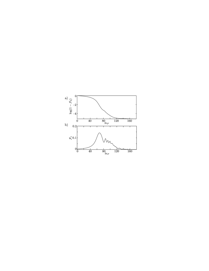
Figure 7: The occupation of (a) the lowest ($n=0$) and (b) first excited ($n=1$) motional level for the continuous combination of coherent loading in the slow regime and dissipative cooling. The resonant frequency is swept from $\epsilon=0$ to $\epsilon=4\epsilon_{F}$ and the Raman coupling is switched off adiabatically. Parameters used: $N=101$, $M=5$, $\Omega/2=0.45\epsilon_{F}$, $n_{\rm 1D}\lambda/2=1.4$, $\omega=10\epsilon_{F}$ and $\Gamma=0.1\epsilon_{F}$.

In Fig. 7 we plot the time evolution of the occupation of the two motional levels in the continuous regime as a function of time. In Fig. 7a we see that we indeed achieve a high occupation of the lowest motional level from the combination of laser-assisted coupling to the excited motional level in the regime $\Omega\ll\omega,\epsilon_{F}$ and cooling to the ground state. For the typical values given in the figure caption, the loading time $T$ for a state with $\mathcal{F}_{0}\sim 1-10^{-4}$ is again on the order of a few milliseconds. This required loading time can be further decreased by tuning $\Gamma$ via the density of the external gas or the strength of the collisional interaction between atoms in the lattice and atoms in the reservoir.

From Fig. 7b we see that as we fill the lower motional level, the filling in the upper level is depleted, and as we continue to tune the lasers so that this level is coupled to states in the reservoir above the Fermi energy $\varepsilon_{F}$, the remaining population in this level is removed.

As a final remark we note that such a procedure could, in principle, also be applied to bosons. However, without Pauli blocking to prevent double-occupation of the ground motional level, we rely on the onsite collisional shift $U$ to make the Raman coupling of an atom from the reservoir into an excited state off-resonant if an atom already exists in the ground motional state. Second order processes occurring at a rate $\sim\Omega\Gamma/U$ can still create double occupation, so we require $\Omega,\Gamma\ll U$, and the advantage of true fault tolerance is not present as it is for fermions.

V Summary

In conclusion, we have shown that the combination of laser-assisted loading of atoms into an excited motional state and the cooling of atoms from this motional state to the ground level gives a fault-tolerant loading scheme to produce high fidelity registers of fermions in an optical lattices with one atom per lattice site. Application of a superlattice allows this to be extended to generalised patterns of atoms, and all of these processes can be completed on timescales much faster than those on which atoms can be lost from the lattice. The advantage of this scheme is that the dissipative transitions in the lattice, similar to optical pumping, gives us a process in which the fidelity of the final state (in the lowest motional level) improves monotonically in time.

Appendix A Derivation of the Heisenberg Equations for Coherent Loading

Consider a system, which is described by a Hamiltonian quadratic in a set of operators $\vec{\mathcal{O}}=(\mathcal{O}_{1},\mathcal{O}_{2},\dots,\mathcal{O}_{d})$. Then the Heisenberg equations of motion can be written as

$$\dot{\vec{\mathcal{O}}}(t)=M\vec{\mathcal{O}}(t),$$ (32)

with a matrix $M$, and formal solution $\vec{\mathcal{O}}(t)=U\vec{\mathcal{O}}(0)$ with $U={\rm exp}(Mt)$. By choosing the initial conditions $\mathcal{O}_{j}(0)=\delta_{j,\alpha}$ we can construct the full time evolution matrix $U(t)$ by solving Eqs. (32), as

$$U_{i,\alpha}(t)\equiv\sum_{j}U_{i,j}(t)\mathcal{O}_{j}(0)=\mathcal{O}_{i}(t).$$ (33)

The time evolution of the second order correlation functions is then easily calculated as

$$\langle\mathcal{O}_{i}^{\dagger}\mathcal{O}_{j}(t)\rangle=\left\langle\sum_{\alpha,\beta}U_{i,j}^{*}(t)U_{j,\beta}(t)\mathcal{O}_{\alpha}^{\dagger}\mathcal{O}_{\beta}(0)\right\rangle.$$ (34)

Appendix B Derivation of the Master Equation

In the interaction picture, and after making the Born-Markov approximation, the master equation for the reduced density operator $\rho$ of a system which interacts with a heat bath via an interaction Hamiltonian $H_{\rm int}$ can be written as (see e.g. QN )

$$\dot{\rho}(t)=-\int_{0}^{t}d\tau\rm{Tr_{B}}\Big{\{}\Big{[}H_{\rm int}(t),\left[H_{\rm int}(t-\tau),\rho(t)\otimes\rho_{B}\right]\Big{]}\Big{\}}.$$ (35)

Here, $\rho_{B}$ is the bath density operator, and $\rm{Tr_{B}}$ denotes the trace over the bath, which is represented by the cold Fermi reservoir in our setup. The interaction between the Fermi reservoir and the optical lattice system is given by the Hamiltonian (26), and in the interaction picture with respect to the internal dynamics in the lattice and in the Fermi reservoir,

$$H_{\rm int}(t)=\sum_{{\mathbf{k}},{\mathbf{k}}^{\prime}\atop\alpha,{\mathbf{n}},{\mathbf{n}}^{\prime}}g_{\alpha,{\mathbf{n}},{\mathbf{n}}^{\prime}}^{{\mathbf{k}},{\mathbf{k}}^{\prime}}b_{{\mathbf{k}}}^{\dagger}b_{{\mathbf{k}}^{\prime}}a_{\alpha,{\mathbf{n}}}^{\dagger}a_{\alpha,{\mathbf{n}}^{\prime}}{\rm e}^{-{\rm i}(\epsilon_{\mathbf{k}}-\epsilon_{{\mathbf{k}}^{\prime}}+\omega(n-n^{\prime}))t}.$$ (36)

As the number of atoms in the reservoir exceeds the number of lattice sites, $N\gg M$, and as in addition the the bath has temperature $T\sim 0$, the reservoir will approximately remain in its ground state, i.e., the filled Fermi sea throughout the cooling process, and the bath correlation functions are approximately given by

$$\langle b_{{\mathbf{k}}_{1}}^{\dagger}b_{{\mathbf{k}}_{1}^{\prime}}b_{{\mathbf{k}}_{2}}^{\dagger}b_{{\mathbf{k}}_{2}^{\prime}}\rangle\approx\delta_{{\mathbf{k}}_{1},{\mathbf{k}}_{1}^{\prime}}\delta_{{\mathbf{k}}_{2},{\mathbf{k}}_{2}^{\prime}}+\delta_{{\mathbf{k}}_{1},{\mathbf{k}}_{2}^{\prime}}\delta_{{\mathbf{k}}_{1}^{\prime},{\mathbf{k}}_{2}},$$ (37)

where $\langle\,\cdot\,\rangle=\rm{Tr_{B}}\{\,\cdot\,\rho_{B}\}$.

For $t$ much larger than the correlation time in the bath we can let the upper limit of the integral in Eq. (35) go to $\infty$, and writing $\int_{0}^{\infty}{\rm e}^{{\rm i}(\epsilon_{\mathbf{k}}-\epsilon_{{\mathbf{k}}^{\prime}}+\omega(n-n^{\prime}))\tau}\rightarrow\delta(\epsilon_{\mathbf{k}}-\epsilon_{{\mathbf{k}}^{\prime}}+\omega(n-n^{\prime}))$, we find

$$\dot{\rho}=\sum_{\alpha,\beta,{\mathbf{n}}}\frac{\Gamma_{\alpha,\beta,{\mathbf{n}}}}{2}\left(2A_{\alpha,{\mathbf{n}}}\rho A_{\beta,{\mathbf{n}}}^{\dagger}-A_{\alpha,{\mathbf{n}}}^{\dagger}A_{\beta,{\mathbf{n}}}\rho-\rho A_{\alpha,{\mathbf{n}}}^{\dagger}A_{\beta,{\mathbf{n}}}\right),$$ (38)

with the jump operator $A_{\alpha,{\mathbf{n}}}=a_{\alpha,0}^{\dagger}a_{\alpha,{\mathbf{n}}}$,

$$\Gamma_{\alpha,\beta,{\mathbf{n}}}= 2\pi\sum_{{\mathbf{k}},{\mathbf{k}}^{\prime}\atop k^{\prime}>k}g_{\alpha,\bf{1},\bf{0}}^{{\mathbf{k}},{\mathbf{k}}^{\prime}}{g_{\beta,\bf{1},\bf{0}}^{{\mathbf{k}},{\mathbf{k}}^{\prime}}}^{*}\delta\left(\omega-\epsilon_{\mathbf{k}}+\epsilon_{{\mathbf{k}}^{\prime}}\right),$$ (39)

and where we note that $\sum_{{\mathbf{k}},{\mathbf{k}}^{\prime}}g_{\alpha,{\mathbf{n}},\bf{0}}^{{\mathbf{k}},{\mathbf{k}}^{\prime}}g_{\alpha,{\mathbf{n}}^{\prime},\bf{0}}^{{\mathbf{k}},{\mathbf{k}}^{\prime}}=0$ for ${\mathbf{n}}\not={\mathbf{n}}^{\prime}$. The rate $\Gamma_{\alpha,\beta,{\mathbf{n}}}$ rapidly decays with $|\alpha-\beta|$, and for each of the three degenerate excited states ${\mathbf{n}}\in\{(1,0,0),(0,1,0),(0,0,1)\}$, the slowest rate of this decay is found in the direction of ${\mathbf{n}}$. In the harmonic oscillator approximation we find (for the direction with the slowest decay)

$$\Gamma_{\alpha,\beta}\sim\frac{g^{2}n_{3\rm D}m}{\pi a_{0}\sqrt{2}}\frac{2}{3e}F(\pi\sqrt{\frac{\omega}{\omega_{R}}}|\alpha-\beta|),$$ (40)

to first order in $\epsilon_{F}/\omega$, with the function

$$F(\xi)=3\frac{2\xi\cos\xi+(\xi^{2}-2)\sin\xi}{\xi^{3}}.$$ (41)

For large $\xi$ this result simplifies to the sinc function in Eq. (30). For a deep optical lattice where $\omega\gg\omega_{R}$, $F(\pi\sqrt{\frac{\omega}{\omega_{R}}}|\alpha-\beta|)\approx\delta_{\alpha,\beta}$, and we end up with a standard quantum optical master equation (see e.g. QN ), describing the decay of an excited lattice atom from each of the three degenerate $n=1$ states to the $n=0$ level at a rate $\Gamma$.

Appendix C Equations of motion for Combined Dynamics

The time evolution of the expectation value of an arbitrary system operator $\hat{\mathcal{O}}$ can be calculated from the master equation (28) and Eq. (III) as

$$\langle\dot{\hat{\mathcal{O}}}\rangle= {\rm i}\langle[H_{\rm sys},\hat{\mathcal{O}}]\rangle+$$

$$+\frac{\Gamma}{2}\sum_{\alpha,{\mathbf{n}}}\left(2\langle A_{\alpha,{\mathbf{n}}}^{\dagger}\hat{\mathcal{O}}A_{\alpha,{\mathbf{n}}}\rangle-\langle\{\hat{\mathcal{O}},A_{\alpha,{\mathbf{n}}}^{\dagger}A_{\alpha,{\mathbf{n}}}\}\rangle\right),$$ (42)

where $H_{\rm sys}=H_{a}+H_{b}+H_{\rm RC}$ and $\Gamma\equiv\Gamma_{\alpha,\alpha,\bf{1}}$. We are interested in the time evolution of the matrix elements of the single particle density matrix, which can be calculated from Eq. (C) as

$$\frac{\rm d}{\rm dt}\langle a_{\alpha,0}^{\dagger}a_{\beta,0}\rangle= {\rm i}\frac{\Omega}{2}\sum_{\mathbf{q}}\left(R_{{\mathbf{q}},\alpha,0}\langle b_{\mathbf{q}}^{\dagger}a_{\beta,0}\rangle-R_{{\mathbf{q}},\beta,0}^{*}\langle a_{\alpha,0}^{\dagger}b_{\mathbf{q}}\rangle\right)+\frac{\Gamma}{2}\left(2\langle a_{\alpha,1}^{\dagger}a_{\alpha,1}\rangle\delta_{\alpha,\beta}-\langle a_{\alpha,1}^{\dagger}a_{\alpha,0}^{\dagger}a_{\beta,0}a_{\alpha,1}\rangle-\langle a_{\beta,1}^{\dagger}a_{\alpha,0}^{\dagger}a_{\beta,0}a_{\beta,1}\rangle\right)$$ (43)

$$\frac{\rm d}{\rm dt}\langle a_{\alpha,1}^{\dagger}a_{\beta,1}\rangle= {\rm i}\frac{\Omega}{2}\sum_{\mathbf{q}}\left(R_{{\mathbf{q}},\alpha,1}\langle b_{\mathbf{q}}^{\dagger}a_{\beta,1}\rangle-R_{{\mathbf{q}},\beta,1}^{*}\langle a_{\alpha,1}^{\dagger}b_{\mathbf{q}}\rangle\right)-\frac{\Gamma}{2}\left(2\langle a_{\alpha,1}^{\dagger}a_{\beta,1}\rangle-\langle a_{\alpha,1}^{\dagger}a_{\beta,0}^{\dagger}a_{\beta,0}a_{\beta,1}\rangle-\langle a_{\alpha,1}^{\dagger}a_{\alpha,0}^{\dagger}a_{\alpha,0}a_{\beta,1}\rangle\right)$$

$$\frac{\rm d}{\rm dt}\langle a_{\alpha,1}^{\dagger}a_{\beta,0}\rangle= {\rm i}(\omega-\epsilon)\langle a_{\alpha,1}^{\dagger}a_{\beta,0}\rangle+{\rm i}\frac{\Omega}{2}\sum_{\mathbf{q}}\left(R_{{\mathbf{q}},\alpha,1}\langle b_{\mathbf{q}}^{\dagger}a_{\beta,0}\rangle-R_{{\mathbf{q}},\beta,0}^{*}\langle a_{\alpha,1}^{\dagger}b_{\mathbf{q}}\rangle\right)$$

$$+\frac{\Gamma}{2}\left(-\langle a_{\alpha,1}^{\dagger}a_{\beta,0}\rangle-\langle a_{\alpha,1}^{\dagger}a_{\beta,1}^{\dagger}a_{\beta,1}a_{\beta,0}\rangle-\langle a_{\alpha,1}^{\dagger}a_{\alpha,0}^{\dagger}a_{\alpha,0}a_{\beta,0}\rangle\right)$$

$$\frac{\rm d}{\rm dt}\langle a_{\alpha,1}^{\dagger}b_{\mathbf{k}}\rangle= {\rm i}(\epsilon-\epsilon_{\mathbf{k}})\langle a_{\alpha,1}^{\dagger}b_{\mathbf{k}}\rangle+{\rm i}\frac{\Omega}{2}\left(\sum_{\mathbf{q}}R_{{\mathbf{q}},\alpha,1}\langle b_{\mathbf{q}}^{\dagger}b_{\mathbf{k}}\rangle-\sum_{\mu}R_{{\mathbf{k}},\mu,1}\langle a_{\alpha,1}^{\dagger}a_{\mu,1}\rangle\right)-\frac{\Gamma}{2}\left(\langle a_{\alpha,1}^{\dagger}b_{\mathbf{k}}\rangle+\langle a_{\alpha,1}^{\dagger}a_{\alpha,0}^{\dagger}a_{\alpha,0}b_{\mathbf{k}}\rangle\right)$$

$$\frac{\rm d}{\rm dt}\langle a_{\alpha,0}^{\dagger}b_{\mathbf{k}}\rangle= {\rm i}(\epsilon-\epsilon_{\mathbf{k}}-\omega)\langle a_{\alpha,0}^{\dagger}b_{\mathbf{k}}\rangle+{\rm i}\frac{\Omega}{2}\left(\sum_{\mathbf{q}}R_{{\mathbf{q}},\alpha,0}\langle b_{\mathbf{q}}^{\dagger}b_{\mathbf{k}}\rangle-\sum_{\mu}R_{{\mathbf{k}},\mu,0}\langle a_{\alpha,0}^{\dagger}a_{\mu,0}\rangle\right)-\frac{\Gamma}{2}\langle a_{\alpha,1}^{\dagger}a_{\alpha,0}^{\dagger}b_{\mathbf{k}}a_{\alpha,1}\rangle$$

$$\frac{\rm d}{\rm dt}\langle b_{\mathbf{k}}^{\dagger}b_{{\mathbf{k}}^{\prime}}\rangle= {\rm i}(\epsilon_{\mathbf{k}}-\epsilon_{{\mathbf{k}}^{\prime}}-\omega)\langle b_{\mathbf{k}}^{\dagger}b_{{\mathbf{k}}^{\prime}}\rangle+{\rm i}\frac{\Omega}{2}\sum_{\mu,n}\left(-R_{{\mathbf{k}},\mu,n}\langle b_{\mathbf{k}}^{\dagger}a_{\mu,n}\rangle-R_{{\mathbf{k}},\mu,n}^{*}\langle a_{\mu,n}^{\dagger}b_{{\mathbf{k}}^{\prime}}\rangle\right).$$

A closed set of equations can be obtained from Eqs. (43) by using Wick’s theorem to factorize fourth order correlation functions into products of second order correlation functions according to

$$\langle\hat{c_{1}}\hat{c_{2}}\hat{c_{4}}\hat{c_{4}}\rangle=\langle\hat{c_{1}}\hat{c_{2}}\rangle\langle\hat{c_{3}}\hat{c_{4}}\rangle-\langle\hat{c_{1}}\hat{c_{3}}\rangle\langle\hat{c_{2}}\hat{c_{4}}\rangle+\langle\hat{c_{1}}\hat{c_{4}}\rangle\langle\hat{c_{2}}\hat{c_{3}}\rangle,$$

for fermionic operators $\hat{c_{i}}\in\{a_{\alpha,{\mathbf{n}}}^{\dagger},a_{\alpha,{\mathbf{n}}},b_{\mathbf{k}}^{\dagger},b_{\mathbf{k}}\}$ (see e.g. Castin_BEC ).

References

- (1) For a review see D. Jaksch and P. Zoller, Annals of Physics 315, 52 (2005), and references therein.
- (2) M. Greiner, O. Mandel, T. W. Hänsch and I. Bloch Nature 415, 39 (2002); M. Greiner, O. Mandel, T. Esslinger, T.W. Hänsch and I. Bloch, Nature 419 51 (2002).
- (3) T. Stöferle, H. Moritz, C. Schori, M. Köhl, and T. Esslinger, Phys. Rev. Lett. 92 130403 (2004).
- (4) B. Paredes, A. Widera, V. Murg, O. Mandel, S. Fölling, I. Cirac, G. V. Shlyapnikov, T. W. Hänsch, and I. Bloch, Nature 429, 277 (2004).
- (5) O. Mandel, M. Greiner, A. Widera, T. Rom, T. W. Hänsch, and I. Bloch, Phys. Rev. Lett. 91, 010407 (2003).
- (6) E. L. Bolda, E. Tiesinga, and P. S. Julienne, Phys. Rev. A 66, 013403; E. A. Donley, N. R. Claussen, S. T. Thompson, and C. E. Wieman, Nature 417, 529 (2002); T. Loftus, C. A. Regal, C. Ticknor, J. L. Bohn, and D. S. Jin, Phys. Rev. Lett. 88, 173201 (2002).
- (7) M. Theis, G. Thalhammer, K. Winkler, M. Hellwig, G. Ruff, R. Grimm, J. Hecker Denschlag, Phys. Rev. Lett. 93, 123001 (2004).
- (8) P. Rabl, A. J. Daley, P. O. Fedichev, J. I. Cirac, and P. Zoller, Phys. Rev. Lett. 91, 110403 (2003).
- (9) I.H. Deutsch, G.K. Brennen, and P.S. Jessen, Fortschritte der Physik 48, 925 (2000).
- (10) For example see L. Santos, M. A. Baranov, J. I. Cirac, H.-U. Everts, H. Fehrmann, and M. Lewenstein, Phys. Rev. Lett. 93 030601 (2004).
- (11) D. Jaksch, C. Bruder, J. I. Cirac, C. W. Gardiner, and P. Zoller, Phys. Rev. Lett. 81, 3108 (1998).
- (12) L. Viverit, C. Menotti, T. Calarco, A. Smerzi, Phys. Rev. Lett. 93, 110401 (2004).
- (13) K. G. H. Vollbrecht, E. Solano, and J. I. Cirac, Phys. Rev. Lett. 93, 220502 (2004).
- (14) G. K. Brennen, G. Pupillo, A. M. Rey, C. W. Clark, and C. J. Williams, quant-ph/0312069.
- (15) D. S. Weiss, J. Vala, A. V. Thapliyal, S. Myrgren, U. Vazirani, and K. B. Whaley, Phys. Rev. A 70, 040302(R) (2004).
- (16) B. DeMarco and D. S. Jin, Science 285, 1703 (1999).
- (17) S. Jochim, M. Bartenstein, A. Altmeyer, G. Hendl, S. Riedl, C. Chin, J. Hecker Denschlag, and R. Grimm, Science 302, 2101 (2003).
- (18) M. Greiner, C. A. Regal, and D. S. Jin, Nature 426, 537 (2003).
- (19) M. W. Zwierlein, C. A. Stan, C. H. Schunck, S. M. F. Raupach, A. J. Kerman, and W. Ketterle, Phys. Rev. Lett. 92, 120403 (2004).
- (20) G. Roati, F. Riboli, G. Modugno, and M. Inguscio, Phys. Rev. Lett. 89, 150403 (2002).
- (21) M. Köhl, H. Moritz, T. Stöferle, K. Günter, and T. Esslinger, cond-mat/0410389.
- (22) T. Bourdel, L. Khaykovich, J. Cubizolles, J. Zhang, F. Chevy, M. Teichmann, L. Tarruell, S. J. J. M. F. Kokkelmans, and C. Salomon, Phys. Rev. Lett. 93, 050401 (2004).
- (23) K. E. Strecker, G. B. Partridge, and R. G. Hulet, Phys. Rev. Lett. 91, 080406 (2003).
- (24) J. Kinast, S. L. Hemmer, M. E. Gehm, A. Turlapov, and J. E. Thomas, Phys. Rev. Lett. 92, 150402 (2004).
- (25) W. Hofstetter, J. I. Cirac, P. Zoller, E. Demler, and M. D. Lukin, Phys. Rev. Lett. 89, 220407 (2002).
- (26) B. Mohring, M. Bienert, F. Haug, G. Morigi, W. P. Schleich, and M. G. Raizen, quant-ph/0412181; R. B. Diener, B. Wu, M. G. Raizen, and Q. Niu, Phys. Rev. Lett 89, 070401 (2002).
- (27) A. J. Daley, P. O. Fedichev, and P. Zoller Phys. Rev. A 69, 022306 (2004).
- (28) C. A. Regal and D. S. Jin, Phys. Rev. Lett. 90, 230404 (2003).
- (29) This problem could, in principle, be treated exactly using new methods for simulation of dissipative D systems, as discussed in M. Zwolak and G. Vidal, Phys. Rev. Lett. 93, 207205 (2004); F. Verstraete, J. J. Garcia-Ripoll, and J. I. Cirac, Phys. Rev. Lett. 93, 207204 (2004).
- (30) C. W. Gardiner and P. Zoller, Quantum Noise, Springer (2000).
- (31) Y. Castin, cond-mat/0407118 (2004).