New method to simulate quantum interference using deterministic processes and application to event-based simulation of quantum computation

Abstract

We demonstrate that networks of locally connected processing units with a primitive learning capability exhibit behavior that is usually only attributed to quantum systems. We describe networks that simulate single-photon beam-splitter and Mach-Zehnder interferometer experiments on a causal, event-by-event basis and demonstrate that the simulation results are in excellent agreement with quantum theory. We also show that this approach can be generalized to simulate universal quantum computers.

1 Introduction

Computer simulation is a powerful methodology to model physical phenomena [1]. However, some of the most fundamental experiments in quantum physics [2, 3] have not been simulated in the event-by-event manner in which the experimental observations are actually recorded [4]. In experiments the detection of events appears to be random [2, 3], in a sense which, as far as we know, has not been studied systematically. Quantum theory gives us a recipe to compute the frequency of the observation of events but it does not describe individual events, such as the arrival of a single electron at a particular position on the detection screen [3, 5, 6, 7]. Reconciling the mathematical formalism (that does not describe single events) with the experimental fact that each observation yields a definite outcome is often referred to as the quantum measurement paradox. This is a central, fundamental problem in the foundation of quantum theory [6, 5, 8]. Therefore, it is not a such a surprise that within the framework of quantum theory, no algorithm has been found to perform an event-based simulation of quantum phenomena.

From a computational viewpoint, quantum theory provides us with a set of rules (algorithms) to compute probability distributions [5, 9, 10]. Therefore we may wonder what kind of algorithm(s) we need to perform an event-based simulation of the experiments [2, 3] mentioned above without using the machinery of quantum theory. Evidently, the present formulation rules out any method based on the solution of the (time-dependent) Schrödinger equation and we have to step outside the framework that quantum theory provides.

In this paper we demonstrate that locally-connected networks of processing units with a primitive learning capability are sufficient to simulate deterministically and event-by-event, the single-photon beam splitter and Mach-Zehnder interferometer experiments of Grangier et al. [2]. We also show that this approach can be generalized to simulate universal quantum computation by a deterministic event-by-event process. Thus, the method we propose can simulate wave interference phenomena and many-body quantum systems using classical, particle-like processes only.

Our results suggest that we may have discovered a procedure to simulate quantum phenomena using causal, local, deterministic and event-based processes. Our approach is not an extension of quantum theory in any sense and is not a proposal for another interpretation of quantum mechanics. The probability distributions of quantum theory are generated by a deterministic, causal learning process, and not vice versa [8].

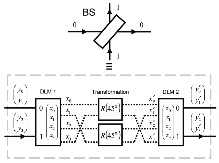
Figure 1: Diagram of the network of two DLMs that performs a deterministic simulation of a single-photon beam splitter (BS) on an event-by-event basis [11]. The solid lines represent the input and output channels of the BS. Dashed lines indicate the flow of data within the BS. Input channel 0 receives $(y_{0},y_{1})=(\cos\psi_{0},\sin\psi_{0})$ with probability $p_{0}$. Input channel 1 receives $(y_{2},y_{3})=(\cos\psi_{1},\sin\psi_{1})$ with probability $p_{1}=1-p_{0}$. $R(45^{\circ})$ denotes a rotation of a two-dimensional vector by $45^{\circ}$ (see Eq. (5)).

2 Deterministic Learning Machine (DLM) [11]

In quantum physics, an event corresponds to the detection of a photon, electron, and the like. In our simulation approach an event is the arrival of a message at the input channel of a processing unit. This processing unit typically contains two DLMs (described below). We use the diagram of a DLM-based processor that performs the event-by-event simulation of single-photon beam splitter, as shown in Fig. 1, to describe the operation of the different components of the processor. The applications to quantum computations presented later demonstrate that the structure of the DLM-based processor is in fact generic.

In Fig. 1, the presence of a message is indicated by an arrow on the corresponding line. The first component, DLM 1, “learns” about the occurrence of an event on one of its two input channels that we label with 0 and 1. For brevity, we refer to an event on channel 0 (1) as a 0 (1) event. The second component transforms the data stored in DLM 1 and feeds the result into DLM 2. DLM 2 “learns” this data. Finally the learning process itself is used to determine whether DLM 2 responds to the input event by sending out either a 0 or a 1 event. None of these components makes use of random numbers, hence the name deterministic learning machine.

Usually, DLM-based simulation algorithms contain several DLM-based processors that form a network. In this paper we only consider networks of processing units in which only one message is traveling through the network at any time. Thus, the network receives an event at one of its inputs, processes the event and delivers the processed message through one of its output channels. After delivering this message the network can accept a new input event.

2.1 Description of a DLM

A DLM is a very simple, classical dynamical system with a primitive learning capability. This dynamical system consists of a unit vector (such as ${\bf x}=(x_{0},x_{1},x_{2},x_{3})$ in DLM 1 of Fig. 1), a rule that specifies how this vector changes when an input event is received, and a rule by which the DLM determines the type of output event it generates as a response to the input event. The initial value of the internal vectors is irrelevant. In simulations, we usually use random numbers to initialize the internal vectors of all the DLMs in the network.

We now describe the learning process of a DLM in detail [12]. The basic idea of the learning algorithm is that the DLM minimizes the distance between the input vector (discussed later) and the internal vector and that this minimization is sufficient to construct particle-like processes that mimic quantum phenomena. However, the algorithm that we describe below cannot be derived from the axioms of quantum theory. After many trials and failures, we simply discovered that learning algorithms of this type can be used to simulate quantum phenomena.

First we consider DLM 1 in Fig. 1. The internal state of DLM 1 is represented by the vector ${\bf x}=(x_{0},x_{1},x_{2},x_{3})$. DLM 1 can accept two different types of input events, but only one at a time. Event 0 carries a message represented by a two-dimensional unit vector $(y_{0},y_{1})$. Event 1 carries a message represented by a two-dimensional unit vector $(y_{2},y_{3})$. Upon receiving an input event, DLM 1 performs the following steps:

• DLM 1 computes eight candidate internal states

  $${\bf w}_{1} = (+\sqrt{1-\alpha^{2}+\alpha^{2}x_{0}^{2}},\alpha x_{1},\alpha x_{2},\alpha x_{3}),$$

  $${\bf w}_{2} = (-\sqrt{1-\alpha^{2}+\alpha^{2}x_{0}^{2}},\alpha x_{1},\alpha x_{2},\alpha x_{3}),$$

  $${\bf w}_{3} = (\alpha x_{0},+\sqrt{1-\alpha^{2}+\alpha^{2}x_{1}^{2}},\alpha x_{2},\alpha x_{3}),$$

  $${\bf w}_{4} = (\alpha x_{0},-\sqrt{1-\alpha^{2}+\alpha^{2}x_{1}^{2}},\alpha x_{2},\alpha x_{3}),$$

  $${\bf w}_{5} = (\alpha x_{0},\alpha x_{1},+\sqrt{1-\alpha^{2}+\alpha^{2}x_{2}^{2}},\alpha x_{3}),$$

  $${\bf w}_{6} = (\alpha x_{0},\alpha x_{1},-\sqrt{1-\alpha^{2}+\alpha^{2}x_{2}^{2}},\alpha x_{3}),$$

  $${\bf w}_{7} = (\alpha x_{0},\alpha x_{1},\alpha x_{2},+\sqrt{1-\alpha^{2}+\alpha^{2}x_{3}^{2}}),$$

  $${\bf w}_{8} = (\alpha x_{0},\alpha x_{1},\alpha x_{2},-\sqrt{1-\alpha^{2}+\alpha^{2}x_{3}^{2}}).$$ (1)

  The parameter $0<\alpha<1$ controls the learning process and is discussed in more detail later. The plus and minus sign in front of the square roots is introduced to allow the vector ${\bf w}_{j}$ to cover the whole eight-dimensional unit sphere.

• If DLM 1 receives an input event of type 0 with message $(y_{0},y_{1})$, it constructs a vector ${\bf\hat{x}}=(y_{0},y_{1},x_{2},x_{3})$. If DLM 1 receives an input event of type 1 with message $(y_{2},y_{3})$, it constructs a vector ${\bf\hat{x}}=(x_{0},x_{1},y_{2},y_{3})$. DLM 1 determines the update rule $m$ that minimizes the cost function

  $$C_{j}=-{\bf w}_{j}^{T}{\bf\hat{x}},$$ (2)

  that is, $C_{m}\leq C_{j}$ for $j=1,\ldots,8$.

• DLM 1 updates its internal vector by replacing ${\bf x}$ by ${\bf w}_{m}$.

• DLM 1 generates a new (internal) event by putting the values of its internal vector on its four output channels.

• DLM 1 waits for the arrival of the next input event.

The transformation stage applies an orthogonal transformation $T$ to ${\bf x}=(x_{0},x_{1},x_{2},x_{3})$. In general, the precise form of the transformation $T$ depends on the particular function that the processor has to perform. In the example shown in Fig. 1, the orthogonal transformation $T$ takes two pairs of elements from ${\bf x}$ and performs the plane rotation

$$R(\phi)=\left(\begin{array}[]{cc}\cos\phi&-\sin\phi\\ \sin\phi&\phantom{-}\cos\phi\end{array}\right),$$ (5)

with $\phi=\pi/4$. As we show later, this transformation implements the single-photon beam splitter. The result ${\bf x^{\prime}}=(x_{0}^{\prime},x_{1}^{\prime},x_{2}^{\prime},x_{3}^{\prime})$ of this transformation is sent to the input of DLM 2. Thus, DLM 2 accepts messages in the form of a four-dimensional unit vector. DLM 2 updates its internal vector ${\bf z}=(z_{0},z_{1},z_{2},z_{3})$ according to the following procedure:

• DLM 2 performs computes eight candidate internal states

  $${\bf w}_{1} = (+\sqrt{1-\alpha^{2}+\alpha^{2}z_{0}^{2}},\alpha z_{1},\alpha z_{2},\alpha z_{3}),$$

  $${\bf w}_{2} = (-\sqrt{1-\alpha^{2}+\alpha^{2}z_{0}^{2}},\alpha z_{1},\alpha z_{2},\alpha z_{3}),$$

  $${\bf w}_{3} = (\alpha z_{0},+\sqrt{1-\alpha^{2}+\alpha^{2}z_{1}^{2}},\alpha z_{2},\alpha z_{3}),$$

  $${\bf w}_{4} = (\alpha z_{0},-\sqrt{1-\alpha^{2}+\alpha^{2}z_{1}^{2}},\alpha z_{2},\alpha z_{3}),$$

  $${\bf w}_{5} = (\alpha z_{0},\alpha z_{1},+\sqrt{1-\alpha^{2}+\alpha^{2}z_{2}^{2}},\alpha z_{3}),$$

  $${\bf w}_{6} = (\alpha z_{0},\alpha z_{1},-\sqrt{1-\alpha^{2}+\alpha^{2}z_{2}^{2}},\alpha z_{3}),$$

  $${\bf w}_{7} = (\alpha z_{0},\alpha z_{1},\alpha z_{2},+\sqrt{1-\alpha^{2}+\alpha^{2}z_{3}^{2}}),$$

  $${\bf w}_{8} = (\alpha z_{0},\alpha z_{1},\alpha z_{2},-\sqrt{1-\alpha^{2}+\alpha^{2}z_{3}^{2}}).$$ (6)

• DLM 2 determines the update rule $m$ that minimizes the cost function

  $$C_{j}=-{\bf w}_{j}^{T}{\bf x}^{\prime},$$ (7)

  that is, $C_{m}\leq C_{j}$ for $j=1,\ldots,8$.

• DLM 2 updates its internal vector by replacing ${\bf z}$ by ${\bf w}_{m}$.

• DLM 2 generates an output event of type 0 (1) if $m=1,\ldots,4$ $(5,\ldots,8)$, carrying the message $(y_{0}^{\prime},y_{1}^{\prime})=(z_{0},z_{1})$ ($(y_{0}^{\prime},y_{1}^{\prime})=(z_{2},z_{3})$).

• DLM 2 waits for the arrival of the next input event.

Comparing the algorithms for DLM 1 and DLM 2, we see that they are indentical except for part of the second step and the fourth step in which the output is generated.

2.2 Dynamic behavior of a DLM

In general, the behavior of a DLM defined by rules Eqs. (1) and (2) or Eqs. (6) and (7) is difficult to analyze without the use of a computer. However, for a fixed input ${\bf x}^{\prime}={\bf u}$, it is clear what a DLM will do. It will minimize the cost given by Eq. (7) by rotating its internal vector ${\bf z}$ to bring it as close as possible to ${\bf u}$. After a number of events (depending on the initial value of ${\bf z}$, the input ${\bf u}$, and $\alpha$), ${\bf z}$ will be close to ${\bf u}$. However, the vector ${\bf z}$ does not converge to a limiting value because the DLM always changes its internal vector state by a nonzero amount. It is not difficult to see (and supported by simulations, results not shown) that once ${\bf z}$ is close to ${\bf u}$, it will keep oscillating about ${\bf u}$ [12]. Below we analyse this behavior in more detail using DLM 2 as an example. The dynamics of DLM 1 is the same as that of DLM 2.

Let us denote by $n_{0}$ the number of times the DLM selects update rule $m=1,2$ (see Eq.(6)). Writing

$$w^{2}_{0,m}=1-\alpha^{2}+\alpha^{2}z_{0}^{2}\equiv(z_{0}+\delta)^{2},$$ (8)

and assuming that $0\ll\alpha<1$, we find that the variable $z_{0}$ changes by an amount

$$\delta\approx(1-\alpha^{2})(1-z_{0}^{2})/2z_{0},$$ (9)

where we have neglected terms of order $\delta^{2}$. Similarily, if $N$ is the total number of events then $N-n_{0}$ is the number of times the DLM selects update rules $m\not=1,2$. For $j\not=1,2$, Eq.(6) gives

$$w^{2}_{0,j}=\alpha^{2}z_{0}^{2}\equiv(z_{0}+\delta^{\prime})^{2},$$ (10)

where we have neglected terms of order ${\delta^{\prime}}^{2}$. Hence $z_{0}$ changes by

$$\delta^{\prime}\approx-(1-\alpha^{2})z_{0}/2.$$ (11)

If ${\bf z}$ oscillates about ${\bf u}$ then $z_{0}$ also oscillates about ${u}_{0}$. This implies that the number of times $z_{0}$ increases times the increment must approximately be equal to the number of times $z_{0}$ decreases times the decrement. In other words, we must have $n_{0}\delta+(N-n_{0})\delta^{\prime}\approx 0$. As $z_{0}\approx{u}_{0}$ we conclude that $n_{0}/N\approx{u}_{0}^{2}$. Applying the same reasoning for the cases where the DLM selects update rule $m=3,4$ shows that the number of times the DLM will apply update rules $m=3,4$ is proportional to ${u}_{0}^{2}+{u}_{1}^{2}$.

At this point, there is not yet a relation between the dynamics of the DLM and quantum theory. However, let us now assume that $p_{0}=z_{0}^{2}+z_{1}^{2}$ ($p_{1}=z_{2}^{2}+z_{3}^{2}$) is the probability that a quantum system is observed to be in the state 0 (1). In quantum theory, we would describe this state by a wave function with complex amplitudes $\hat{z}_{0}+i\hat{z}_{1}$ ($\hat{z}_{2}+i\hat{z}_{3}$). Let is now consider a DLM that is learning the four values ${\bf z}=(z_{0},z_{1},z_{2},z_{3})$. From the foregoing discussion, it follows that once the DLM has reached the stationary state in which it oscillates about ${\bf z}$, the rate at which the DLM uses update rules $m=1,2,3,4$ ($m=5,6,7,8$) corresponds to the probability $p_{0}$ ($p_{1}$) to observe a 0 (1) event in the quantum mechanical system. Thus, the DLM generates 0 and 1 events in a deterministic manner and because it generates 0 (1) events if it selected update rule $m=1,2,3,4$ $(5,6,7,8)$, the rate at which these events are generated agrees with the corresponding probabilities of quantum theory. As the applications presented later demonstrate, this correspondence is all that is needed to perform an event-by-event simulation of quantum interference and many-body quantum phenomena.

Figure 2: Simulation results for the beam splitter shown in Fig. 1. Markers give the simulation results for the normalized intensity $N_{0}/(N_{0}+N_{1})$ in output channel 0 as a function of $\phi=\psi_{0}-\psi_{1}$. Open circles: $p_{0}=1$; Bullets: $p_{0}=0.5$; Open squares: $p_{0}=0.25$. The results of quantum theory $|b_{0}|^{2}$ (see Eq. (19)) are represented by lines.

2.3 Stochastic variant

The sequence of events that is generated by a DLM (network) is strictly deterministic but a simple modification turns a DLM into a stochastic learning machine (SLM). The term stochastic does not refer to the learning process but to the method that is used to select the output channel that will carry the outgoing message. As explained earlier, in the stationary regime $x_{0}^{2}+x_{1}^{2}$ and $x_{2}^{2}+x_{3}^{2}$ (or $z_{0}^{2}+z_{1}^{2}$ and $z_{2}^{2}+z_{3}^{2}$) correspond to the probabilities of quantum theory. Thus, a comparision of for instance, $x_{0}^{2}+x_{1}^{2}$, with a uniform random number $0<r<1$ gives the probability for sending the message over the corresponding output channel. Although the learning process of this processor is still deterministic, in the stationary regime the output events are randomly distributed over the two possibilities. Of course, the frequencies of output events is the same as that of the original DLM-network. Replacing DLMs by SLMs in a DLM-network changes the order in which messages are being processed by the network but leaves the content of the messages intact.

2.4 Generalization

In the previous discussion, we considered a DLM-based processor (see Fig. 1) that accepts two different types of events whereby each event carries a message containing two real numbers. This is sufficient to simulate quantum phenomena such as single-photon interference but if we would like to perform event-by-event simulations of more complicated quantum systems such as quantum computers, a generalization is necessary. From the foregoing description of the learning rule of a DLM  it is obvious how this rule may be generalized to handle an arbitrary number $N_{e}$ of different events of messages of arbitrary (but of the same) length $N_{m}$: Use a vector of $N_{e}N_{m}$ elements to represent the internal state of the DLM and, instead of eight candidate rules, compare the cost of $2N_{e}N_{m}$ candidate rules. Clearly, the construction of DLM-based networks is very systematic and straightforward.

2.5 Summary

A DLM responds to the input event by choosing from all possible alternatives, the internal state that minimizes the error between the input and the internal state itself. This deterministic decision process is used to determine which type of event will be generated by the DLM. The message contains information about the decision the DLM took while updating its internal state and, depending on the application, also contains other data that the DLM can provide. By updating its internal state, the DLM “learns” about the input events it receives and by generating new events carrying messages, it tells its environment about what it has learned.

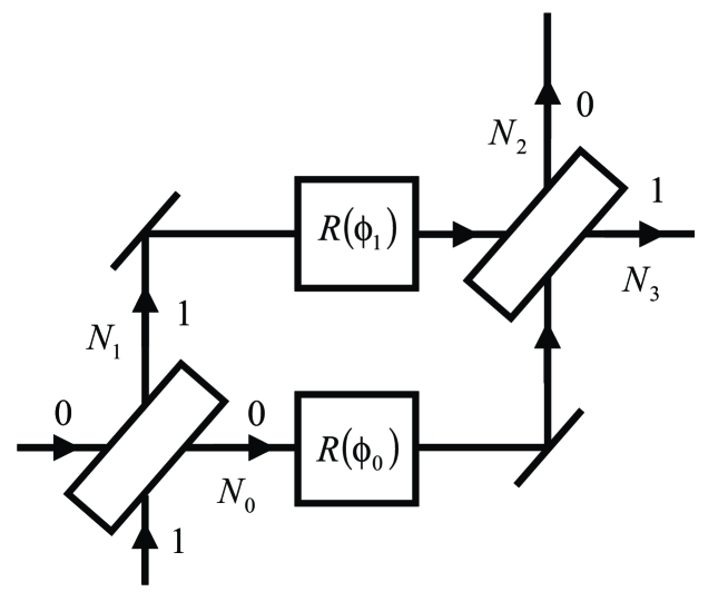
Figure 3: Diagram of a DLM network that simulates a single-photon Mach-Zehnder interferometer on an event-by-event basis [11]. The DLM network consists of two BS devices (see Fig. 1) and two passive devices $R(\phi_{0})$ and $R(\phi_{1})$ (see Eq. (5)) that perform plane rotations by $\phi_{0}$ and $\phi_{1}$, respectively. The number of events $N_{i}$ in channel $i=0,\ldots,3$ is proportional to the probability for finding a photon on the corresponding arm of the interferometer.

3 Single-Photon Beam Splitter

In quantum theory, [10] the presence of photons in the input modes 0 or 1 of a beam splitter is represented by the complex-valued amplitudes ($a_{0},a_{1}$) [14, 2, 15]. According to quantum theory, the complex-valued amplitudes ($b_{0},b_{1}$) of the photons in the output channels 0 and 1 of a beam splitter are given by [14, 2, 15]

$$\left(\begin{array}[]{c}b_{0}\\ b_{1}\end{array}\right)=\frac{1}{\sqrt{2}}\left(\begin{array}[]{cc}1&i\\ i&1\end{array}\right)\left(\begin{array}[]{c}a_{0}\\ a_{1}\end{array}\right),$$ (18)

Writing $a_{0}=\sqrt{p_{0}}e^{i\psi_{0}}$ and $a_{1}=\sqrt{1-p_{0}}e^{i\psi_{1}}$, the probability to observe a photon in output channel 0 (1) is given by

$$|b_{0}|^{2} = \frac{1+\sqrt{p_{0}(1-p_{0})}\sin(\psi_{0}-\psi_{1})}{2},$$ (19)

$$|b_{1}|^{2} = \frac{1-\sqrt{p_{0}(1-p_{0})}\sin(\psi_{0}-\psi_{1})}{2}.$$ (20)

Here $\psi_{0}$ and $\psi_{1}$ represent the phases of the photons. In a quantum theoretical description, this phase is proportional to the length of the optical path that the photons have travelled before they enter the beam splitter [14, 2, 15].

We now show that the DLM-network shown in Fig.1 behaves as if it is a single-photon beam splitter. This network receives events at one of the two input channels. There is a one-to-one relation between each input channel and the corresponding input mode of the quantum mechanical description. Each input event carries information in the form of a two-dimensional unit vector. Either input channel 0 receives $(y_{0},y_{1})=(\cos\psi_{0},\sin\psi_{0})$ or input channel 1 receives $(y_{2},y_{3})=(\cos\psi_{1},\sin\psi_{1})$. In terms of the single-photon experiments of Grangier et al. [2], an event corresponds to the arrival of a photon at channel 0 (1) with phase $\psi_{0}$ ($\psi_{1}$) of the beam splitter (see Fig. 1).

The input message is fed into the DLM-network described in Section 2. The purpose of DLM 1 is to transform the information contained in two-dimensional input vectors (of which only one is present for any given input event), into a four-dimensional unit vector. The internal vector ${\bf x}$ of DLM 1 learns about the amplitudes ($a_{0},a_{1}$): In the stationary regime we have

$$x_{0} \approx \sqrt{p_{0}}\cos{\psi_{0}},$$

$$x_{1} \approx \sqrt{p_{0}}\sin{\psi_{0}},$$

$$x_{2} \approx \sqrt{1-p_{0}}\cos{\psi_{1}},$$

$$x_{3} \approx \sqrt{1-p_{0}}\sin{\psi_{1}}.$$ (21)

The four-dimensional internal vector of this device is split into two groups of two-dimensional vectors $(x_{0},x_{3})$ and $(x_{2},x_{1})$ and each of these two-dimensional vectors is rotated by $45^{\circ}$. Put differently, the four-dimensional vector is rotated once in the (1,4)-plane about $45^{\circ}$ and once in the (3,2) plane about $45^{\circ}$. The order of the rotations is irrelevant. Physically, this transformation corresponds to the reflection of the photons by $45^{\circ}$ at the beam splitter. The resulting four-dimensional vector is then sent to the input of DLM 2. The internal vector ${\bf z}$ of DLM 2 learns about the amplitudes ($b_{0},b_{1}$): In the stationary regime we have

$$z_{0} \approx \sqrt{p_{0}}\cos{\psi_{0}}-\sqrt{1-p_{0}}\sin{\psi_{1}},$$

$$z_{1} \approx \sqrt{p_{0}}\sin{\psi_{0}}+\sqrt{1-p_{0}}\cos{\psi_{1}},$$

$$z_{2} \approx \sqrt{1-p_{0}}\cos{\psi_{1}}-\sqrt{p_{0}}\cos{\psi_{0}},$$

$$z_{3} \approx \sqrt{1-p_{0}}\sin{\psi_{1}}+\sqrt{p_{0}}\cos{\psi_{0}}$$ (22)

DLM 2 sends $(z_{0},z_{1})$ through output channel 0 if it used rule $m=1,2,3,4$ (see Eq. (7)) to update its internal state. Otherwise it sends $(z_{2},z_{3})$ through output channel 1.

In Fig. 2 we present results of discrete-event simulations using the DLM network depicted in Fig. 1. We denote the number of 0 (1) events by $N_{0}$ ($N_{1}$) and the total number of events by $N=N_{0}+N_{1}$. The correspondence with the quantum system is clear: the probability for a 0 event is given by $|b_{0}|^{2}\approx N_{0}/N$, $y_{0}^{\prime}=\hbox{Re }b_{0}/|b_{0}|$ and $y_{1}^{\prime}=\hbox{Im }b_{0}/|b_{0}|$. The probability for a 1 event is $|b_{1}|^{2}\approx N_{1}/N$, $y_{2}^{\prime}=\hbox{Re }b_{1}/|b_{1}|$ and $y_{3}^{\prime}=\hbox{Im }b_{1}/|b_{1}|$. Before the simulation starts, the internal vectors of the DLMs are given a random value (on the unit sphere). Each data point represents 10000 events. All these simulations were carried out with $\alpha=0.99$. The simulation procedure itself consists of four steps:

1. Use two uniform random numbers in the range $[0,360]$ to generate $\psi_{0}$ and $\psi_{1}$.

2. For fixed values of $\psi_{0}$ and $\psi_{1}$, generate 10000 input events. Input channel 0 receives $(y_{0},y_{1})=(\cos\psi_{0},\sin\psi_{0})$ with probability $p_{0}$. Input channel 1 receives $(y_{2},y_{3})=(\cos\psi_{1},\sin\psi_{1})$ with probability $p_{1}=1-p_{0}$.

3. Count the number of output events $N_{0}$ ($N_{1}$) in channel 0 (1), see Fig. 1.

4. Repeat steps 1 to 3. For each pair ($\psi_{0}$,$\psi_{1}$), store the results for $N_{0}$ ($N_{1}$).

Plotting $N_{0}/(N_{0}+N_{1})$ and $|b_{0}|^{2}$ as a function of $\phi=\psi_{0}-\psi_{1}$ yields the results shown in Fig. 2. Actually, there is no need to use random numbers to generate $\psi_{0}$ and $\psi_{1}$. In Fig. 2, we only used this random process to show that the order in which we pick $\psi_{0}$ and $\psi_{1}$ is irrelevant. Random processes enter in the procedure to generate the input data only. The DLM network processes the events sequentially and deterministically. From Fig. 2 it is clear that the output of the deterministic DLM-based beam splitter reproduces the probability distributions as obtained from quantum theory [10].

Figure 4: Simulation results for the DLM-network shown in Fig. 3. Markers give the simulation results for the normalized intensities as a function of $\phi_{0}$. Open squares: $N_{0}/(N_{0}+N_{1})$; Solid squares: $N_{2}/(N_{2}+N_{3})$ for $\phi_{1}=0$; Open circles: $N_{2}/(N_{2}+N_{3})$ for $\phi_{1}=30^{\circ}$; Bullets: $N_{2}/(N_{2}+N_{3})$ for $\phi_{1}=240^{\circ}$; Asterisks: $N_{3}/(N_{2}+N_{3})$ for $\phi_{1}=0$; Solid triangles: $N_{3}/(N_{2}+N_{3})$ for $\phi_{1}=300^{\circ}$. Lines represent the results of quantum theory.

4 Mach-Zehnder Interferometer

In quantum physics [10], single-photon experiments with one beam splitter provide direct evidence for the particle-like behavior of photons [2, 5]. The wave mechanical character appears when one performs single-particle interference experiments. We now describe a DLM network that displays the same interference patterns as those observed in single-photon Mach-Zehnder interferometer experiments [2]. The schematic layout of the DLM network is shown in Fig. 3. The network described in Section 3 is used for the beam splitters. The phase shift is taken care of by the devices $R(\phi_{0})$ and $R(\phi_{1})$ (that do not contain DLMs) that perform plane rotations by $\phi_{0}$ and $\phi_{1}$ (see Eq. (5), respectively. Clearly there is a one-to-one correspondence between the components of the DLM network and the elements of a physical Mach-Zehnder interferometer [13, 2].

According to quantum theory [10], the amplitudes ($b_{0},b_{1})$ of the photons in the output modes 0 ($N_{2}$) and 1 ($N_{3}$) of the Mach-Zehnder interferometer are given by [14, 2, 15]

$$\left(\begin{array}[]{c}b_{0}\\ b_{1}\end{array}\right)=U\left(\begin{array}[]{c}a_{0}\\ a_{1}\end{array}\right),$$ (27)

where

$$U=\frac{1}{2}\left(\begin{array}[]{cc}1&i\\ i&1\end{array}\right)\left(\begin{array}[]{cc}e^{i\phi_{0}}&0\\ 0&e^{i\phi_{1}}\end{array}\right)\left(\begin{array}[]{cc}1&i\\ i&1\end{array}\right),$$ (34)

and $a_{0}$ ($a_{1})$ denotes the amplitude of the photons in the input channel 0 (1). Note that in experiments it is impossible to simultaneously measure ($N_{0}/(N_{0}+N_{1})$, $N_{1}/(N_{0}+N_{1})$) and ($N_{2}/(N_{0}+N_{1})$, $N_{3}/(N_{0}+N_{1})$): Photon detectors operate by absorbing photons.

In experiment [13, 2], there are no photons in input channel 1 of the first beam splitter, that is $a_{1}=0$. From Eq. (27), we see that the phase of the wave function describing the photons in input channel 0 of the first beam splitter is irrelevant. However, as the photons leave the first beam splitter the relation between their phases is fixed. This relation can be changed through the optical path length for reaching the second beam splitter. A change of the optical path length in channel 0 (1) results in a phase shift by $\phi_{0}$ ($\phi_{1}$). If $a_{1}=0$, the output amplitudes of the Mach-Zehnder interferometer are given by

$$b_{0} = a_{0}|a_{0}|^{-1}e^{i(\phi_{0}+\phi_{1})/2}\sin\frac{\phi_{0}-\phi_{1}}{2},$$

$$b_{1} = a_{0}|a_{0}|^{-1}e^{i(\phi_{0}+\phi_{1})/2}\cos\frac{\phi_{0}-\phi_{1}}{2},$$ (35)

from which we see that the probabilities $|b_{0}|^{2}$ and $|b_{1}|^{2}$ depend on $\phi=\phi_{0}-\phi_{1}$ only.

In Fig. 4 we present a representative selection of simulation results for the Mach-Zehnder interferometer built from DLMs. We assume that input channel 0 receives $(y_{0},y_{1})=(\cos\psi_{0},\sin\psi_{0})$ with probability one and that input channel 1 receives no events. This corresponds to $(a_{0},a_{1})=(\cos\psi_{0}+i\sin\psi_{0},0)$ in Eq. (27). We use uniform random numbers to determine $\psi_{0}$. As in the case of the beam splitter, we only use this random process to show that the order in which we pick $\psi_{0}$ is irrelevant. In all these simulations $\alpha=0.99$. The data points are the simulation results for the normalized intensity $N_{i}/(N_{0}+N_{1})$ for i=0,2,3 as a function of $\phi=\phi_{0}-\phi_{1}$. Each data point represents 10000 events ($N_{0}+N_{1}=N_{2}+N_{3}=10000$). Initially the rotation angle $\phi_{0}=0$ and after each set of 10000 events, $\phi_{0}$ is increased by $10^{\circ}$. Lines represent the corresponding results of quantum theory [10]. From Fig. 4 it is clear that the deterministic, event-based DLM network generates events with frequencies that are in excellent agreement with quantum theory.

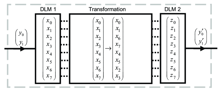
Figure 5: Diagram of a DLM-based processor that simulates a CNOT gate on an event-by-event basis.

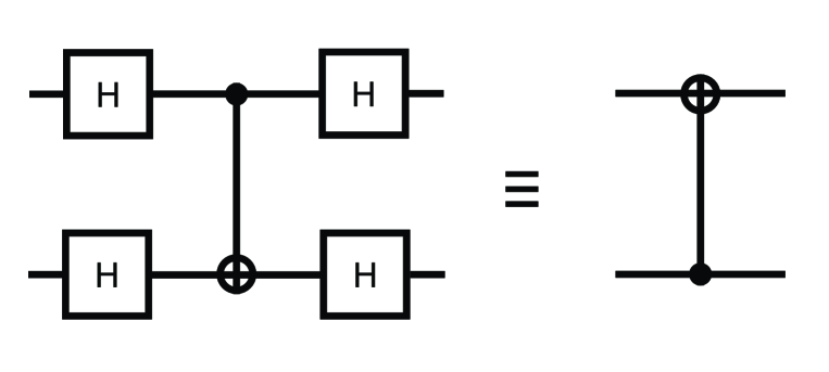
Figure 6: Quantum circuit representation of two equivalent CNOT operations. The dot and the cross on the line denote the control and target qubit, respectively. The square boxes labeled $H$ represent Hadamard gates.

5 Universal quantum computation

It has been shown that an arbitrary unitary operation, that is, the time evolution of a quantum system, can be written as a sequence of single-qubit operations and the controlled-NOT (CNOT) operation on two qubits [16, 17]. Therefore, in principle, single-qubit operations and the CNOT operation are sufficient to construct a universal quantum computer or to simulate any quantum system [17]. In this section, we present results of event-based simulations of single qubit operations and a two-qubit quantum circuit containing the CNOT operation to illustrate that DLM-based networks can be used to simulate universal quantum computers.

The state vector of a two-qubit system can be written as [14, 7, 17]

$$|\Phi\rangle = a_{0}|0\rangle_{1}|0\rangle_{2}+a_{1}|1\rangle_{1}|0\rangle_{2}+a_{2}|0\rangle_{1}|1\rangle_{2}$$ (36)

$$+a_{3}|1\rangle_{1}|1\rangle_{2}$$

$$= a_{0}|00\rangle+a_{1}|01\rangle+a_{2}|10\rangle+a_{3}|11\rangle$$

$$= a_{0}|0\rangle+a_{1}|1\rangle+a_{2}|2\rangle+a_{3}|3\rangle,$$

where $a_{0},\ldots a_{3}$ are the amplitudes of the four different states and $|0\rangle_{i}$ and $|1\rangle_{i}$ represent the 0 and 1 state of the $i$-th qubit, respectively. For convenvience, in the last line of Eq.(36), we represent the basis states of the two-qubit system in decimal notation, that is $|00\rangle=|0\rangle$, $|01\rangle=|1\rangle$, $|10\rangle=|2\rangle$, and $|11\rangle=|3\rangle$ [17].

Table 1: Simulation results for the DLM-network shown in Fig. 6, demonstrating that the network reproduces the results of the corresponding quantum circuit, that is, a CNOT operation in which qubit 2 is the control qubit and qubit 1 is the target qubit [17]. The first half of the events are discarded in the calculation of the frequencies $f_{i}$ for observing an output event of type $i=0,1,2,3$. For 200 events or more, the difference between the event-based simulation results and the corresponding quantum mechanical probabilities is less than 1%.

Processor	Number of events	Qubit 1	Qubit 2	$f_{0}$	$f_{1}$	$f_{2}$	$f_{3}$
Deterministic	100	0	0	$0.98$	$0.00$	$0.00$	$0.02$
Deterministic	100	1	0	$0.20$	$0.74$	$0.01$	$0.04$
Deterministic	100	0	1	$0.16$	$0.04$	$0.00$	$0.80$
Deterministic	100	1	1	$0.16$	$0.04$	$0.72$	$0.08$
Deterministic	200	0	0	$1.00$	$0.00$	$0.00$	$0.00$
Deterministic	200	1	0	$0.00$	$1.00$	$0.00$	$0.00$
Deterministic	200	0	1	$0.00$	$0.00$	$0.00$	$1.00$
Deterministic	200	1	1	$0.01$	$0.00$	$0.99$	$0.00$
Stochastic	2000	0	0	$0.965$	$0.015$	$0.010$	$0.010$
Stochastic	2000	1	0	$0.007$	$0.970$	$0.012$	$0.011$
Stochastic	2000	0	1	$0.010$	$0.008$	$0.016$	$0.966$
Stochastic	2000	1	1	$0.005$	$0.016$	$0.963$	$0.016$

Table 2: Same as in Table  1 except that the control parameter $\alpha=0.999$ instead of $\alpha=0.99$ and that ten times as many event were generated. The results for the deterministic simulations are exact within three-digit accuracy and have therefore been omitted.

Processor	Number of events	Qubit 1	Qubit 2	$f_{0}$	$f_{1}$	$f_{2}$	$f_{3}$
Stochastic	20000	0	0	$0.995$	$0.003$	$0.001$	$0.002$
Stochastic	20000	1	0	$0.002$	$0.995$	$0.003$	$0.001$
Stochastic	20000	0	1	$0.002$	$0.001$	$0.002$	$0.995$
Stochastic	20000	1	1	$0.001$	$0.002$	$0.997$	$0.001$

5.1 CNOT gate

By definition, the CNOT gate flips the target qubit if the control qubit is in the state $|1\rangle$ [17]. If we take qubit 1 (that is, the least significant bit in the binary notation of an integer) as the control qubit, we have

$${\mathop{\hbox{CNOT}}}|\Phi\rangle = a_{0}|0\rangle_{1}|0\rangle_{2}+a_{3}|1\rangle_{1}|0\rangle_{2}+a_{2}|0\rangle_{1}|1\rangle_{2}$$ (37)

$$+a_{1}|1\rangle_{1}|1\rangle_{2}$$

$$= a_{0}|00\rangle+a_{3}|01\rangle+a_{2}|10\rangle+a_{1}|11\rangle$$

$$= a_{0}|0\rangle+a_{3}|1\rangle+a_{2}|2\rangle+a_{1}|3\rangle.$$

The schematic diagram of the DLM-network that performs the CNOT operation on an event-by-event (particle-by-particle) basis is shown in Fig. 5. Conceptually the structure of this network is the same as in the case of the Mach-Zehnder interferometer. As input to the DLM-network we now have four (0,1,2 or 3) instead of two different types of events. Each event carries a message consisting of two real numbers ${\bf y}=(y_{0},y_{1})$, corresponding to the quantum mechanical amplitudes $a_{0},\ldots a_{3}$. The internal state of each DLM is represented by a unit vector of eight real numbers ${\bf x}=(x_{0},\dots,x_{7})$ and there are $16$ candidate update rules ($\{j=0,\ldots 7;s_{j}=\pm 1\}$, see Eq.(6)) to choose from. The rule that is actually used is determined by minimizing the cost function given by Eq.(7). The transformation stage is extremely simple: According to Eq.(37), all it has to do is swap the two pairs of elements ($x_{2}$,$x_{3}$) and ($x_{6}$,$x_{7}$).

Instead of presenting results that show that a DLM-processor correctly simulates the CNOT operation on an event-by-event basis, we consider the more complicated network of four Hadamard gates and one CNOT gate shown in Fig. 6 [17]. Quantum mechanically, this network acts as a CNOT gate in which the role of control- and target qubit have been interchanged [17]. For the corresponding DLM-network to work properly it is essential that the event-based simulation mimics the quantum interference (generated by the Hadamard gates) correctly.

5.2 Hadamard operation

The Hadamard operation $H$ is the single-qubit operation defined by [17]

$$H\equiv\frac{1}{\sqrt{2}}\left(\begin{array}[]{cc}\phantom{-}1&\phantom{-}1\\ \phantom{-}1&-1\end{array}\right).$$ (38)

Disregarding phase factors, it performs the same operation as a beam splitter.

The structure of a DLM-processor that performs a general single-qubit operation is identical to the one shown in Fig. 1. The only difference is in the transformation stage. To implement the Hadamard operation, we use the transformation matrix $T$ (see Fig. 1)

$$\frac{1}{\sqrt{2}}\left(\begin{array}[]{cccc}\phantom{-}1&\phantom{-}0&\phantom{-}1&\phantom{-}0\\ \phantom{-}0&\phantom{-}1&\phantom{-}0&\phantom{-}1\\ \phantom{-}1&\phantom{-}0&-1&\phantom{-}0\\ \phantom{-}0&\phantom{-}1&\phantom{-}0&-1\\ \end{array}\right).$$ (39)

5.3 Simulation results

In Table 1, we present simulation results for the DLM-network shown in Fig. 6. Before the first simulation starts we use uniform random numbers to initialize the internal vectors of the DLMs (ten vectors in total). All these simulations were carried out with $\alpha=0.99$. From Table 1, it is clear that, also for a modest number of events, the network reproduces the results of the corresponding quantum circuit, that is, a CNOT operation in which qubit 2 is the control qubit and qubit 1 is the target qubit [17].

As an illustration of the use of SLMs, we replace all the DLM 2’s by SLMs in the DLM implementation of the circuit shown in Fig. 6 and repeat the simulations. From Tables 1 and  2, we conclude that the randomized version generates the correct results but significantly more events are needed to achieve similar accuracy as in the fully deterministic simulation.

5.4 Technical note

All simulations that we presented in this section have been performed for $\alpha=0.99$. From the description of the learning process it is clear that $\alpha$ controls the rate of learning or, equivalently, the rate at which learned information can be forgotten. Furthermore it is evident that the difference between a constant input to a DLM and the learned value of its internal variable cannot be smaller than $1-\alpha$. In other words, $\alpha$ also limits the precision with which the internal variable can represent a sequence of constant input values. On the other hand, the number of events has to balance the rate at which the DLM can forget a learned input value. The smaller $1-\alpha$ is, the larger the number of events has to be for the DLM to adapt to changes in the input data.

We use the example of this section to illustrate the effect of changing $\alpha$ and the total number of events $N$. In Table 2 we show the results of repeating the procedure used to obtain the data shown in Table 1 but instead of $\alpha=0.99$ we used $\alpha=0.999$ and adjusted the number of events accordingly. As expected, the difference between the simulation data and the results of quantum theory decreases if $1-\alpha$ decreases and the number of events increases accordingly. Comparing Table 1 with Table 2 it is clear that the decrease of this difference is roughly proportional to the inverse of the square root of the number of events.

6 Discussion

We have proposed a new procedure to construct algorithms that can be used to simulate quantum processes without solving the Schrödinger equation. There is a one-to-one correspondence between the components of the network and the processing units and the physical parts of the experimental setup. Furthermore, only simple geometry is used to construct the simulation algorithm. In this sense, the simulation approach we propose satisfies Einstein’s criteria of realism and causality [5].

An analogy may be helpful to understand the conceptual difference between the conventional description of quantum theory and the event-based approach proposed in this paper. It is well known that an ensemble of simple, symmetric random walks may be approximated by a diffusion equation (for vanishing lattice spacing and time step). Also here we have two options. If we are interested in individual events, we have no other choice than to simulate the discrete random walk. However, if we want to study the behavior of many random walkers, it is computationally much more efficient to solve the corresponding diffusion problem. The latter describes the outcome of (infinitly) many individual events but does not provide information about individual events. The random walk is the fundamental mechanism that gives rise to diffusion behavior. In this sense, the DLMs described in this paper may be regarded as building blocks for a dynamic, deterministic, local and causal system that generates individual events in such a manner that the collective behavior of these events is described by quantum theory.

It may be of interest to compare our approach with stochastic wavefunction methods [18, 19, 20, 21, 22, 23, 24, 25, 26, 27, 28, 29, 30, 31, 32, 33]. Instead of solving the equation of motion of the density matrix, these methods solve stochastic differential equations for an ensemble of independent realizations of pure states. Typically, these methods are used to study open quantum systems in which a small number of degrees of freedom is coupled to a large reservoir. An attempt to use a variant of the stochastic wavefunction method to perform an event-by-event study of photon emission was reported in Ref. [30]. In stochastic wavefunction methods, the wave function evolves in time according to the time-dependent Schrödinger equation. An uncorrelated random process interrupts this evolution to project the wave function (that is, make a quantum jump) onto another normalized state. This evolution of the wave function is similar to the change of the internal state of a SLM if we consider one isolated event that is processed by the transformation stage $T$ and a SLM (see Fig. 1). However, as a SLM is capable of learning from previous events, the process of generating output events is non-Markovian, this similarity being very superficial. The fundamental difference between the two approaches can also be seen as follows. In the stochastic wavefunction method, we can calculate the time evolution of each member of the ensemble in parallel, at least in principle. In the DLM-approach, this is impossible: To exhibit quantum mechanical behavior, it is imperative that the DLM-network processes events in a sequential manner. In the fully deterministic DLM-approach (that is, without the randomizing feature of the SLM), there is no stochastic process at all. Therefore, there also is no relation between the stochastic wavefunction method and the deterministic, machine-learning approach discussed in this paper.

In conclusion, we have shown that single-particle quantum interference and quantum computers can be simulated on an event-by-event basis using local and causal processes, without the need of concepts such as wave functions or particle-wave duality.

References

- [1] D.P. Landau and K. Binder, A Guide to Monte Carlo Simulation in Statistical Physics, Cambridge University Press, Cambridge, (2000).
- [2] P. Grangier, R. Roger, and A. Aspect, Europhys. Lett. 1 (1986) 173.
- [3] A. Tonomura, The Quantum World Unveiled by Electron Waves, World Scientific, Singapore (1998).
- [4] In this paper we disregard limitations of real experiments such as detector efficiency, imperfection of the source, biprism etc.
- [5] D. Home, Conceptual Foundations of Quantum Physics, Plenum Press, New York (1997).
- [6] R.P. Feynman, R.B. Leighton, M. Sands, The Feynman lectures on Physics, Vol. 3, Addison-Wesley, Reading MA, (1996).
- [7] L.E. Ballentine, Quantum Mechanics: A Modern Development, World Scientific, Singapore (2003).
- [8] R. Penrose, The Emperor’s New Mind, Oxford University Press, Oxford (1990).
- [9] N.G. Van Kampen, Physica A 153 (1988) 97.
- [10] We make a distinction between quantum theory and quantum physics. We use the term quantum theory when we refer to the mathematical formalism, that is, the postulates of quantum mechanics (with or without the wave function collapse postulate) [7] and the rules (algorithms) to compute the wave function. We use the term quantum physics for microscopic, experimentally observable phenomena that do not find an explanation within the mathematical framework of classical mechanics.
- [11] An interactive program that performs the event-based simulations of a beam splitter, one Mach-Zehnder interferometer, and two chained Mach-Zehnder interferometers can be found at http://www.compphys.net/dlm
- [12] K. De Raedt, H. De Raedt, and K. Michielsen, Deterministic event-based simulation of quantum interference, arXiv: quant-ph/0409213.
- [13] M. Born and E. Wolf, Principles of Optics, Pergamon, Oxford (1964).
- [14] G. Baym, Lectures on Quantum Mechanics, W.A. Benjamin, Reading MA (1974).
- [15] J.G. Rarity and P.R. Tapster, Phil. Trans. R. Soc. Lond. A 355 (1997) 2267.
- [16] D.P. DiVincenzo, Phys. Rev. A 51 (1995) 1015.
- [17] M. Nielsen and I. Chuang, Quantum Computation and Quantum Information, Cambridge University Press, Cambridge (2000).
- [18] N. Gisin, Phys. Rev. Lett. 52 (1984) 1657.
- [19] J. Dalibard, Y. Castin, and K. Mølmer, Phys. Rev. Lett. 68 (1992) 580.
- [20] R. Dum, P. Zoller, and H. Ritsch, Phys. Rev. A 45 (1992) 4879.
- [21] C.W. Gardiner, A.S. Parkins, and P. Zoller, Phys. Rev. A 46 (1992) 4363.
- [22] K. Mølmer, Y. Castin, and J. Dalibard, J. Opt. Soc. Am. B 10 (1993) 524.
- [23] B.M. Garraway and P.L. Knight, Phys. Rev. A 49 (1994) 1266.
- [24] H.P. Breuer and F. Petruccione, Phys. Rev. E 51 (1995) 4041.
- [25] H.P. Breuer and F. Petruccione, Phys. Rev. Lett. 74 (1995) 3788.
- [26] H. Ezaki, S. Miyashita, and E. Hanamura, Phys. Lett. A 203 (1995) 403.
- [27] H.P. Breuer and F. Petruccione, Phys. Rev. E 52 (1995) 428.
- [28] H.P. Breuer and F. Petruccione, J. Phys. A 29 (1996) 7837.
- [29] T.A. Brun, Phys. Rev. Lett. 78 (1997) 1833.
- [30] S. Miyashita, H. Ezaki, and E. Hanamura, Phys. Rev. A 57 (1998) 2046.
- [31] H.P. Breuer, B. Kappler and F. Petruccione, Phys. Rev. A 59 (1999) 1633.
- [32] H.P. Breuer, Phys. Rev. A 68 (2003) 032105.
- [33] H.P. Breuer, Phys. Rev. A 69 (2004) 022115.