Self-induced decoherence approach: Strong limitations on its validity in a simple spin bath model and on its general physical relevance

Abstract

The “self-induced decoherence” (SID) approach suggests that (1) the expectation value of any observable becomes diagonal in the eigenstates of the total Hamiltonian for systems endowed with a continuous energy spectrum, and that (2) this process can be interpreted as decoherence. We evaluate the first claim in the context of a simple spin bath model. We find that even for large environments, corresponding to an approximately continuous energy spectrum, diagonalization of the expectation value of random observables does in general not occur. We explain this result and conjecture that SID is likely to fail also in other systems composed of discrete subsystems. Regarding the second claim, we emphasize that SID does not describe a physically meaningful decoherence process for individual measurements, but only involves destructive interference that occurs collectively within an ensemble of presupposed “values” of measurements. This leads us to question the relevance of SID for treating observed decoherence effects.

I Introduction

In a series of papers Castagnino and Lombardi (2005, 2004); Castagnino and Gadella (2003); Castagnino and Lombardi (2003); Castagnino and Ordóñez (2001); Castagnino et al. (2001); Castagnino and Laura (2000a, b, c); Laura et al. (1999); Castagnino (1999); Laura and Castagnino (1998a, b); Castagnino and Laura (1997), the authors claim to present a “new approach to decoherence” Castagnino and Lombardi (2004), termed “self-induced decoherence” (SID). Their main assertion is that, for systems endowed with a continuous energy spectrum, the expectation value of an observable will become diagonal in the eigenbasis of the Hamiltonian of the system, and that this effect can be viewed as decoherence.

The basic idea underlying SID goes back to well-known arguments in the context of quantum measurement and the theory of irreversible processes Pauli (1928); van Kampen (1954); Daneri et al. (1962); Hepp (1972); Peres (1980); van Hove (1959, 1955, 1957). It rests on the observation that a superposition of a large number of terms with random phases in the expression for the expectation value of a typical observable, or for the matrix elements of the density operator, leads to destructive interference. The phase differences are either due to a random-phase assumption Pauli (1928), or, as in SID, are created dynamically through the time evolution factor $e^{iEt/\hbar}$ associated with each energy eigenstate in the superposition. These destructive interference effects are then responsible for the diagonalization of the expectation value in the energy eigenbasis as described by SID.

However, this process differs strongly from the mechanism of environment-induced decoherence (EID) Joos et al. (2003); Zurek (1981, 1982, 1993, 1998, 2003); Schlosshauer (2004); Zeh (1970, 1973). EID understands decoherence as the practically irreversible dislocalization of local phase relations between environment-selected preferred basis states due to entanglement with an environment. The approximate diagonality of the expectation value of local observables expressed in the preferred basis is only a formal phenomenological consequence of the relative states of the environment becoming rapidly orthogonal during the decoherence process. The fact that SID does not require an explicit environment interacting with the system motivated the term “self-induced” and was suggested Castagnino and Lombardi (2004) to circumvent the question of a proper interpretation of the concept of “observational ignorance of the environment” in EID d’Espagnat (1988); Joos et al. (2003); Zurek (1998); Schlosshauer (2004).

This paper pursues two main goals. First, after formalizing the basic idea of SID (Sec. II), we shall discuss the question to what extent SID can claim to describe a physically relevant decoherence process (Sec. III). In particular, we will argue that, contrary to the claim of its proponents Castagnino and Lombardi (2004), SID does not constitute a “new viewpoint” on decoherence in the usual definition of EID. Second, we shall study whether diagonalization of the expectation value of random observables in the energy eigenbasis is obtained in the context of an explicit spin bath model (Sec. IV). Deliberately, we have chosen a discrete model to investigate the required degree of “quasicontinuity” for SID to work as claimed. To anticipate, we find that even for bath sizes large compared to what is typically considered in EID, no general decay of off-diagonal terms is found, unless both the observable and the initial state of the bath are appropriately restricted. We explain and discuss this result in Sec. V, and present our conclusions in Sec. VI.

II Self-induced decoherence

The basic formalism of SID as developed in Refs. Castagnino and Lombardi (2004); Castagnino and Gadella (2003); Castagnino and Lombardi (2003); Castagnino and Ordóñez (2001); Castagnino et al. (2001); Castagnino and Laura (2000a, b, c); Laura et al. (1999); Castagnino (1999); Laura and Castagnino (1998a, b); Castagnino and Laura (1997) considers an arbitrary observable

$$\widehat{O}=\int dE\int dE^{\prime}\,\widetilde{O}(E,E^{\prime})|{E\rangle}{\langle E^{\prime}}|,$$ (1)

expanded in the eigenstates $|{E\rangle}$ of the Hamiltonian $\widehat{H}=\int dE\,E|{E\rangle}{\langle E}|$ with continuous spectrum. In the general treatment, only observables with

$$\widetilde{O}(E,E^{\prime})=O(E)\delta(E-E^{\prime})+O(E,E^{\prime})$$ (2)

are considered, where $O(E)$ and the $O(E,E^{\prime})$ are assumed to be regular functions. The time evolution of the expectation value $\langle\widehat{O}\rangle_{\Psi(t)}$ of $\widehat{O}$ in the pure state $|{\Psi(t)\rangle}=e^{-iHt}|{\Psi_{0}\rangle}=\int dE\,e^{-iEt}{\langle E}|{\Psi_{0}\rangle}|{E\rangle}$ (setting $\hbar=1$) is then given by

$$\langle\widehat{O}\rangle_{\Psi(t)}=\int dE\,O(E)|{\langle E}|{\Psi_{0}\rangle}|^{2}\\ \,\,+\int dE\int dE^{\prime}\,e^{-i\Delta Et}O(E,E^{\prime}){\langle E}|{\Psi_{0}\rangle}{\langle\Psi_{0}}|{E^{\prime}\rangle},$$ (3)

where $\Delta E=E-E^{\prime}$. For large $t$, the phase factor $e^{-i\Delta Et}$ fluctuates rapidly with $\Delta E$, which leads to destructive interference in the double integral if the multiplying function $f(E,E^{\prime})\equiv O(E,E^{\prime}){\langle E}|{\Psi_{0}\rangle}{\langle\Psi_{0}}|{E^{\prime}\rangle}$ varies comparably slowly. To formalize this argument, SID employs the Riemann-Lebesgue theorem Reed and Simon (1975), which prescribes that

$$\lim_{t\rightarrow\infty}\int dz\,g(z)e^{izt}=0,$$ (4)

if $g(z)$ is a regular function and $L^{1}$ integrable (i.e., $\int dz\,|g(z)|<\infty$). Provided these conditions are satisfied by $f(E,E^{\prime})$, it is concluded that

$$\langle\widehat{O}\rangle_{\Psi(t)}\longrightarrow\int dE\,O(E)|{\langle E}|{\Psi_{0}\rangle}|^{2},$$ (5)

for large $t$. Thus, the off-diagonal terms $E\not=E^{\prime}$ have collectively disappeared, which in SID is interpreted as “decoherence in the expectation value.” Formally, the SID program introduces a “diagonal-equivalent” density matrix $\rho_{d}$,

$$\rho_{d}=\int dE\,|{\langle E}|{\Psi_{0}\rangle}|^{2}|{E\rangle}{\langle E}|,$$ (6)

which satisfies $\langle\widehat{O}\rangle_{\rho_{d}}\equiv\lim_{t\rightarrow\infty}\langle\widehat{O}\rangle_{\rho(t)}$. Note that $\rho_{d}$ is only a formal equivalent and is not obtained through any dynamical process. Also, expectation values of a nonexhaustive set of observables [see Eq. (2)] do not uniquely determine the density matrix. Therefore, one must not derive any conclusions about the possibility for certain states of the system from $\rho_{d}$.

To summarize, the main result Eq. (5) has been obtained from two key assumptions: (1) The energy spectrum of the system is continuous; and (2) the coefficients used in expanding the initial state and the observable in the energy eigenbasis form regular (and integrable) functions of the energy variable.

The first requirement of a continuous energy spectrum can be viewed as an implicit inclusion of an internal “environment” with an infinite number of degrees of freedom. However, any realistic physical system is of finite size, and therefore the energy spacing will be discrete. An approximate suppression of off-diagonal terms as given by Eq. (5) should therefore occur also for quasicontinuous energy spectra, i.e., for small but discrete energy spacings.

The regularity assumption (2) is crucial, since it ensures that the phase factors $e^{i\Delta Et}$ are able to lead to the required destructive interference of the expansion coefficients for large times. However, especially in the realistic case of systems of finite size where the expansion coefficients will be a finite set of discrete values, this condition will not hold. It is therefore important to understand the physical meaning and the consequences of a violation of this assumption.

Note also that the strict mathematical limit $t\rightarrow\infty$ employed in the Riemann-Lebesgue theorem, Eq. (4), is not physically meaningful, and approximate suppression must therefore occur already over finite time scales, as indicated in Eq. (5). Also, for the realistic case of only quasicontinuous (i.e., essentially discrete) energy spectra, no conclusions about an “irreversibility” of the decay should be derived from the limit $t\rightarrow\infty$ (as it is done, for example, in Ref. (Castagnino and Lombardi, 2004, p. 88)), since the off-diagonal terms will return to their initial values within a finite recurrence time scale.

The issues outlined above will be illustrated and investigated in the context of a particular model system in Sec. IV.

III Does SID describe decoherence?

Despite the fact that SID and EID share the term “decoherence” in their name, we shall demonstrate in this section that their foundations, scope, and physical implications are fundamentally different. Keeping these differences in mind is very important for a proper interpretation of the study of the bath model described in the following Sec. IV.

As already briefly outlined in the Introduction, the standard approach of environmental decoherence Joos et al. (2003); Zurek (1981, 1982, 1993, 1998, 2003); Schlosshauer (2004); Zeh (1970, 1973) describes the consequences of the ubiquitous interaction of any system with its environment. This leads to entanglement between the system and the environment and singles out a preferred basis of the system that is dynamically determined by the Hamiltonian governing the interaction. The relative environmental states associated with these preferred states rapidly approach orthogonality (i.e., macroscopic distinguishability). Phase relations between the preferred states that were initially associated with the system alone are now “dislocalized” into the system-environment combination due to the entanglement, which constitutes the decoherence process. In this sense, interference between the preferred states becomes locally suppressed, i.e., decoherence leads locally to a transition from a superposition to an apparent (“improper” d’Espagnat (1988)) ensemble. This can be used to define dynamically independent relative local wave-function components that can be related to local quasiclassical properties, thereby mimicking an apparent “collapse” of the wave function Zeh (1970, 1973, 1993, 2000); Zurek (1998, 1993, 2004, 2003); Schlosshauer (2004); Joos et al. (2003).

The interaction between the system and its environment, often referred to as a “continuous measurement by the environment,” is observer independent and can be formulated entirely in terms of wave functions, without reference to presumed (classical) concepts such as “values of observables” and expectation values (see, for example, Chap. 2 of Ref. Joos et al. (2003)). As it has been emphasized frequently d’Espagnat (1988); Schlosshauer (2004); Joos et al. (2003), the formalism of local (“reduced”) density matrices and expectation values presupposes the probabilistic interpretation of the wave function and ultimately relies on the occurence of a “collapse” of the wave function at some stage (or on the description of an observationally equivalent “branching” process in a relative-state framework Zeh (1970, 1973, 1993, 2000); Zurek (1998, 1993, 2004, 2003); Schlosshauer (2004)). The approximate diagonalization of the reduced density matrix $\rho_{\mathcal{S}}=\text{Tr}_{\mathcal{E}}\rho_{\mathcal{SE}}$ (describing the probability distribution of outcomes of measurements on the “system $\mathcal{S}$ of interest” immersed into an environment $\mathcal{E}$) in the environment-selected basis should therefore be considered only as a phenomenological consequence of EID, but not as its essence (see also Ref. (Zurek, 1998, p. 1800)). Given an ensemble of results of measurements of a local observable $\widehat{O}_{\mathcal{S}}$, the suppression of off-diagonal terms in $\rho_{\mathcal{S}}$ can then be related to the approximate diagonality of the expectation value of $\widehat{O}_{\mathcal{S}}$ in the preferred basis, since $\langle\widehat{O}_{\mathcal{S}}\rangle_{\rho_{\mathcal{SE}}}=\text{Tr}_{\mathcal{S}}(\rho_{\mathcal{S}}\widehat{O}_{\mathcal{S}})$.

In contrast with EID, SID focuses solely on the derivation of a suppression of off-diagonal terms (in the energy eigenbasis only) in the expectation value of observables pertaining to a single undivided closed system; entanglement through interactions between subsystems plays no role in SID. As indicated earlier, the damping effect is due to destructive interference between a large number of terms with dynamically induced phase differences. Thus it is only the averaging process contained in the concept of expectation values that leads to a disappearance of interference terms. Individually, each term remains present at all times and is not suppressed independently of the other terms. The fact that collectively the off-diagonal terms may lead to a mutual canceling-out must not be misinterpreted as implying that the measurement “outcomes” corresponding to these terms do not occur. Thus SID cannot pertain to the relevant problem of a loss of interference in individual measurements. In view of this argument, the concept of the “diagonal-equivalent density matrix” $\rho_{d}$, as introduced by the SID program [see Eq. (6)], is rather misleading, since it gives the incorrect impression of an absence of interference terms $|{E\rangle}{\langle E^{\prime}}|$, while the corresponding terms in the expression for the expectation value are individually present at all times. Derivations of a “classical limit” based on $\rho_{d}$ Castagnino and Gadella (2003) appear to have overlooked this issue.

While SID rests on the concept of expectation values, i.e., of weighted averages over an ensemble of measurement outcomes, it does not explain the physical origin of these outcomes and their ensembles. In contrast with EID, SID does not contain a dynamical account of the measurement process itself that could motivate explanations for how measurement outcomes arise (if only, as in EID, in an “apparent,” relative-state sense). Consequently, the assumption of an a priori existence of an ensemble of measurement outcomes, as it is inherent in SID, could be viewed as a particular application of the Copenhagen interpretation. One might then argue that in this case decoherence would not even be necessary in explaining the observed absense of (macrosopic) interference effects.

Note that EID makes crucial use of the concept of locality in deriving a loss of interference, since globally the quantum-mechanical superposition remains unchanged, as required by the unitarity of the time evolution of the total wave function. As frequently emphasized by Zeh (e.g., in Refs. Zeh (1970, 2000)) and others (see, for example, Ref. Landsman (1995)), this locality can be grounded in the (nontrivial) empirical insight that all observers and interactions are intrinsically local. On the other hand, the decomposition into a “system of interest” and an environment that is ignored from an observational point of view, as required in EID, and the resulting implication that the relevance of environmental decoherence is restricted to local subsystems of the total (nonlocal) quantum Universe, has been a subject of ongoing critical discussions (see, for example, Refs. d’Espagnat (1988); Joos et al. (2003); Zurek (1998); Schlosshauer (2004)). Furthermore, no general rule is available that would indicate where the split between system and environment is to be placed, a conceptual difficulty admitted also by proponents of EID (Zurek, 1998, p. 1820). These issues seem to have motivated the attempt of the SID program to derive decoherence for closed, undivided systems.

However, it is important to note that EID has clearly demonstrated that the assumption of the existence of closed system is unrealistic in essentially all cases Joos and Zeh (1985); Tegmark (1993). Enlarging the system by including parts of its environment, as it is implicitly done in SID in order to arrive at a quasicontinuous spectrum, will render the closed-system assumption even less physically viable: The combined system will in turn interact with its surroundings, and the degree of environmental interaction will increase with the number of degrees of freedom in the system. Also, since some interaction with the external measuring device will be required, the assumption of a closed system simply bypasses the question of how the information contained in the ensemble is acquired in the first place. Ultimately, the only truly closed “system” is the Universe in its entirety, and one can therefore question the physical relevance and motivation for a derivation of decoherence for subsystems that are presumed to be closed.

Furthermore, a general measurement in SID would pertain also to the environment implicitly contained in the “closed system,” posing the question of how this could translate into an experimentally realizable situation. And even if such a measurement can be carried out, its result would usually be of rather little physical interest in the typical situation of observing decoherence for a particular object due to its largely unobserved environment.

Finally, in SID, suppression of off-diagonal terms always occurs in the energy eigenbasis, which can therefore be viewed as the universal “preferred basis” in this approach. However, this basis will generally not be useful in accounting for our observation of different preferred bases for the relevant local systems of interest (e.g., spatial localization of macroscopic bodies Joos et al. (2003); Tegmark (1993); Hornberger and Sipe (2003); Hornberger et al. (2003); Gallis and Fleming (1990), chirality eigenstates for molecules such as sugar Joos and Zeh (1985); Harris and Stodolsky (1981); Blanchard et al. (2000), and energy eigenstates in atoms Paz and Zurek (1999)). Furthermore, the energy eigenbasis cannot be used to describe the emergence of time-dependent, quasiclassical properties.

In conclusion, not only is the scope of SID more limited than that of EID, but the two approaches also rest on different foundations. The interpretation of the processes described by these theories is fundamentally different, even though phenomenological effects of EID can manifest themselves in a manner formally similiar to that of SID, i.e., as a disappearance of off-diagonal terms in expectation values. Any proposed derivations of an “equivalence” between SID and EID Castagnino and Gadella (2003); Castagnino et al. (2001); Castagnino and Lombardi (2005) can therefore at most claim to describe coincidental formal similiarities in the context of very particular models, and only if the scope of EID is reduced to the influence on expectation values. On the basis of our arguments, we question the justification for labeling the process referred to by SID as “decoherence.”

IV Analysis of the spin bath model

By studying an explicit model, we shall now directly investigate the claim of SID, that terms not diagonal in energy in the expectation value of arbitrary observables of the system decay if the system is endowed with a continuous energy spectrum. We shall also illustrate formal and numerical differences in the time evolution of the expectation value of local observables that take into account only the degrees of freedom of the system $\mathcal{S}$ while ignoring the environment $\mathcal{E}$ (the situation encountered in EID), and global observables that pertain to both $\mathcal{S}$ and $\mathcal{E}$ (the case treated by SID). However, in view of our arguments in the preceding Sec. III, this should not be misunderstood as a side-by-side comparison of SID and EID. While expectation values may share formal similiarities in both approaches, they also obliterate fundamental differences between SID and EID that lead to very different implications of these expectation values for the question of decoherence.

IV.1 The model and its time evolution

The probably most simple exactly solvable model for decoherence was introduced some years ago by Zurek Zurek (1982). Here, the system $\mathcal{S}$ consists of a spin-1/2 particle (a single qubit) with two possible states $|{0\rangle}$ (representing spin up) and $|{1\rangle}$ (corresponding to spin down), interacting with a collection of $N$ environmental qubits (described by the states $|{\uparrow_{i}\rangle}$ and $|{\downarrow_{i}\rangle}$) via the total Hamiltonian

$$\widehat{H}_{\mathcal{SE}}=\frac{1}{2}\bigl{(}|{0\rangle}{\langle 0}|-|{1\rangle}{\langle 1}|\bigr{)}\sum_{i=0}^{N}g_{i}\bigl{(}|{\uparrow_{i}\rangle}{\langle\uparrow_{i}}|-|{\downarrow_{i}\rangle}{\langle\downarrow_{i}}|\bigr{)}\bigotimes_{i^{\prime}\not=i}\,\widehat{I}_{i^{\prime}}.$$ (7)

Here, the $g_{i}$ are coupling constants, and $\widehat{I}_{i}=(|{\uparrow_{i}\rangle}{\langle\uparrow_{i}}|+|{\downarrow_{i}\rangle}{\langle\downarrow_{i}}|)$ is the identity operator for the $i$th environmental qubit. The self-Hamiltonians of $\mathcal{S}$ and $\mathcal{E}$ are taken to be equal to zero. Note that $\widehat{H}_{\mathcal{SE}}$ has a particularly simple form, since it contains only terms diagonal in the $\{|{0\rangle},|{1\rangle}\}$ and $\{|{\uparrow_{i}\rangle},|{\downarrow_{i}\rangle}\}$ bases.

It follows that the eigenstates of $\widehat{H}_{\mathcal{SE}}$ are product states of the form $|{\phi_{\lambda}\rangle}=|{0\rangle}|{\uparrow_{1}\rangle}|{\downarrow_{2}\rangle}\cdots|{\uparrow_{N}\rangle}$, etc. A general state $|{\Psi_{0}\rangle}$ can then be written as a linear combination of product eigenstates,

$$|{\Psi_{0}\rangle}=\bigl{(}a|{0\rangle}+b|{1\rangle}\bigr{)}\bigotimes_{i=1}^{N}\,\bigl{(}\alpha_{i}|{\uparrow_{i}\rangle}+\beta_{i}|{\downarrow_{i}\rangle}\bigr{)}.$$ (8)

This state evolves under the action of $\widehat{H}_{\mathcal{SE}}$ into

$$|{\Psi(t)\rangle}=a|{0\rangle}|{\mathcal{E}_{0}(t)\rangle}+b|{1\rangle}|{\mathcal{E}_{1}(t)\rangle},$$ (9)

where

$$|{\mathcal{E}_{0}(t)\rangle}=|{\mathcal{E}_{1}(-t)\rangle}=\bigotimes_{i=1}^{N}\,\bigl{(}\alpha_{i}e^{ig_{i}t/2}|{\uparrow_{i}\rangle}+\beta_{i}e^{-ig_{i}t/2}|{\downarrow_{i}\rangle}\bigr{)}.$$ (10)

The density matrix is

$$\rho(t)=|a|^{2}|{0\rangle}|{\mathcal{E}_{0}(t)\rangle}{\langle\mathcal{E}_{0}(t)}|{\langle 0}|+|b|^{2}|{1\rangle}|{\mathcal{E}_{1}(t)\rangle}{\langle\mathcal{E}_{1}(t)}|{\langle 1}|\\ \,+ab^{*}|{0\rangle}|{\mathcal{E}_{0}(t)\rangle}{\langle\mathcal{E}_{1}(t)}|{\langle 1}|+a^{*}b|{1\rangle}|{\mathcal{E}_{1}(t)\rangle}{\langle\mathcal{E}_{0}(t)}|{\langle 0}|,$$ (11)

and its part diagonal in energy (i.e., diagonal in the eigenstates $|{\phi_{\lambda}\rangle}$ of $\widehat{H}_{\mathcal{SE}}$) is

$$\begin{split}\rho_{d}(t)&=\bigl{(}|a|^{2}|{0\rangle}{\langle 0}|+|b|^{2}|{1\rangle}{\langle 1}|\bigr{)}\underbrace{\bigl{[}\ldots+|\alpha_{1}|^{2}|\beta_{2}|^{2}\cdots|\alpha_{N}|^{2}|{\uparrow_{1}\rangle}|{\downarrow_{2}\rangle}\cdots|{\uparrow_{N}\rangle}{\langle\uparrow_{N}}|\cdots{\langle\downarrow_{2}}|{\langle\uparrow_{1}}|+\ldots\bigr{]}}_{\text{same-direction pairing}}\\ &+\bigl{(}ab^{*}|{0\rangle}{\langle 1}|+a^{*}b|{1\rangle}{\langle 0}|\bigr{)}\underbrace{\bigl{[}\ldots+\beta_{1}\alpha_{1}^{*}\beta_{2}\alpha_{2}^{*}\cdots\alpha_{N}\beta_{N}^{*}|{\downarrow_{1}\rangle}|{\downarrow_{2}\rangle}\cdots|{\uparrow_{N}\rangle}{\langle\downarrow_{N}}|\cdots{\langle\uparrow_{2}}|{\langle\uparrow_{1}}|+\ldots\bigr{]}}_{\text{opposite-direction pairing}}.\end{split}$$ (12)

IV.2 Expectation values of local observables

Focusing, in the spirit of EID, on the system $\mathcal{S}$ alone, we trace out the degrees of freedom of the spin bath in the density operator $\rho_{\mathcal{SE}}=|{\Psi(t)\rangle}{\langle\Psi(t)}|$. This yields the reduced density operator

$$\rho_{\mathcal{S}}=\text{Tr}_{\mathcal{E}}\rho_{\mathcal{SE}}=|a|^{2}|{0\rangle}{\langle 0}|+|b|^{2}|{1\rangle}{\langle 1}|\\ +ab^{*}r(t)|{0\rangle}{\langle 1}|+a^{*}br^{*}(t)|{1\rangle}{\langle 0}|,$$ (13)

where the time dependence of the off-diagonal terms $|{0\rangle}{\langle 1}|$ and $|{1\rangle}{\langle 0}|$ is given by the decoherence factor

$$r(t)={\langle\mathcal{E}_{1}(t)}|{\mathcal{E}_{0}(t)\rangle}=\prod_{i=1}^{N}\bigl{(}|\alpha_{i}|^{2}e^{ig_{i}t}+|\beta_{i}|^{2}e^{-ig_{i}t}\bigr{)}.$$ (14)

The expectation value of any local $\mathcal{S}$ observable

$$\widehat{O}_{\mathcal{S}}=\biggl{[}\sum_{s,s^{\prime}=0,1}s_{ss^{\prime}}|{s\rangle}{\langle s^{\prime}}|\biggr{]}\bigotimes_{i=1}^{N}\,\widehat{I}_{i},$$ (15)

is then given by

$$\langle\widehat{O}_{\mathcal{S}}\rangle_{\Psi(t)} = \text{Tr}_{\mathcal{SE}}(\rho\widehat{O}_{\mathcal{S}})=\text{Tr}_{\mathcal{S}}(\rho_{\mathcal{S}}\widehat{O}_{\mathcal{S}})$$ (16)

$$= |a|^{2}s_{00}+|b|^{2}s_{11}+2\,\text{Re}\bigl{[}ab^{*}s_{10}r(t)\bigr{]}.$$

We can formally rewrite $r(t)$ as a sum,

$$r(t)=\sum_{\lambda}|{\langle\Psi_{0}}|{\phi_{\lambda}\rangle}|^{2}e^{iE_{\lambda}t},$$ (17)

where the sum runs over all eigenstates $|{\phi_{\lambda}\rangle}$ of the total Hamiltonian $\widehat{H}_{\mathcal{SE}}$, with eigenvalues $E_{\lambda}$.

A concrete illustration for the time dependence of $r(t)$, Eq. (14), for two different bath sizes is shown in Fig. 1. We see that $|r(t)|$ decays quickly by several orders of magnitude and then continues to oscillate about a very small mean value. Thus, for local observables, terms corresponding to interference between the two $\mathcal{S}$ states $|{0\rangle}$ and $|{1\rangle}$ become quickly and strongly suppressed.

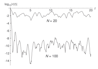
Figure 1: Plot of $\log_{10}|r(t)|$, with the decoherence factor $r(t)$ given by Eq. (14), for two different bath sizes $N=20$ and $100$. Fast decay of $r(t)$, corresponding to local decoherence, is observed, and the degree of decoherence is seen to increase with $N$. The squared coefficients $|\alpha_{i}|^{2}$ and the couplings $g_{i}$ were drawn from a uniform random distribution over the intervals $[0,1]$ and $[-\pi,\pi]$, respectively.

IV.3 Expectation values of global observables

An arbitrary global observable $\widehat{O}\equiv\widehat{O}_{\mathcal{SE}}$ can be written as a linear combination of the form $\widehat{O}=\sum_{\lambda\lambda^{\prime}}O_{\lambda\lambda^{\prime}}|{\phi_{\lambda}\rangle}{\langle\phi_{\lambda^{\prime}}}|$, where the $|{\phi_{\lambda}\rangle}$ are product eigenstates of the total Hamiltonian $\widehat{H}_{\mathcal{SE}}$, Eq. (7). Explicitly,

$$\widehat{O}=\sum_{j}\bigl{(}s^{(j)}_{00}|{0\rangle}{\langle 0}|+s^{(j)}_{01}|{0\rangle}{\langle 1}|+s^{(j)}_{10}|{1\rangle}{\langle 0}|+s^{(j)}_{11}|{1\rangle}{\langle 1}|\bigr{)}\\ \,\,\,\bigotimes_{i=1}^{N}\,\bigl{(}\epsilon^{(ij)}_{\uparrow\uparrow}|{\uparrow_{i}\rangle}{\langle\uparrow_{i}}|+\epsilon^{(ij)}_{\uparrow\downarrow}|{\uparrow_{i}\rangle}{\langle\downarrow_{i}}|+\epsilon^{(ij)}_{\downarrow\uparrow}|{\downarrow_{i}\rangle}{\langle\uparrow_{i}}|+\epsilon^{(ij)}_{\downarrow\downarrow}|{\downarrow_{i}\rangle}{\langle\downarrow_{i}}|\bigr{)}.$$ (18)

Since $\widehat{O}$ must be Hermitian, $s_{00}$, $s_{11}$, $\epsilon^{(i)}_{\uparrow\uparrow}$, and $\epsilon^{(i)}_{\downarrow\downarrow}$ are real numbers, and $s_{01}=\bigl{(}s_{10}\bigr{)}^{*}$, $\epsilon^{(i)}_{\downarrow\uparrow}=\bigl{(}\epsilon^{(i)}_{\uparrow\downarrow}\bigr{)}^{*}$. To keep the notation simple, we shall omit the sum over $j$ (and thus the index $j$) in the following.

The expectation value of $\widehat{O}$ in the state $|{\Psi(t)\rangle}$, Eq. (9), is

$$\langle\widehat{O}\rangle_{\Psi(t)} = \bigl{(}|a|^{2}s_{00}+|b|^{2}s_{11}\bigr{)}\prod_{i=1}^{N}\bigl{[}|\alpha_{i}|^{2}\epsilon^{(i)}_{\uparrow\uparrow}+\alpha_{i}^{*}\beta_{i}\epsilon^{(i)}_{\uparrow\downarrow}e^{-ig_{i}t}+\bigl{(}\alpha_{i}^{*}\beta_{i}\epsilon^{(i)}_{\uparrow\downarrow}\bigr{)}^{*}e^{ig_{i}t}+|\beta_{i}|^{2}\epsilon^{(i)}_{\downarrow\downarrow}\bigr{]}$$ (19)

$$+\,2\,\text{Re}\biggl{(}ab^{*}s_{10}\prod_{i=1}^{N}\bigl{[}|\alpha_{i}|^{2}\epsilon^{(i)}_{\uparrow\uparrow}e^{ig_{i}t}+\alpha^{*}_{i}\beta_{i}\epsilon^{(i)}_{\uparrow\downarrow}+\bigl{(}\alpha_{i}^{*}\beta_{i}\epsilon^{(i)}_{\uparrow\downarrow}\bigr{)}^{*}+|\beta_{i}|^{2}\epsilon^{(i)}_{\downarrow\downarrow}e^{-ig_{i}t}\bigr{]}\biggr{)}$$

$$\equiv \bigl{(}|a|^{2}s_{00}+|b|^{2}s_{11}\bigr{)}\Gamma_{0}(t)+2\,\text{Re}\bigl{[}ab^{*}s_{10}\Gamma_{1}(t)\bigr{]}.$$

The special case of the expectation value of local observables, as considered in the preceding Sec. IV.2, can easily be recovered by remembering that tracing out the degrees of freedom of $\mathcal{E}$ is equivalent to choosing all coefficients $\epsilon^{(i)}_{\uparrow\uparrow}=\epsilon^{(i)}_{\downarrow\downarrow}=1$ and $\epsilon^{(i)}_{\uparrow\downarrow}=\bigl{(}\epsilon^{(i)}_{\downarrow\uparrow}\bigr{)}^{*}=0$, which yields $\Gamma_{0}(t)=1$ and $\Gamma_{1}(t)=r(t)$ [see Eq. (14)], in agreement with Eq. (16).

Suppression of terms in $\langle\widehat{O}\rangle_{\Psi(t)}$ that are not diagonal in the energy eigenbasis would be represented by the vanishing of all time-dependent terms in the above expression, i.e.,

$$\langle\widehat{O}\rangle_{d} = \bigl{(}|a|^{2}s_{00}+|b|^{2}s_{11}\bigr{)}\prod_{i=1}^{N}\big{(}|\alpha_{i}|^{2}\epsilon^{(i)}_{\uparrow\uparrow}+|\beta_{i}|^{2}\epsilon^{(i)}_{\downarrow\downarrow}\big{)}$$ (20)

$$\,+2\,\text{Re}\biggl{(}ab^{*}s_{10}\prod_{i=1}^{N}2\,\text{Re}\bigl{(}\alpha^{*}_{i}\beta_{i}\epsilon^{(i)}_{\uparrow\downarrow}\bigr{)}\biggr{)}$$

$$\equiv \bigl{(}|a|^{2}s_{00}+|b|^{2}s_{11}\bigr{)}\Gamma^{d}_{0}+2\,\text{Re}\bigl{(}ab^{*}s_{10}\Gamma^{d}_{1}\bigr{)},$$

because we can easily show that $\langle\widehat{O}\rangle_{d}=\text{Tr}(\rho_{d}\widehat{O})$, where $\rho_{d}$, Eq. (12), is the part of the density matrix that is diagonal in the eigenstates of the total Hamiltonian. We also see that $\langle\widehat{O}\rangle_{d}=\text{Tr}(\rho\widehat{O}_{d})$, where

$$\begin{split}\widehat{O}_{d}&=\bigl{(}s_{00}|{0\rangle}{\langle 0}|+s_{11}|{1\rangle}{\langle 1}|\bigr{)}\bigotimes_{i=1}^{N}\,\bigl{(}\epsilon^{(i)}_{\uparrow\uparrow}|{\uparrow_{i}\rangle}{\langle\uparrow_{i}}|+\epsilon^{(i)}_{\downarrow\downarrow}|{\downarrow_{i}\rangle}{\langle\downarrow_{i}}|\bigr{)}\\ &+\bigl{(}s_{01}|{0\rangle}{\langle 1}|+s_{10}|{1\rangle}{\langle 0}|\bigr{)}\bigotimes_{i=1}^{N}\,\bigl{(}\epsilon^{(i)}_{\uparrow\downarrow}|{\uparrow_{i}\rangle}{\langle\downarrow_{i}}|+\epsilon^{(i)}_{\downarrow\uparrow}|{\downarrow_{i}\rangle}{\langle\uparrow_{i}}|\bigr{)}.\end{split}$$ (21)

is the part of $\widehat{O}$ diagonal in energy. Thus, as expected, diagonality of $\langle\widehat{O}\rangle_{\Psi(t)}$ in energy can also be characterized by the presence of only those product expansion coefficients that are contained in $\widehat{O}_{d}$.

The form of the two product terms $\Gamma_{0}(t)$ and $\Gamma_{1}(t)$ is similar: They only differ in the order of the pairing of the product expansion coefficients with the exponential factors. Also, since the coefficients $s_{jj^{\prime}}$ are independent, diagonalization in energy will in general require that individually $\Gamma_{j}(t)\rightarrow\Gamma_{0}^{d}$ and $\Gamma_{1}(t)\rightarrow\Gamma_{1}^{d}$ for large $t$. We can therefore restrict our following analysis to $\Gamma_{0}(t)$ alone. (We shall also omit the subscript “0” in the following.)

First of all, let us rewrite $\Gamma(t)$ as a sum of $4^{N}$ terms,

$$\Gamma(t)=\sum_{\lambda}c_{\lambda}e^{iE_{\lambda}t}.$$ (22)

where the $c_{\lambda}$ represent products of expansion coefficients,

$$c_{\lambda} = \biggl{(}\prod_{i\in I_{1}(\lambda)}|\alpha_{i}|^{2}\epsilon^{(i)}_{\uparrow\uparrow}\biggr{)}\biggl{(}\prod_{i\in I_{2}(\lambda)}|\beta_{i}|^{2}\epsilon^{(i)}_{\downarrow\downarrow}\biggr{)}$$ (23)

$$\times \biggl{(}\prod_{i\in I_{3}(\lambda)}\alpha_{i}^{*}\beta_{i}\epsilon^{(i)}_{\uparrow\downarrow}\biggr{)}\biggl{(}\prod_{i\in I_{4}(\lambda)}\bigl{(}\alpha^{*}_{i}\beta_{i}\epsilon^{(i)}_{\uparrow\downarrow}\bigr{)}^{*}\biggr{)}.$$

Here the sets $I_{k}(\lambda)$ specify over which indices $i$ each product runs, namely, they are subsets of the set $I=\{1,\ldots,N\}$ of all integers between 1 and $N$ such that $\cup_{k}I_{k}(\lambda)=I$ and $\cap_{k}I_{k}(\lambda)=\emptyset$. The total energy $E_{\lambda}$ associated with each term in the sum, Eq. (22), is

$$E_{\lambda}=\sum_{i\in I_{4}(\lambda)}g_{i}-\sum_{i\in I_{3}(\lambda)}g_{i}.$$ (24)

We choose the index $\lambda$ such that $E_{\lambda-1}\leq E_{\lambda}\leq E_{\lambda+1}$ for all $\lambda$. Clearly, $E_{\lambda}=0$ whenever $I_{3}(\lambda)=I_{4}(\lambda)=\emptyset$ [i.e., if $I_{1}(\lambda)\cup I_{2}(\lambda)=I$], canceling out the time dependence of the associated product term in the expression for $\Gamma(t)$. Thus, we can split $\Gamma(t)$ into a time-independent and a time-dependent part,

$$\Gamma(t) = \sum_{\lambda}c_{\lambda}+\sum_{\lambda}c_{\lambda}e^{iE_{\lambda}t}\equiv\Gamma^{d}+\Lambda(t),$$ (25)

where now the first sum runs over all $\lambda$ for which $I_{1}(\lambda)\cup I_{2}(\lambda)=I$, while the second sum runs over all $\lambda$ for which $I_{3}(\lambda)\cup I_{4}(\lambda)\not=\emptyset$.

Diagonality in energy would require $\Lambda(t)\rightarrow 0$ as $t\rightarrow\infty$. Written this way, we see that $\Lambda(t)$ is formally similiar to the function $r(t)$ derived for local observables, Eq. (17). This might not come as a surprise, since also the expression for $r(t)$ can be derived from the calculation of an expectation value of an observable, namely, that of the local observable $\widehat{O}_{r}=(|{0\rangle}{\langle 1}|+|{1\rangle}{\langle 0}|)\bigotimes_{i=1}^{N}\,\widehat{I}_{k}$ that measures the degree of local interference between the $\mathcal{S}$ states $|{0\rangle}$ and $|{1\rangle}$. However, in the case of $r(t)$, $c_{\lambda}=|{\langle\phi_{\lambda}}|{\Psi_{0}\rangle}|^{2}$ is a product of $N$ real and non-negative coefficients $|\alpha_{i}|^{2}$ and $|\beta_{i}|^{2}=1-|\alpha_{i}|^{2}$, while the $c_{\lambda}$ of Eq. (23) contain cross terms of the form $\alpha_{i}\beta_{i}^{*}$ and $\alpha_{i}^{*}\beta_{i}$, arbitrary real coefficients $\epsilon^{(i)}_{\uparrow\uparrow}$ and $\epsilon^{(i)}_{\downarrow\downarrow}$, and arbitrary complex coefficients $\epsilon^{(i)}_{\uparrow\downarrow}$.

We expect this difference to have strong influence on the time evolution of $\Lambda(t)$ vs that of $r(t)$. The destructive interference needed to obtain suppression of the off-diagonal part of the expectation value relies on the idea that, when a function $f(z)$ is multiplied by a phase factor $e^{izt}$ whose variation with $z$ is much faster than that of $f(z)$, neighboring values $f(z)$ and $f(z+\delta z)$ will have similiar magnitude and phases, but will be weighted with two strongly different phase factors, which leads to an averaging-out effect in the sum $\sum_{z}f(z)e^{izt}$.

In our case, writing

$$\Lambda(t)=\sum_{\lambda}r_{\lambda}e^{i\varphi_{\lambda}}e^{iE_{\lambda}t},$$ (26)

with $r_{\lambda}=|c_{\lambda}|$, the phases $\varphi_{\lambda}$ will in general vary very rapidly with $\lambda$ and, thus, with $E_{\lambda}$. This is a consequence of the fact that the $c_{\lambda}=r_{\lambda}e^{i\varphi_{\lambda}}$ are composed of products of coefficients, such that changing a single term in the product will in general result in a drastic change in the overall phase associated with the $c_{\lambda}$. (The variation in magnitude among the $c_{\lambda}$ can be expected to be comparably insignificant for larger $N$.) Such discontinuous phase fluctuations are absent in the formally similiar function $r(t)$, Eq. (14), since there only the absolute value of the coefficients $\alpha_{i}$ and $\beta_{i}$ enters. Note that the impact of the phase fluctuations cannot be diminished by going to larger $t$, since the $2\pi$ periodicity of phases implies that the effect of a phase difference between terms $\lambda$ and $\lambda+1$ induced by $e^{i(E_{\lambda+1}-E_{\lambda})t}$ will in average be similiar to that induced by $e^{i(\varphi_{\lambda+1}-\varphi_{\lambda})}$ for all (larger) values of $t$.

We anticipate the described phase-variation effect to counteract the averaging-out influence of the multiplying phase factor $e^{-iEt}$, and to thus make it more difficult, if not entirely impossible, for $\Lambda(t)$, Eq. (25), to converge to zero. On the other hand, if the average difference between the phases associated with the individual coefficients is decreased, we would expect that the rate and degree of decay of $\Lambda(t)$ will be improved.

IV.4 Numerical results for the expectation value of random global observables

To check this prediction and to generally gain more insight into the behavior of $\langle\widehat{O}\rangle_{\Psi(t)}$, Eq. (19), we studied numerically the time evolution of $\Lambda(t)$, Eq. (26), normalized by its initial value at $t=0$, for sets of random observables $\widehat{O}$. Diagonalization of $\langle\widehat{O}\rangle_{\Psi(t)}$ in energy would then be represented by a decay of $\Lambda(t)$ from its initial value of one.

Figure 2 shows three typical examples for the time evolution of $\log_{10}\Lambda(t)$ for a fixed bath size of $N=100$. All couplings $g_{i}$ were taken to be random real numbers between $-\pi$ and $\pi$. To investigate the influence of phase fluctuations of the $c_{\lambda}$, Eq. (23), we considered three different cases for selecting the coefficients $\alpha_{i}$, $\beta_{i}$, $\epsilon^{(i)}_{\uparrow\uparrow}$, $\epsilon^{(i)}_{\downarrow\downarrow}$, and $\epsilon^{(i)}_{\uparrow\downarrow}$, i.e., for choosing the initial state of the environment and the observable. In the completely random case (A), the coefficients $\alpha_{i}$, $\beta_{i}$, and $\epsilon^{(i)}_{\uparrow\downarrow}$ were taken to be random complex numbers, with magnitudes and phases drawn from a uniform distribution over the intervals $[0,1]$ and $[0,2\pi]$, respectively (and such that $|\beta_{i}|^{2}=1-|\alpha_{i}|^{2}$). Similiarly, the coefficients $\epsilon^{(i)}_{\uparrow\uparrow}$ and $\epsilon^{(i)}_{\downarrow\downarrow}$ were random real numbers drawn from a uniform distribution over the interval $[-1,1]$. In the second case (B), the initial state of the environment was prepared such that the phases of the $\alpha_{i}$ and $\beta_{i}$ were restricted to the interval $[0,\pi/2]$. Also, only observables with non-negative values of $\epsilon^{(i)}_{\uparrow\uparrow}$ and $\epsilon^{(i)}_{\downarrow\downarrow}$ were considered, such that sign reversals of $c_{\lambda}$ due to a change of product terms containing these coefficients were prevented. Finally, in the third case (C), only the absolute values of the $\alpha_{i}$, $\beta_{i}$, $\epsilon^{(i)}_{\uparrow\uparrow}$, $\epsilon^{(i)}_{\downarrow\downarrow}$, and $\epsilon^{(i)}_{\uparrow\downarrow}$ were used, which implies that the $c_{\lambda}$ fluctuated only in magnitude.

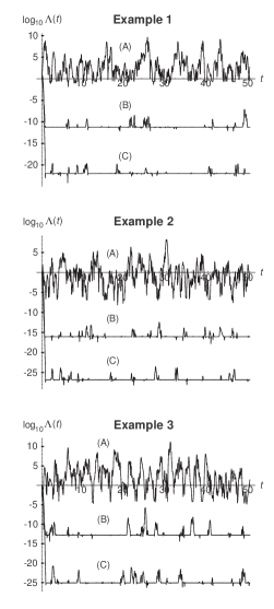
Figure 2: Time evolution of $\log_{10}\Lambda(t)$ [see Eq. (26)] for $N=100$ bath spins and three different random observables and initial states of the environment. The function $\Lambda(t)$ quantifies the time dependence of the terms in the expectation value $\langle\widehat{O}\rangle_{\Psi(t)}$ [Eq. (19)] that are not diagonal in energy. Suppression of these terms is represented by a decay of $\Lambda(t)$ from its initial value of one [i.e., $\log_{10}\Lambda(t)\longrightarrow-\infty$]. It is observed that in the general case (A) of completely random observables and initial states of the environment, collective decay of off-diagonal terms does, in general, not occur. However, if the phases of the coefficients describing the observable and the environment are moderately restricted (B) or all set equal to zero (C), decay of increasing strength is found.

We observed a drastic influence of the range of phases and signs associated with the individual coefficients $\alpha_{i}$, $\beta_{i}$, $\epsilon^{(i)}_{\uparrow\downarrow}$, $\epsilon^{(i)}_{\uparrow\uparrow}$, and $\epsilon^{(i)}_{\downarrow\downarrow}$, on the evolution of $\Lambda(t)$. In the special case (C) of all coefficients being real non-negative numbers, $\Lambda(t)$ exhibited a consistently strong and fast decay behavior, similiar to the decay of the function $r(t)$, Eq. (14), describing suppression of off-diagonal terms for local observables (see Fig. 1). In the intermediate case (B), with restricted phases and signs, the degree of decay of $\Lambda(t)$ was decreased, while the decay rate stayed roughly the same. In the general random case (A), in which no restriction on the spread of phases and on the signs of the coefficients was imposed, the time evolution of $\Lambda(t)$ was observed to be sensitive to the particular set of random numbers used for the coefficients $\alpha_{i}$, $\beta_{i}$, $\epsilon^{(i)}_{\uparrow\downarrow}$, $\epsilon^{(i)}_{\uparrow\uparrow}$, and $\epsilon^{(i)}_{\downarrow\downarrow}$ in each run. For some of the sets, $\Lambda(t)$ was seen to lack any decay behavior at all. In other cases, the baseline of oscillation was located below zero, indicating a very weak damping effect, albeit with the peaks of the large-amplitude oscillation frequently reaching values greater than zero.

These results show that, for the bath size studied here, a consistent occurence of a decay of $\Lambda(t)$ hinges on the phase restrictions imposed on the coefficients describing the observable and the initial state of the environment. If these restrictions are given up, the time evolution of $\Lambda(t)$ and any occurence of a (comparably weak) decay will exhibit strong dependence on the particular set of values chosen for the coefficients.

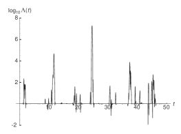
Figure 3: Time evolution of $\log_{10}\Lambda(t)$ for $N=100$ bath spins [see Eq. (26)] when no restrictions on the initial state of the environment are imposed. Such restrictions are physically unrealistic and require a preparing measurement on the unrestricted environment, which would in turn be in conflict with the desired generality of the derivation of decay effects. No collective decay of off-diagonal terms is observed, regardless of any restrictions imposed on the observable.

However, it is important to realize that the assumption of a restricted initial state of $\mathcal{E}$ is not only unrealistic, since the environment is typically uncontrollable, but it will also lead to a circular argument when aiming at a derivation of a universal decay effect. This is so because any restriction would require an appropriate preparation of the initial state through a measurement on the entire $\mathcal{E}$, which implies that suppression of off-diagonal terms would then in general be absent for the observable corresponding to this measurement, if the restriction of the initial state of $\mathcal{E}$ is relevant to the occurence of the suppression. Consequently, the $\alpha_{i}$ and $\beta_{i}$ must be allowed to possess arbitrary phases. Then, since the $\epsilon^{(i)}_{\uparrow\uparrow}$, $\epsilon^{(i)}_{\downarrow\downarrow}$, and $\epsilon^{(i)}_{\uparrow\downarrow}$ are always paired with the $\alpha_{i}$ and $\beta_{i}$ in the expression for the $c_{\lambda}$ that make up $\Lambda(t)$ [see Eq. (23)], we anticipate that giving up phase restrictions on the $\alpha_{i}$ and $\beta_{i}$ will render the restrictions imposed on the $\widehat{O}$-coefficients less effective, if not entirely irrelevant, in bringing about a decay of $\Lambda(t)$.

To study this prediction, in Fig. 3 we show a representative plot of $\Lambda(t)$ using only the absolute values of the $\widehat{O}$ coefficients $\epsilon^{(i)}_{\uparrow\uparrow}$, $\epsilon^{(i)}_{\downarrow\downarrow}$, and $\epsilon^{(i)}_{\uparrow\downarrow}$, but with the $\mathcal{E}$ coefficients $\alpha_{i}$ and $\beta_{i}$ possessing random phases between 0 and $2\pi$. We found that decay is either entirely absent or strongly diminished in strength, despite the fact that the strongest possible restriction on the phases and signs of the $\widehat{O}$ coefficients is imposed. Similiar to the case of completely random coefficients, the behavior of $\Lambda(t)$ was observed to depend crucially on the particular set of random numbers chosen for the coefficients. These results lead us to conclude that a universal decay of off-diagonal terms does not occur for the studied bath size and time scale.

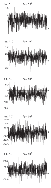
Figure 4: Example for the time evolution of $\log_{10}\Lambda(t)$ [see Eq. (26)] using a random observable and random initial bath state, for bath sizes between $N=10^{2}$ and $10^{6}$ and a long time scale $t=0$–$10^{6}$. No connection between the size of the spin bath and the occurrence and the degree of damping is observed. Therefore, no consistent collective decay of interference terms occurs. The increased time scale is seen to be irrelevant.

To be sure, SID is based on the assumption of a quasicontinuous energy spectrum and very long time scales, corresponding to “sufficiently large” $N$ and $t$ (the existing derivations of SID Castagnino and Lombardi (2004); Castagnino and Gadella (2003); Castagnino and Lombardi (2003); Castagnino and Ordóñez (2001); Castagnino et al. (2001); Castagnino and Laura (2000a, b, c); Laura et al. (1999); Castagnino (1999); Laura and Castagnino (1998a, b); Castagnino and Laura (1997) even assume the strict limits $N\rightarrow\infty$ and $t\rightarrow\infty$, in order to allow for a direct application of the Riemann-Lebesgue theorem), while so far we have only considered relatively modest values for these parameters. However, since we know from Fig. 1 that for expectation values of local observables, strong and fast decay of off-diagonal terms is obtained for the value of $N$ and over the time scale used in the plots shown in Fig. 2, it is clear that, if a general global disappearance of interference terms is to occur in our model, it will require a much larger number of environmental qubits and/or longer time scales than typically considered for local observables.

Accordingly, in Fig. 4 we show a typical example for the time evolution of $\Lambda(t)$ over the time scale $t=0$–$10^{6}$ for the case of a completely random observable and initial state of $\mathcal{E}$, using comparably large bath sizes $N$ between $N=10^{2}$ and $10^{6}$. We observed that even for these values of $N$, no consistent occurrence of a decay became apparent. In particular, no generally valid direct correlation between the value of $N$ and the time evolution of $\Lambda(t)$ was visible. Instead, it was again the particular set of random numbers included in the computation of $\Lambda(t)$ for a given value of $N$ (but not to the size $N$ of the set itself) that determined whether the baseline of oscillation of $\Lambda(t)$ was located above or below the zero line. In agreement with analytical predictions in the preceding section, we also found that the choice of a longer timescale is irrelevant, since neither the baseline nor the amplitude of oscillation changed significantly over the investigated time interval after a comparably short initial period. Furthermore, we observed that even if $\Lambda(t)$ “decayed” for a particular set of random numbers, the function sustained a large-amplitude oscillation whose peaks often attained values much larger than the initial value of $\Lambda(t)$.

Our results show that, in general, for the bath sizes and time scales studied, destructive interference of off-diagonal terms in the expectation value expressed in the energy eigenbasis [as quantified by $\Lambda(t)$, see Eq. (26)] does not occur in our model. Instead, the time evolution of $\Lambda(t)$ is simply determined by the particular random numbers used to describe the observable and the initial state of the environment. Therefore, no general suppression of interference terms can be inferred.

V Discussion

The process described by SID appears to be neither formally nor conceptually nor physically related to the decoherence mechanism in the standard sense of environmental decoherence. EID accounts for the absence of interference from the perspective of the local (open) system by describing interactions with an environment in quantum-mechanical terms of wave-function entanglement. In contrast, SID describes dynamically induced destructive interference between time-dependent terms in the expression for expectation values. SID does not, however, explain the physical origin of the measurement outcomes and their probability-weighted ensembles needed to define the expectation values. Even if this purely phenomenological basis of SID is accepted, the described process has no bearing on a loss of coherence in individual measurements, since it is only a consequence of averaging over a large number of measurement results. This is in fundamental contrast to EID, where each measurementlike interaction leads to a dislocalization of interference and thus, locally, to a disappearance of interference.

The main result of our study of the spin bath model is the finding that the destructive interference predicted by SID will in general fail to occur in our model even for bath sizes and over time scales much larger than typically considered in treatments of the same model in environmental decoherence. The source of this failure lies in the random relative phases associated with the individual initial bath spin states and the expansion coefficients of the observable. The resulting discontinuous phase fluctuations in the coefficient function $c_{\lambda}$, as defined in Eq. (23), counteract the supposed averaging-out effect of the dynamical phase factors $e^{iEt}$ in a way that is, due to the $2\pi$ periodicity of the phase, effectively independent of the value of $t$.

Even when the bath size is increased, the function $c_{\lambda}$ remains a set of discrete values with discontinuously varying phases. This can be explained by noting that, while the total energy is a sum of the energies of each subsystem, such that enlarging the number of contributing subsystems will in general lead to an improved quasicontinuity of the energy spectrum, the $2\pi$ periodicity of the phases implies that the degree of phase discontinuity of the $c_{\lambda}$ will not be diminished by increasing the number of subsystems. It is therefore unlikely that a consistent decay behavior could become apparent for spin baths much larger than those considered here.

This indicates that it is not the degree of continuity of the energy spectrum that represents the determining factor for obtaining destructive interference. Rather, it is the discrete nature of the model itself that seems to lead to difficulties. Only if restrictions are imposed on both the measured observable and the initial state of the environment, a consistent and general suppression of off-diagonal terms can occur. But, as we have argued, the corresponding preparation of the initial state of the environment is physically unrealistic and renders the derivation of a universal decay effect circular.

We conjecture that the diagonalization of the expectation value, as described by SID, is likely to fail also in other systems composed of discrete individual subentities. For, in such models, the relevant function will typically be represented by a large product of discrete expansion coefficients, similiar to the $c_{\lambda}$ of our model, whose discontinuous phase fluctuations will again be likely to counteract the averaging-out influence of the dynamical phases. It is therefore clear that the seemingly innocuous mathematical requirement of regularity and integrability of the coefficient functions (see Sec. II) is far from “valid in all relevant cases” where the condition of a sufficiently continuous energy spectrum holds. The suggestion to approximate such discrete functions by a continuous function through interpolation Castagnino and Lombardi (2004) does not appear to be viable, since the interpolated function would describe a physically different situation.

On a general note, it is also important to realize that dynamical phases are correlated. Thus one could always construct an observable for which the initial phases of the coefficients seem completely random, but are in fact chosen such that recurrence of coherence will show up within a finite time interval, thus disproving the claimed universality of SID without any further argument.

VI Summary and conclusions

We have investigated the two main claims of the “self-induced decoherence” approach, namely, (1) that expectation values of observables pertaining to a closed system become diagonal in the eigenbasis of the Hamiltonian, provided the system is endowed with a continuous energy spectrum; and (2) that this process represents a new way of describing quantum decoherence, and that it leads to results equivalent to the standard approach of environment-induced decoherence.

We have evaluated the first claim in the context of a simple spin bath model of finite size by studying, analytically and numerically, the time evolution of expectation values of random global observables. We have found that, in general, collective decay of terms off-diagonal in the energy eigenbasis does not occur over the large range of bath sizes and time scales considered. This result is not due to an insufficient quasicontinuity of the energy spectrum, but is rather rooted in the randomness of the phases associated with the observable and the initial state of the environment. Even in the limit of large bath sizes, the discrete functions for which destructive interference is to be derived do not approach their sufficiently smoothly varying interpolated approximations required for the dynamical phase averaging to have an effect.

These results represent an example for a simple model system that, although endowed with a quasicontinuous energy spectrum, fails to exhibit the decay of off-diagonal terms that would be expected from an extrapolation of SID to discrete models in the limit of comparably large sizes of the system. Such an extrapolation should be possible if the approach is to have general physical relevance. We have also anticipated that the decay effect described by SID will likely be absent also in other similiar models that are composed of discrete subsystems.

With respect to the second claim of the SID program, we have questioned the suggestion that SID represents a “new viewpoint” Castagnino and Lombardi (2004) on the theory of environment-induced decoherence, since the two approaches are based on conceptually, formally, and physically unrelated mechanisms. In particular, we have pointed out the following key differences and objections.

(i) SID does not describe the suppression of interference for individual measurements, since interference terms in the expectation value are not damped individually.

(ii) SID simply presupposes the existence of an ensemble of measurement outcomes, without giving an account of its origin in terms of a physical description of measurement.

(iii) The assumption of closed systems is unrealistic, especially for systems containing the many degrees of freedom needed to obtain the required quasicontinuous energy spectrum.

(iv) The physical feasibility and relevance of measurements pertaining to the total system-environment combination is doubtful.

(v) Energy as the universal preferred basis of the global closed system can usually not account for the different observed preferred bases for the local system of interest.

Our study leads us to two main conclusions. First, it points to the need for more precise, physically motivated criteria for the occurrence of the destructive interference effect described by SID. Most importantly, however, the physical interpretation and relevance of this effect need to be explained. We suspect that the SID approach may have mistakenly interpreted and labeled an unrelated process as “decoherence.”