Simulation of Quantum Computation: A deterministic event-based approach

Abstract

We demonstrate that locally connected networks of machines that have primitive learning capabilities can be used to perform a deterministic, event-based simulation of quantum computation. We present simulation results for basic quantum operations such as the Hadamard and the controlled-NOT gate, and for seven-qubit quantum networks that implement Shor’s numbering factoring algorithm.

I Introduction

Recent advances in nanotechnology are paving the way to attain control over individual microscopic objects CHIO04 ; RUGA04 ; ELZE04 ; XIAO04 ; FUJI03 . The ability to prepare, manipulate, couple and measure single quantum systems is essential for quantum computation NIEL00 . Candidate systems to implement a quantum computer are ions or atoms in electromagnetic or optical traps, photons in cavities, nuclear spins on molecules, quantum dots and superconductors. These technological developments facilitate the study of single quantum systems at the level of individual events. Such experiments address the most fundamental aspects of quantum theory. Indeed, quantum theory gives us only a recipe to compute the frequencies for observing events. It does not describe individual events, such as the arrival of a single electron at a particular position on the detection screen FEYN65 ; HOME97 ; TONO98 ; BALL03 . Reconciling the mathematical formalism (that does not describe single events) with the experimental fact that each observation yields a definite outcome is often referred to as the quantum measurement paradox. This is the fundamental problem in the foundation of quantum theory FEYN65 ; HOME97 ; PENR90 .

In view of this, it is not a surprise that some of the most fundamental experiments in quantum physics have not been simulated in the event-by-event manner in which the experimental observations are actually recorded PerfectExperiments . One of the examples are the two-slit experiments in which the individual electron counts build up the interference pattern TONO98 . Other examples are the single-photon beam splitter and Mach-Zehnder interferometer experiments GRAN86 . Within the standard formalism of quantum theory, no algorithm has been found to perform an event-based simulation of definite individual outcomes in quantum experiments HOME97 .

In this paper, we take the point of view that a physical theory such as quantum theory, is a specification of an algorithm to compute numbers that can be compared to experimental data KAMP88 . Thinking in terms of algorithms opens new possibilities to simulate phenomena for which a proper physical theory is not (yet) available. As discussed before, quantum theory is unable to describe individual events in an experiment but it provides an algorithm to compute the final, collective outcome. We have already demonstrated that it is possible to construct deterministic processes that generate events at a rate that agrees with the quantum mechanical probability distribution, without using quantum theory KOEN04 . In this paper we apply these concepts to quantum computation. We present results of event-based simulations of single-qubit quantum interference (Mach-Zehnder interferometer), a two-qubit quantum circuit (controlled-NOT gate), and Shor’s algorithm SHOR99 to factorize $N=15$ on a seven qubit quantum computer.

The event-based simulation method that we describe in this paper is not a proposal for another interpretation of quantum mechanics. To avoid misunderstandings, we emphasize that our approach is not an extension of quantum theory. We simulate quantum systems without making use of the rules (algorithms) quantum theory provides us. However, the final, collective results of our event-by-event deterministic, causal learning processes are in perfect agreement with the probability distributions of quantum theory PENR90 . The event-based simulations build up the final outcome event-by-event, just like in real experiments. In physics terminology, the entire approach is particle-like and satisfies Einstein’s criteria of realism and causality HOME97 . In this sense, our approach can be viewed as a recipe to construct event-based systems, that is “classical” models, that behave as if they were “quantum mechanical”.

The paper is organized as follows. In Section II we briefly recall some basic elements of quantum computation. We describe the Hadamard, controlled-NOT (CNOT) and Toffoli gate, involving one, two or three qubits, repectively. We discuss the quantum network for the Mach-Zehnder interferometer and for Shor’s quantum algorithm to factorize $N=15$ on a seven-qubit quantum computer.

In Section III we introduce the deterministic learning machine (DLM) that is at the core of the event-based simulation approach. We present a mathematical analysis that proves that these machines generate events at a rate that agrees with the corresponding quantum mechanical probabilities. One of the essential features of (networks of) DLMs is that they process one event at a time. After applying a deterministic decision process to the input event and sending out an output event, a new input event can be processed. Another essential feature of DLMs is that they do not store information about individual events. Networks of DLMs are capable of unsupervised learning KOEN04 but they have very little in common with neural networks HAYK99 . The sequence of events that is generated by a DLM is stricly deterministic. This is modified in the stochastic learning machine (SLM). The event-by-event learning processes in a SLM are still deterministic and causal but the output events are randomly distributed. This modification is necessary if we want to mimic the apparent random order in which quantum events are detected in experiments GRAN86 ; TONO98 .

In Section IV we first describe the construction of DLM networks and present results from the event-based simulation of the Hadamard gate and the Mach-Zehnder interferometer, the latter showing that DLM-based networks correctly reproduce quantum interference phenomena. Then we describe how to simulate a CNOT gate using DLM and SLM networks. Finally, we present the simulation results of Shor’s number factoring algorithm SHOR99 implemented on DLM and SLM networks. A summary and outlook is given in Section V.

II Quantum Computation

This section summarizes those aspects of quantum computation that are necessary to understand the examples of quantum algorithms that we use in Section IV to demonstrate that local, causal and deterministic processes can simulate quantum computers on an event-by-event basis.

II.1 Preliminaries

The state of an elementary storage unit of a quantum computer, the quantum bit or qubit, is described by a two-dimensional vector of Euclidean length one. Denoting two orthogonal basis vectors of the two-dimensional vector space by $|0\rangle$ and $|1\rangle$, the state $|\Phi\rangle$ of the qubit can be written as a linear superposition of the basis states $|0\rangle$ and $|1\rangle$:

$$|\Phi\rangle=a_{0}|0\rangle+a_{1}|1\rangle,$$ (1)

where $a_{0}$ and $a_{1}$ are complex numbers such that $|a_{0}|^{2}+|a_{1}|^{2}=1$. The appearance of complex numbers suggests that one qubit can contain an infinite amount of information. However, it is impossible to retrieve all this information SCHI68 ; BAYM74 ; BALL03 . The result of inquiring about the state of the qubit, that is the outcome of a measurement, is either 0 or 1. The frequency of obtaining 0 (1) can be estimated by repeated measurement of the same state of the qubits and is given by $|a_{0}|^{2}$ ($|a_{1}|^{2}$) SCHI68 ; BAYM74 ; BALL03 .

According to quantum theory QuantumTheory , the internal state of a quantum computer with $L$ qubits is described by a unit vector (state vector) in a $D=2^{L}$ dimensional space (of complex numbers) NIEL00 . Adopting the convention of quantum computation literature NIEL00 , the state of an $L$-qubit quantum computer is represented by

$$|\Phi\rangle = a({0\ldots 00})|0\ldots 00\rangle+a({0\ldots 01})|0\ldots 01\rangle+\ldots+a({1\ldots 10})|1\ldots 10\rangle+a({1\ldots 11})|1\ldots 11\rangle$$ (2)

$$= a_{0}|0\rangle+a_{1}|1\rangle+\ldots+a_{2^{L}-2}|2^{L}-2\rangle+a_{2^{L}-1}|2^{L}-1\rangle,$$

where in the last line of Eq. (2), the binary representation of the integers $0,\ldots,2^{L-1}$ was used to denote $|0\rangle\equiv|0\ldots 00\rangle,\ldots,|2^{L}-1\rangle\equiv|1\ldots 11\rangle$ and $a_{0}\equiv a({0\ldots 00}),\ldots,a_{2^{L}-1}\equiv a({1\ldots 11})$. As usual, we normalize the state vector, that is $\langle\Phi|\Phi\rangle=1$, by rescaling the complex-valued amplitudes $a_{i}$ according to

$$\sum_{i=0}^{2^{L}-1}|a_{i}|^{2}=1.$$ (3)

The internal state of the quantum computer evolves in time according to a sequence of unitary transformations NIEL00 . A quantum algorithm is a sequence of such unitary operations. Of course, not every sequence corresponds to a meaningful computation. Furthermore, if a quantum algorithm cannot exploit the fact that the intermediate state of the quantum computer is described by a linear superposition of basis vectors, it will not be faster than its classical counterpart. As the unitary transformation may change all amplitudes simultaneously, a quantum computer is a massively parallel machine NIEL00 , at least in theory.

It has been shown that an arbitrary unitary operation can be written as a sequence of single qubit operations and the controlled-NOT (CNOT) operation on two qubits DIVI95a ; NIEL00 . Therefore, single-qubit operations and the CNOT operation are sufficient to construct a universal quantum computer NIEL00 . The final state of the quantum computer can be calculated by performing the (unitary) matrix-vector multiplications that correspond to the application of this sequence (determined by the quantum algorithm) of single-qubit and CNOT operations. According to quantum theory, the squares of the absolute values of the elements of the state vector are the probabilities for observing the quantum computer in one of its $2^{L}$ states.

The unitary time evolution of the internal state of the quantum computer is interrupted at the point where we inquire about the value of the qubits, that is as soon as we perform a measurement on the qubits. If we perform the readout operation on a qubit, we get a definite answer, either 0 or 1, and the information encoded in the superposition is lost. The process of measurement cannot be described by a unitary transformation HOME97 ; BALL03 . Therefore, we do not consider it to be part of a quantum algorithm.

II.2 Single-qubit operations

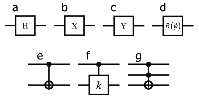
Figure 1: Graphical representation of some of the basic gates used in quantum computation; (a) Hadamard gate; (b) Rotation by $\pi/2$ about the $x$-axis; (c) Rotation by $\pi/2$ about the $y$-axis; (d) Single qubit phase shift by $\phi$; (e) CNOT gate; (f) Controlled phase shift by $\phi=\pi/k$; (g) Toffoli gate. The horizontal lines denote the qubits involved in the quantum operations. The dots and crosses denote the control and target qubits, respectively.

In general, a qubit can be represented by a spin-1/2 system. The state $|\Phi\rangle$ of a qubit (see Eq.(1)) can therefore also be written as a linear combination of the spin-up and spin-down states SCHI68 ; BAYM74 ; BALL03 :

$$|\Phi\rangle=a_{0}|\uparrow\rangle+a_{1}|\downarrow\rangle,$$ (4)

where NIEL00

$$|0\rangle=|\uparrow\rangle=\left(\begin{array}[]{c}1\\ 0\end{array}\right)\quad,\quad|1\rangle=|\downarrow\rangle=\left(\begin{array}[]{c}0\\ 1\end{array}\right).$$ (5)

The three components of the spin-1/2 operator ${\bf S}=(S^{x},S^{y},S^{z})$ are defined (in units such that ${\mathchar 22\relax\mskip-9.0muh}=1$) by SCHI68 ; BAYM74 ; BALL03

$$S^{x}=\frac{1}{2}\left(\begin{array}[]{cc}0&1\\ 1&0\end{array}\right),\quad S^{y}=\frac{1}{2}\left(\begin{array}[]{cc}\phantom{-}0&-i\\ \phantom{-}i&\phantom{-}0\end{array}\right),\quad S^{z}=\frac{1}{2}\left(\begin{array}[]{cc}\phantom{-}1&\phantom{-}0\\ \phantom{-}0&-1\end{array}\right),$$ (6)

and are chosen such that $|\uparrow\rangle$ and $|\downarrow\rangle$ are eigenstates of $S^{z}$ with eigenvalues +1/2 and -1/2, respectively.

The expectation values of the three components of the qubits are defined as

$$\langle Q^{\alpha}\rangle=1/2-\langle S^{\alpha}\rangle\quad,\quad\alpha=x,y,z,$$ (7)

where $\langle A\rangle=\langle\Phi|A|\Phi\rangle/\langle\Phi|\Phi\rangle$. A qubit is in the state $|0\rangle$ or $|1\rangle$ if $\langle Q^{z}\rangle=0$ or $\langle Q^{z}\rangle=1$, respectively.

A rotation of the state Eq.(4) about a vector ${\bf v}$ corresponds to the unitary matrix

$$e^{i{\bf v}\cdot{\bf S}}=\openone\cos\frac{v}{2}+\frac{2i{\bf v}\cdot{\bf S}}{v}\sin\frac{v}{2},$$ (8)

where $\openone$ denotes the unit matrix and $v=\sqrt{v_{x}^{2}+v_{y}^{2}+v_{z}^{2}}$ is the length of the vector ${\bf v}$.

For later reference, it is useful to list a few special cases of Eq.(8). The Hadamard operation $H$ and rotations $X$ and $Y$ of the state vector by $\pi/2$ about the $x$ and $y$-axis, respectively, are defined by NIEL00

$$H\equiv\frac{1}{\sqrt{2}}\left(\begin{array}[]{cc}\phantom{-}1&\phantom{-}1\\ \phantom{-}1&-1\end{array}\right),\quad X\equiv e^{i\pi S^{x}/2}=\frac{1}{\sqrt{2}}\left(\begin{array}[]{cc}1&i\\ i&1\end{array}\right),\quad Y\equiv e^{i\pi S^{y}/2}=\frac{1}{\sqrt{2}}\left(\begin{array}[]{cc}\phantom{-}1&\phantom{-}1\\ -1&\phantom{-}1\\ \end{array}\right).$$ (9)

We also introduce the symbol

$$R(\phi)=e^{i\phi/2}e^{-i\phi S^{z}}=\left(\begin{array}[]{cc}\phantom{-}1&\phantom{-}0\\ \phantom{-}0&\phantom{-}e^{i\phi}\end{array}\right),$$ (10)

to represent the single-qubit phase-shift operation by a phase $\phi$. The graphical symbols of $H$, $X$, $Y$, and $R(\phi)$ are shown in Fig. 1. The inverse of a unitary operation $U$ is denoted by $\overline{U}$.

Figure 2: Left: Diagram of the Mach-Zehnder interferometer, consisting of two beam splitters, two mirrors, and a device that changes the phase of the light wave by $\phi$. Right: Diagram of the equivalent quantum network.

The Mach-Zehnder interferometer is a simple but nontrivial example of a single-qubit system in which the information contained in the phase of the wave function is essential BORN64 ; GRAN86 ; RARI97 ; NIEL00 . The schematic layout of the apparatus is shown in Fig. 2. $N$ photons enter the first beam splitter through the input channels 0 or 1. The beam splitter distributes the photons over its two output channels (0 or 1): The number of photons in these channels is $N_{0}$ and $N_{1}$, respectively. If there are no photons in one of the input channels, the beam splitter equally divides the photons over its output channels, that is $N_{0}=N_{1}=N/2$. The photons then propagate and experience a phase shift of $\phi$ if they left the beam splitter via channel 1. The photons are collected at another beam splitter. Finally, detectors count the number of photons in the two output channels 0 and 1 of the second beam splitter. The number of photons in these channels is denoted by $N_{2}$ and $N_{3}$, respectively. We assume that no photons are lost in this process so that $N=N_{0}+N_{1}=N_{2}+N_{3}$.

The relation between input and output amplitudes of the Mach-Zehnder interferometer is given by BORN64 ; GRAN86 ; RARI97 ; NIEL00

$$\left(\begin{array}[]{c}b_{0}\\ b_{1}\end{array}\right)=XR(\phi)X\left(\begin{array}[]{c}a_{0}\\ a_{1}\end{array}\right)=\frac{1}{2}\left(\begin{array}[]{cc}1&i\\ i&1\end{array}\right)\left(\begin{array}[]{cc}1&0\\ 0&e^{i\phi}\end{array}\right)\left(\begin{array}[]{cc}1&i\\ i&1\end{array}\right)\left(\begin{array}[]{c}a_{0}\\ a_{1}\end{array}\right),$$ (23)

where ($a_{0},a_{1})$ and ($b_{0},b_{1})$ are the complex-valued amplitudes at the input and output, respectively. The $X$ operations represent the beam splitters while the phase shift $R(\phi)$ mimics the effect of changing the optical path length.

Let us consider the case where all the photons enter the interferometer through channel 0. Assuming that the photons originate from a coherent source, we have $(a_{0},a_{1})=(\cos\psi_{0}+i\sin\psi_{0},0)$. From Eq.(23) it follows that the probabilities for observing a photon at one of the output channels is given by

$$|b_{0}|^{2}=\sin^{2}\frac{\phi}{2},\quad|b_{1}|^{2}=\cos^{2}\frac{\phi}{2}.$$ (24)

II.3 Two qubits: CNOT operation and controlled phase shift

Computation requires some form of communication between the qubits. It has been shown that any form of communication between qubits can be reduced to a combination of single-qubit operations and the CNOT operation on two qubits DIVI95a ; NIEL00 . By defintion, the CNOT gate flips the target qubit if the control qubit is in the state $|1\rangle$ NIEL00 . If we take the first qubit (that is the least significant bit in the binary notation of an integer) as the control qubit, we have

$${\mathop{\hbox{CNOT}}}_{21}|\Phi\rangle = {\mathop{\hbox{CNOT}}}_{21}(a_{0}|00\rangle+a_{1}|01\rangle+a_{2}|10\rangle+a_{3}|11\rangle)$$ (25)

$$= a_{0}|00\rangle+a_{3}|01\rangle+a_{2}|10\rangle+a_{1}|11\rangle$$

$$= a_{0}|0\rangle+a_{3}|1\rangle+a_{2}|2\rangle+a_{1}|3\rangle$$

$$= a_{0}|0\rangle_{1}|0\rangle_{2}+a_{3}|1\rangle_{1}|0\rangle_{2}+a_{2}|0\rangle_{1}|1\rangle_{2}+a_{1}|1\rangle_{1}|1\rangle_{2}.$$

where $a_{0},\ldots,a_{3}$ are the probability amplitudes of the four different states and $|0\rangle_{i}$ and $|1\rangle_{i}$ represent the $|0\rangle$ and $|1\rangle$ state of the $i$-th qubit, respectively. The graphical symbol of the CNOT operation is shown in Fig. 1e. The dot (cross) denotes the control (target) qubit. A CNOT gate in which the control and target qubit are interchanged can be built from four Hadamard gates and one CNOT gate NIEL00 . The quantum circuit for this “reversed” CNOT gate is shown in Fig. 3.

The CNOT operation is a special case of the controlled phase shift operation $R_{ji}(\phi)$. The controlled phase shift operation with control qubit 1 and target qubit 2 reads

$$R_{21}(\phi)|\Phi\rangle = R_{21}(\phi)(a_{0}|00\rangle+a_{1}|01\rangle+a_{2}|10\rangle+a_{3}|11\rangle),$$ (26)

$$= a_{0}|00\rangle+\frac{(1+e^{i\phi})a_{1}+(1-e^{i\phi})a_{3}}{2}|01\rangle+a_{2}|10\rangle+\frac{(1-e^{i\phi})a_{1}+(1+e^{i\phi})a_{3}}{2}|11\rangle.$$

Graphically, the controlled phase shift $R_{ji}(\phi=\pi/k)$ is represented by a vertical line connecting a dot (control bit) and a box denoting a single qubit phase shift by $\pi/k$ (see Fig. 1f).

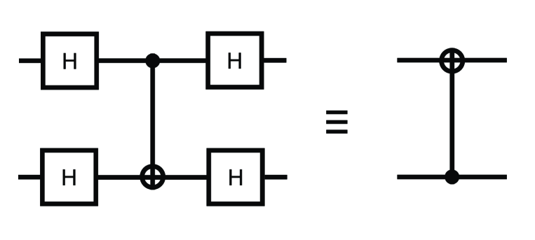
Figure 3: Quantum circuit representation of a CNOT gate where the second (bottom) qubit acts as control qubit and the first (top) qubit is the target qubit.

II.4 Three qubits: Toffoli gate

The Toffoli gate is a generalization of the CNOT gate in the sense that it has two control qubits and one target qubit BARE95 ; NIEL00 . The target qubit flips if and only if the two control qubits are set. Symbolically the Toffoli gate is represented by a vertical line connecting two dots (control bits) and one cross (target bit), as shown in Fig. 1g.

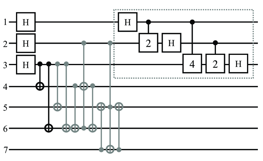
Figure 4: Quantum network for Shor’s quantum algorithm to find the factors of the number $N=15$ for the case $a=11$ (black colored CNOT gates only) and $a=7$ (gray colored CNOT and Toffoli gates only) SYPE01b . $H$ denotes the Walsh-Hadamard transform. The operations in the dashed box perform a 3-qubit Fourier transform NIEL00 . The operations “2” and “4” perform controlled phase shifts with angles $\pi/2$ and $\pi/4$, respectively. The other gates perform two-qubit (CNOT) or three-qubit (Toffoli) operations. The initial state of the seven qubits of the quantum computer is (0,0,0,0,0,0,1).

II.5 Seven qubits: Factoring $N=15$ using Shor’s algorithm

We now consider the problem of factoring integers. For the case $N=15$, an experimental realization of this quantum algorithm on a seven-qubit NMR quantum computer is described in Refs. SYPE01b, and SYPE01a, . The theory behind Shor’s algorithm has been discussed at great length elsewhere NIEL00 ; SHOR99 ; EKER96 . Therefore, we only recall the basic elements of Shor’s algorithm and focus on the implementation of the algorithm for the case $N=15$. The theory in this section closely follows Ref. SYPE01b, .

Shor’s algorithm is based on the fact that the factors $p$ and $q$ of an integer $N=pq$ can be deduced from the period $M$ of the function $f(j)=a^{j}{\mathop{\hbox{mod}}}N$ for $j=0,\ldots,2^{n}-1$ where $N\leq 2^{n}$. Here $a<N$ is a random number that has no common factors with $N$. Once $M$ has been determined, at least one factor of $N$ can be found by computing the greatest common divisor (g.c.d.) of $N$ and $a^{M/2}\pm 1$.

For $N=15$, the calculation of the modular exponentiation $a^{j}{\mathop{\hbox{mod}}}N$ is almost trivial. Using the binary representation of $j$ we can write $a^{j}{\mathop{\hbox{mod}}}N=a^{2^{n-1}j_{n-1}}\ldots a^{2j_{1}}a^{j_{0}}{\mathop{\hbox{mod}}}N=(a^{2^{n-1}j_{n-1}}{\mathop{\hbox{mod}}}N)\ldots(a^{2j_{1}}{\mathop{\hbox{mod}}}N)(a^{j_{0}}{\mathop{\hbox{mod}}}N){\mathop{\hbox{mod}}}N$, showing that we only need to implement $(a^{2^{k}j_{k}}{\mathop{\hbox{mod}}}N)$. For $N=15$ the allowed values for $a$ are $a=2,4,7,8,11,13,14$. If we pick $a=2,7,8,13$ then $a^{2^{k}}{\mathop{\hbox{mod}}}N=1$ for all $k>1$. For the remaining cases we have $a^{2^{k}}{\mathop{\hbox{mod}}}N=1$ for all $k>0$. Thus, for $N=15$ only two (not four) qubits are sufficient to obtain the period of $f(j)=a^{j}{\mathop{\hbox{mod}}}N$ SYPE01b . As a matter of fact, this analysis provides enough information to deduce the factors of $N=15$ using Shor’s procedure so that no further computation is necessary. Nontrivial quantum operations are required if we decide to use three (or more) qubits to determine the period of $f(j)=a^{j}{\mathop{\hbox{mod}}}N$ SYPE01b . Following Ref. SYPE01b, , we will consider a seven-qubit quantum computer with four qubits to hold $f(j)$ and three qubits to perform the Fourier transform to determine the period $M$.

The quantum circuit that implements Shor’s algorithm that factors $N=15$ using $a=7$ and $a=11$ is depicted in Fig. 4 SYPE01b . Qubits 1 to 3 and 4 to 7 are used as registers to represent $j$ and $f(j)=a^{j}{\mathop{\hbox{mod}}}N$, respectively. Here, qubits 3 and 7 are the least significant qubits of these two registers. The initial state of the qubits is $(0,0,0,0,0,0,1)$, that is, all qubits are prepared in the state $|0\rangle$ except for qubit 7 which is prepared in the state $|1\rangle$.

The quantum networks to compute $a^{j}{\mathop{\hbox{mod}}}15$ for $j=0,\ldots,7$ and a fixed input $a$ are easy to construct. Examples for $a=7$ (six CNOT and two Toffoli gates) and $a=11$ (two CNOT gates) are included in Fig. 4 SYPE01b . For example, consider the case $a=11=|1011\rangle$. If $j$ is odd then $11^{j}{\mathop{\hbox{mod}}}15=11$ and the network should leave $|1011\rangle$ unchanged. Otherwise, $11^{j}{\mathop{\hbox{mod}}}15=1$ and hence it should return $|0001\rangle$. The network for this operation consists of two CNOT gates that have as control qubit, the same least-significant qubit (qubit 3 in Fig. 4) of the three qubits that are input to the Fourier transform. The sequence of CNOT and Toffoli gates that performs similar operations for the other cases can be found in the same manner. In the NMR implementation, additional simplications of the $a=7$ circuit where necessary to render the experiment feasible SYPE01b . There is no need to do this here, so we use the circuits as shown in Fig. 4. Elsewhere, we describe a quantum computer emulator (QCE) that simulates models of ideal and physically realizable quantum computers RAED00 ; MICH03 ; RAED05 . The software distribution of QCE QCEDOWNLOAD contains an implemention of the circuits shown in Fig. 4, demonstrating that these circuits work correctly.

For the quantum network of Fig. 4, we can determine the period $M$ of the function $f(j)=a^{j}{\mathop{\hbox{mod}}}N$ from the expectation values of the first three qubits. The state of the quantum computer before it starts performing the Fourier transform can be written as

$$\frac{1}{\sqrt{N}}\sum_{j=0}^{N-1}|j\rangle|f(j)\rangle = \frac{1}{\sqrt{N}}\left\{\sum_{j=0}^{M-1}|j\rangle|f(j)\rangle+\sum_{j=M}^{2M-1}|j\rangle|f(j)\rangle+\dots\right\}$$ (27)

$$= \frac{1}{\sqrt{N}}\sum_{j=0}^{M-1}\left(|j\rangle+|j+M\rangle+\ldots\right)|f(j)\rangle,$$

where, in the last step, we used the periodicity of $f(j)$. Using the Fourier representation of $|j\rangle$ we obtain

$$\frac{1}{\sqrt{N}}\sum_{j=0}^{N-1}|j\rangle|f(j)\rangle = \frac{1}{N}\sum_{k=0}^{N-1}\sum_{j=0}^{M-1}e^{2\pi ikj/N}\left(1+e^{2\pi ikM/N}+e^{4\pi ikM/N}+\ldots+e^{2\pi ikM(L-1)/N}\right)|k\rangle|f(j)\rangle$$ (28)

$$+ \frac{1}{N}\sum_{k=0}^{N-1}\sum_{j=0}^{L-1}e^{2\pi ikj/N}e^{2\pi ikML/N}|k\rangle|f(j)\rangle,$$

where $L=\lfloor N/M\rfloor$ denotes the largest integer $L$ such that $ML\leq N$. In simple terms, $L$ is the number of times the period $M$ fits into the interval $[0,N-1]$. The probability $p_{q}(M)$ to observe the quantum computer in the state $|q\rangle$ is given by the expectation value of the (projection) operator $Q=|q\rangle\langle q|$. With the restriction on $f(j)$ that $f(j)=f(j^{\prime})$ implies $j=j^{\prime}$, we find

$$\langle Q\rangle=p_{q}(M) = \frac{M}{N^{2}}\left(\frac{\sin(\pi qML/N)}{\sin(\pi qM/N)}\right)^{2}+\frac{N-ML}{N^{2}}\frac{\sin(\pi qM(2L+1)/N)}{\sin(\pi qM/N)}.$$ (29)

The results for $p_{q}(M)$ in the case $N=8$ (three qubits) are given in Table 1. From Table 1 it follows directly that the expectation values of the qubits are ($\langle Q_{1}^{z}\rangle=\langle Q_{2}^{z}\rangle=\langle Q_{3}^{z}\rangle=0$) if the period $M=1$, ($\langle Q_{1}^{z}\rangle=\langle Q_{2}^{z}\rangle=0$, $\langle Q_{3}^{z}\rangle=0.5$) if the period $M=2$, ($\langle Q_{1}^{z}\rangle=0.5$, $\langle Q_{2}^{z}\rangle=0.375$, $\langle Q_{3}^{z}\rangle=0.34375$) if the period $M=3$, and ($\langle Q_{1}^{z}\rangle=0$, $\langle Q_{2}^{z}\rangle=\langle Q_{3}^{z}\rangle=0.5$) if the period $M=4$.

Thus, in this simple case of $N=15$, the periodicity of $f(j)$ can be unambiguously determined from the expectation values of the individual qubits. For $a=7$ we find ($\langle Q_{1}^{z}\rangle=0$, $\langle Q_{2}^{z}\rangle=0.5$, $\langle Q_{3}^{z}\rangle=0.5$) and hence the period $M=4$, yielding the correct factors g.c.d.$(7^{2}\pm 1,15)=3,5$ of $N=15$. Similarly, for $a=11$ we find ($\langle Q_{1}^{z}\rangle=0$, $\langle Q_{2}^{z}\rangle=0$, $\langle Q_{3}^{z}\rangle=0.5$) corresponding to the period $M=2$ and the factors g.c.d.$(11\pm 1,15)=3,5$.

Table 1: Probability $p_{q}(M)$ to observe the state $|q\rangle$ after performing the quantum Fourier transform on the periodic function $f(j)=f(j+M)$ for $j=0,\dots,7$.

$q$	$p_{q}(M=1)$	$p_{q}(M=2)$	$p_{q}(M=3)$	$p_{q}(M=4)$
0	1	0.5	0.34375	0.25
1	0	0.0	0.01451	0.00
2	0	0.0	0.06250	0.25
3	0	0.0	0.23549	0.00
4	0	0.5	0.31250	0.25
5	0	0.0	0.23549	0.00
6	0	0.0	0.06250	0.25
7	0	0.0	0.01451	0.00

III Event-based simulation of quantum phenomena

The conventional approach for simulating quantum systems (and quantum computers in particular) is to solve the time-dependent Schrödinger equation of the corresponding system QMvideo . In practice, this amounts to multiplying the state vector by a sequence of (many) unitary matrices RAED00 ; MICH03 ; RAED05 . According to quantum theory, the squares of the amplitudes of the final state of the quantum computer yield the probabilities for observing the quantum computer in a particular basis state. Once these probabilities are known, it is trivial to construct a random process that generates events according to these probabilities.

The approach we propose in this paper is radically different. We construct processes that generate events of which the ratio of occurrence agrees with quantum theory. Thus, adopting this method, we don’t use concepts of quantum theory at all: we don’t use wave functions or the Schrödinger equation and do not run into the fundamental measurement paradox HOME97 . In our approach, quantum mechanical behavior is the result of a causal, deterministic (or stochastic), event-based process.

In quantum physics an event corresponds to the detection of a photon, electron, etc. In our simulation approach an event is very much the same thing: It is the arrival of a message at the input port of a processing unit. In this paper we only consider networks of processing units in which only one message is traveling through the network at any time. Thus, the network receives an event at one of its inputs, processes the event and delivers the processed message through one of its output channels. After delivering this message the network can accept a new input event.

The key feature of our approach is a processing unit that we call deterministic learning machine (DLM). A DLM is a machine with an internal state that is updated according to a very simple, deterministic algorithm. A DLM responds to the input event by choosing from all possible alternatives, the internal state that minimizes the error between the input and the internal state itself. This deterministic decision process determines which type of event will be generated as output by the DLM. Furthermore, the same process generates different events in such a way that the number of each type of event is proportional to the corresponding probabilities of the quantum mechanical device that we want to simulate. The message contains information about the decision the DLM took while updating its internal state and, depending on the application, also contains other data that the DLM can provide. By updating its internal state, the DLM “learns” about the input events it receives and by generating new events carrying messages, it tells its environment about what it has learned. This primitive learning capability is the essence of our approach.

III.1 Deterministic learning machines

An extensive discussion of the internal operation and dynamic behavior of a DLM can be found in Refs. KOEN04 ; HANS05 . Therefore, in this paper, we briefly recall the basic ideas. As an example, we take a DLM that we use to simulate the Hadamard operation (see Section II). We first consider a DLM that accepts as input two different types of events (0 or 1), each event carrying a message consisting of two real numbers. The DLM learns from the input event by updating its internal vector. The internal state of the DLM is represented by a unit vector of four real numbers ${\bf x}=(x_{0},x_{1},x_{2},x_{3})$. The first (last) two elements of ${\bf x}$ are used to learn about the message carried by 0 (1) events. As an input event is either of type 0 or 1, the DLM receives a message with two real numbers, not with four. Therefore, the DLM uses its internal vector to supply the two missing real numbers. Thus, for a 0 event carrying the message ${\bf y}_{0}=(y_{0},y_{1})$, the input vector is ${\bf v}=(y_{0},y_{1},x_{2},x_{3})$ and for a 1 event carrying the message ${\bf y}_{1}=(y_{2},y_{3})$, the input vector is ${\bf v}=(x_{0},x_{1},y_{2},y_{3})$. Consider now the second possibility in which the DLM receives input in the form of four real numbers ${\bf v}=(v_{0},v_{1},v_{2},v_{3})$. Then, it is clear that it can skip the step of supplying the missing information and use the input ${\bf v}$ directly.

The DLM updates its internal vector by selecting from the eight candidate update rules $\{j=0,1,2,3;s_{j}=\pm 1\}$

$$w_{i,j}=s_{j}\sqrt{1+\alpha^{2}(x_{j}^{2}-1)}\delta_{i,j}+\alpha x_{i}(1-\delta_{i,j})$$ (30)

the update rule that minimizes the cost

$$C=-{\bf w}_{j}^{T}{\bf v}^{\phantom{T}}.$$ (31)

Note that ${\bf x}^{T}{\bf x}^{\phantom{T}}=1$ implies ${\bf w}_{j}^{T}{\bf w}_{j}^{\phantom{T}}=1$ for each of the $8$ update rules. The parameter $0<\alpha<1$ controls the learning process. If $j^{\prime}$ and $s^{\prime}$ denote the values of $j$ and $s_{j}$ that minimizes the cost Eq. (31), the final step of the DLM algorithm is to set ${\bf x}={\bf w}_{j^{\prime}}$.

In general, the behavior of the DLM defined by rules Eqs. (30) and (31) is difficult to analyze without the use of a computer. However, for fixed input messages ${\bf y}_{0}=(y_{0},y_{1})$ and ${\bf y}_{1}=(y_{2},y_{3})$ for the 0 and 1 event respectively, it is clear what the DLM will try to do: It will minimize the cost Eq. (31) by rotating its internal vector ${\bf x}$ to bring it as close as possible to ${\bf y}=(y_{0},y_{1},y_{2},y_{3})$. After a number of events (depending on the initial value of ${\bf x}$, the input ${\bf y}$, and $\alpha$), ${\bf x}$ will be close to ${\bf y}$. However, the vector ${\bf x}$ does not converge to a limiting value because the DLM always changes its internal vector by a non-zero amount. It is not difficult to see (and supported by simulations, results not shown) that once ${\bf x}$ is close to ${\bf y}$, it will keep oscillating about ${\bf y}=(y_{0},y_{1},y_{2},y_{3})$.

Let us denote by $n_{0}$ the number of times the DLM selects update rule $j=0$ (see Eq.(30)). Writing $w^{2}_{0,0}=(x_{0}+\delta)^{2}=1-\alpha^{2}+\alpha^{2}x^{2}_{0}$ and assuming that $0\ll\alpha<1$, we find that the variable $x_{0}$ changes by an amount $\delta\approx(1-\alpha^{2})(1-x_{0}^{2})/2x_{0}$ (neglecting terms of order $\delta^{2}$). If $n$ is the total number of events then $n-n_{0}$ is the number of times the DLM selects update rules $j=1,2,3$. For $j=1,2,3$ we have $w^{2}_{0,j}=(x_{0}+\delta^{\prime})^{2}=\alpha^{2}x^{2}_{0}$ and hence $x_{0}$ changes by $\delta^{\prime}\approx-(1-\alpha^{2})x_{0}/2$. If ${\bf x}$ oscillates about ${\bf y}$ then $x_{0}$ also oscillates about ${y}_{0}$. This implies that the number of times $x_{0}$ increases times the increment must approximately be equal to the number of times $x_{0}$ decreases times the decrement. In other words, we must have $n_{0}\delta+(n-n_{0})\delta^{\prime}\approx 0$. As $x_{0}\approx{y}_{0}$ we conclude that $n_{0}/n\approx{y}_{0}^{2}$. Applying the same reasoning for the cases where the DLM selects update rule $j=1$ shows that the number of times the DLM will apply update rules $j=0,1$ is proportional to ${y}_{0}^{2}+{y}_{1}^{2}$. Therefore, the rate with which the DLM selects update rules $j=0,1$ corresponds to the probability for observing a 0 event in the quantum mechanical system. In other words, the DLM generates 0 (1) events in a deterministic manner, with a rate that is proportional to the probability $p_{0}$ ($p_{1}=1-p_{0}$) for observing a 0 (1) event in the corresponding quantum mechanical system. Thus, a DLM is a simple “classical” dynamical system that exhibits behavior that is usually attributed to quantum systems.

Figure 5: Left: Diagram of the network of two DLMs that performs a deterministic simulation of a Hadamard gate on an event-by-event basis. The arrows on the solid lines represent the input and output events. Dashed lines indicate the flow of data within the DLM-based processor. Right: Simulation results for the Hadamard gate shown on the left. The input events are either of type 0 with message $(\cos\psi_{0},\sin\psi_{0})$ or of type 1 with message $(\cos\psi_{1},\sin\psi_{1})$. A uniform random number is used to generate the type of input events. The probability for a 0 (1) event is $p_{0}$ ($p_{1}=1-p_{0}$). Each data point represents a simulation of 10000 events. After each set of 10000 events, a uniform random number in the range $[0,360]$ is used to choose the angles $\psi_{0}$ and $\psi_{1}$. Markers give the simulation results for the normalized intensity in output channel 0 as a function of $\phi=\psi_{0}-\psi_{1}$. Open circles: $p_{0}=1$; Bullets: $p_{0}=0.5$; Open squares: $p_{0}=0.25$. Lines represent the results of quantum theory (see Eq.(43)).

III.2 Stochastic learning machines

The sequence of events that is generated by a DLM (network) is strictly deterministic. We now describe a simple modification that turns a DLM into a stochastic learning machine (SLM). The term stochastic does not refer to the learning process but to the method that is used to select the output channel that carries the outgoing message.

In the stationary regime, the components of the internal vector represent the probability amplitudes. Comparing the (sums of) squares of these amplitudes with a uniform random number $0<r<1$ gives the probability for sending the message over the corresponding output channel. For instance, in the case of the Hadamard gate (see Fig. 5) we replace the DLM 2 by a SLM. This SLM generates a 0 event if $x^{2}_{0}+x^{2}_{1}\leq r$ and a 1 event otherwise. Although the learning process of this processor is still deterministic, in the stationary regime the output events are randomly distributed over the two possibilities. Of course, the rate at which different output events are generated is the same as that of the original DLM-network. Replacing DLMs by SLMs in a DLM-network changes the order in which messages are being processed by the network but leaves the content of the messages intact. Therefore, in the stationary regime, the distribution of messages over the outputs of the SLM-network is essentially the same as that of the original DLM network.

IV Event-based simulation of quantum computers

IV.1 Hadamard operation MZIdemo

As an example of a DLM-based processor that performs single-qubit operations we consider the diagram shown in Fig. 5 (left). The presence of a message is indicated by an arrow on the corresponding line. The first component, called front-end, consists of a DLM that “learns” about the occurrence of 0 and 1 events, meaning that the corresponding qubit is 0 or 1, respectively. The second component transforms the data stored in the front-end and feeds this data into a second DLM  called back-end. The back-end “learns” this data. The learning process itself is used to determine whether the back-end responds to the input event by sending out either a 0 or a 1 event. None of these components makes use of random numbers.

An event corresponds to the arrival of a particle in either the 0 or 1 state. The message is a unit vector ${\bf y}=(y_{0},y_{1})$ of two real numbers. We denote the number of 0 (1) events by $N_{0}$ ($N_{1}$) and the total number of events by $N=N_{0}+N_{1}$. The correspondence with the quantum system is rather obvious: the probability for a 0 event is given by $|a_{0}|^{2}\approx N_{0}/N$ and $y_{0}=\hbox{Re }a_{0}/|a_{0}|$ and $y_{1}=\hbox{Im }a_{0}/|a_{0}|$. The probability for a 1 event is $N_{1}/N\approx|a_{1}|^{2}$ and $y_{2}=\hbox{Re }a_{1}/|a_{1}|$ and $y_{3}=\hbox{Im }a_{1}/|a_{1}|$.

From Fig. 5 (left) it is clear that the transformation is just the real-valued version of the complex-valued matrix-vector operation that corresponds to the Hadamard gate (see Eq.(9)). A processor that performs the general single-qubit operation Eq.(8) is identical to the one shown in Fig. 5 (left) except for the transformation stage. For instance, to implement the $X$ operation (see Eq.(9)) we only have to replace the transformation matrix of the Hadamard operation

$$\frac{1}{\sqrt{2}}\left(\begin{array}[]{cccc}\phantom{-}1&\phantom{-}0&\phantom{-}1&\phantom{-}0\\ \phantom{-}0&\phantom{-}1&\phantom{-}0&\phantom{-}1\\ \phantom{-}1&\phantom{-}0&-1&\phantom{-}0\\ \phantom{-}0&\phantom{-}1&\phantom{-}0&-1\\ \end{array}\right)\Longleftrightarrow H,$$ (32)

by

$$\frac{1}{\sqrt{2}}\left(\begin{array}[]{cccc}\phantom{-}1&\phantom{-}0&\phantom{-}0&-1\\ \phantom{-}0&\phantom{-}1&\phantom{-}1&\phantom{-}0\\ \phantom{-}0&-1&\phantom{-}1&\phantom{-}0\\ \phantom{-}1&\phantom{-}0&\phantom{-}0&\phantom{-}1\\ \end{array}\right)\Longleftrightarrow X.$$ (33)

In Fig. 5 (right) we present results of simulations using the processor depicted in Fig. 5 (left). Before the first simulation starts we use uniform random numbers to initialize the two four-dimensional internal vectors of DLM 1 and DLM 2. Each data point in Fig. 5 (right) represents a simulation of 10000 events. All these simulations were carried out with $\alpha=0.99$. For each set of 10000 events, two uniform random numbers in the range $[0,360]$ determine two angles $\psi_{0}$ and $\psi_{1}$ that are used as the message ${\bf y}_{0}=(\cos\psi_{0},\sin\psi_{0})$ (${\bf y}_{1}=(\cos\psi_{1},\sin\psi_{1})$) for the input event of type 0 (1). Uniform random numbers are used to generate 0 (1) input events with probability $p_{0}$ ($p_{1}=1-p_{0}$). This corresponds to the input amplitudes $a_{0}=\sqrt{p_{0}}e^{i\psi_{0}}$ and $a_{1}=p_{1}e^{i\psi_{1}}$ in the quantum mechanical system.

According to quantum theory, the probability amplitude $b_{0}$ ($b_{1}$) for the 0 (1) output event is given by

$$\left(\begin{array}[]{c}b_{0}\\ b_{1}\end{array}\right)=\frac{1}{\sqrt{2}}\left(\begin{array}[]{c}a_{0}+a_{1}\\ a_{1}-a_{0}\end{array}\right)=\frac{1}{\sqrt{2}}\left(\begin{array}[]{cc}\phantom{-}1&\phantom{-}1\\ \phantom{-}1&-1\end{array}\right)\left(\begin{array}[]{c}a_{0}\\ a_{1}\end{array}\right).$$ (42)

As the DLM-based Hadamard gate generates $N_{0}/N$ events of type 0 and $N_{1}/N$ events of type 1, it is obvious from Fig. 5 (right) that these ratios are in excellent agreement with the probabilities

$$|b_{0}|^{2} = \frac{1+2\sqrt{p_{0}(1-p_{0})}\cos(\psi_{0}-\psi_{1})}{2},$$

$$|b_{1}|^{2} = \frac{1-2\sqrt{p_{0}(1-p_{0})}\cos(\psi_{0}-\psi_{1})}{2},$$ (43)

as obtained from Eq.(42).

Figure 6: Simulation results for the DLM-implementation of the network shown in Fig. 2. The input are 0 events with message $(\cos\psi_{0},\sin\psi_{0})$. A uniform random number in the range $[0,360]$ is used to choose the angle $\psi_{0}$. Each data point represents 10000 events ($N_{0}+N_{1}=N_{2}+N_{3}=10000$). Initially the rotation angle $\phi=0$ and after each set of 10000 events, $\phi$ is increased by $10^{\circ}$. Markers give the simulation results for the normalized intensities as a function of $\phi$. Open squares: $N_{0}/(N_{0}+N_{1})$ (0 events); Solid squares: $N_{2}/(N_{2}+N_{3})$ (0 events); Bullets: $N_{3}/(N_{2}+N_{3})$ (1 events). Lines represent the results of quantum theory.

IV.2 Mach-Zehnder interferometer MZIdemo

As a second example of event-based simulation of single-qubit operations we consider the Mach-Zehnder interferometer network shown in Fig. 2. We use the equivalent DLM-based processor for the $X$ operation. The phase-shift operation $R(\phi)$ is carried out by a passive device (that is, a device without DLMs) that simply passes messages of 0 events and transforms messages of 1 events by performing a plane rotation about $\phi$ of the two-dimensional vector representing the message. Thus, $R(\phi)$ transforms the message ${\bf y}=(y_{0},y_{1})$ carried by a 1 event according to

$$\left(\begin{array}[]{c}y_{0}\\ y_{1}\end{array}\right)\longleftarrow\frac{1}{\sqrt{2}}\left(\begin{array}[]{cc}\phantom{-}\cos\phi&-\sin\phi\\ \phantom{-}\sin\phi&\phantom{-}\cos\phi\end{array}\right)\left(\begin{array}[]{c}y_{0}\\ y_{1}\end{array}\right).$$ (50)

In Fig. 6 we present a few typical simulation results for the Mach-Zehnder interferometer built from DLMs. We assume that the input receives 0 events only, each event carrying the message $(\cos\psi_{0},\sin\psi_{0})$. This corresponds to $(a_{0},a_{1})=(\cos\psi_{0}+i\sin\psi_{0},0)$ in the quantum system. We use a uniform random number to determine $\psi_{0}$. In all these simulations $\alpha=0.99$. The number of 0 (1) events after the first $X$ operation is denoted by $N_{0}$ ($N_{1}$). The number of 0 (1) events after the last $X$ operation is denoted by $N_{2}$ ($N_{3}$). The data points in Fig. 6 are the simulation results for the normalized intensity $N_{i}/(N_{0}+N_{1})$ for $i=0,2,3$ as a function of $\phi$. Lines represent the corresponding results of quantum theory (see Eq.(24)). From Fig. 6 it is clear that the event-based processing by the DLM network reproduces the probability distribution as obtained from Eq.(24). Messages generated by DLMs preserve the phase information that is essential for the system to exhibit quantum interference effects.

Summarizing: We have shown that a DLM-network can simulate single-photon quantum interference particle-by-particle without using quantum theory. In practicular, the previous example demonstrates that locally-connected networks of processing units with a primitive learning capability are sufficient to simulate, event-by-event, the single-photon beam splitter and Mach-Zehnder interferometer experiments of Grangier et al. GRAN86 . The parts of the processing units and network map one-to-one on the physical parts of the experimental setup and only simple geometry is used to construct the simulation algorithm. In this sense, the simulation approach we propose satisfies Einstein’s criteria of realism and causality HOME97 .

IV.3 CNOT operation

The schematic diagram of the DLM-network that performs the CNOT operation on an event-by-event (particle-by-particle) basis is shown in Fig. 7. Conceptually the structure of this network is the same as in the case of a system of a single qubit. As input to the DLM-network we now have four (0,1,2 or 3) instead of two different types of events, corresponding to the quantum states $|00\rangle$, $|01\rangle$, $|10\rangle$, $|11\rangle$. Each event carries a message consisting of two real numbers ${\bf y}=(\cos\phi_{i},\sin\phi_{i})$ for $i=0,\ldots,3$, corresponding to the phase of the quantum mechanical probability amplitudes, that is $a_{0}/|a_{0}|,\ldots,a_{3}/|a_{3}|$. The internal state of each DLM is represented by a unit vector of eight real numbers ${\bf x}=(x_{0},\dots,x_{7})$ and there are sixteen candidate update rules ($\{j=0,\ldots 7;s_{j}=\pm 1\}$, see Eq.(30)) to choose from. The rule that is actually used is determined by minimizing the cost function $C=-s_{j}{\bf w}_{j}^{T}{\bf v}^{\phantom{T}}$. The transformation stage is extremely simple: According to Eq.(25), all it has to do is swap the two pairs of elements ($x_{2}$,$x_{3}$) and ($x_{6}$,$x_{7}$).

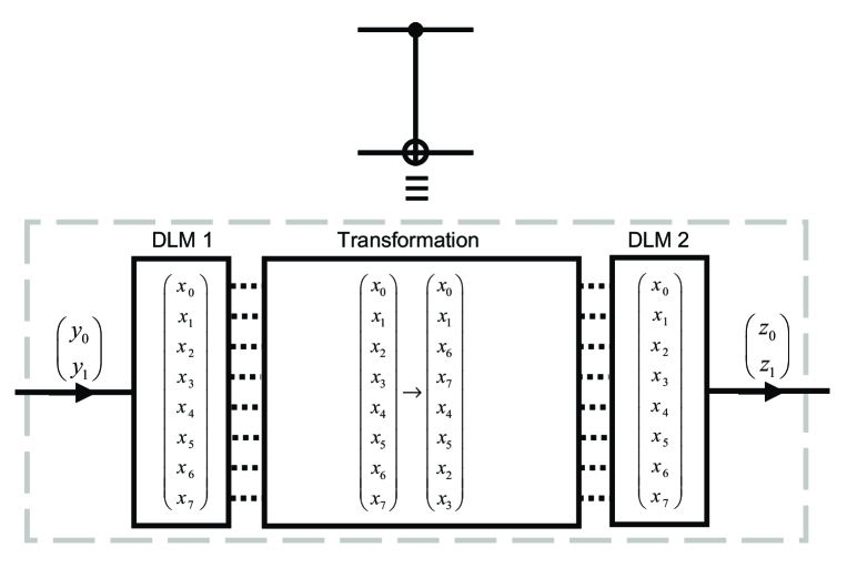
Figure 7: Diagram of a DLM-based processor that simulates a CNOT gate on an event-by-event basis.

Instead of presenting results that show that the DLM-processor of Fig. 7 correctly performs the CNOT operation on an event-by-event basis, we consider the more complicated network of four Hadamard gates and one CNOT gate shown in Fig. 3. Quantum mechanically, this network acts as a CNOT gate in which the role of control- and target qubit have been interchanged NIEL00 . For this DLM-network to perform correctly it is essential that the event-based simulation mimics the quantum interference (generated by the Hadamard gates) correctly. In Table 2 we present simulation results for the DLM-network shown in Fig. 3. Before the simulation starts, we use uniform random numbers to initialize the internal vectors of the DLMs (ten vectors in total). For simplicity, we take as input messages $\phi_{0}=\phi_{1}=\phi_{2}=\phi_{3}=0$. All these simulations were carried out with $\alpha=0.99$. From Table 2 it is clear that, also for a modest number of input events, the network reproduces the results of the corresponding quantum circuit, i.e. a CNOT operation in which qubit 2 is the control qubit and qubit 1 is the target qubit NIEL00 .

Table 2: Simulation results for the DLM-network shown in Fig. 3, demonstrating that the network reproduces the results of the corresponding quantum circuit, i.e. a CNOT operation in which qubit 2 is the control qubit and qubit 1 is the target qubit NIEL00 . The first half of the events are discarded in the calculation of the frequency $f_{i}$ for observing an output event of type $i=0,1,2,3$, corresponding to the probability to observe the quantum system in the state $|00\rangle$, $|01\rangle$, $|10\rangle$, or $|11\rangle$, respectively. For 200 events or more, the difference between the event-based simulation results and the corresponding quantum mechanical probabilities is less than 1%.

Number of events	Qubit 1	Qubit 2	$f_{0}$	$f_{1}$	$f_{2}$	$f_{3}$
100	0	0	$0.98$	$0.00$	$0.00$	$0.02$
100	1	0	$0.20$	$0.74$	$0.01$	$0.04$
100	0	1	$0.16$	$0.04$	$0.00$	$0.80$
100	1	1	$0.16$	$0.04$	$0.72$	$0.08$
200	0	0	$1.00$	$0.00$	$0.00$	$0.00$
200	1	0	$0.00$	$1.00$	$0.00$	$0.00$
200	0	1	$0.00$	$0.00$	$0.00$	$1.00$
200	1	1	$0.01$	$0.00$	$0.99$	$0.00$

As an illustration of the use of SLMs, we replace all the back-end DLMs in the CNOT circuit shown in Fig. 7 by SLMs. and repeat the simulations that yield the data in Table 2. From Table 3 we conclude that the randomized version generates the correct results but significantly more events are needed to achieve similar accuracy as in the fully deterministic simulation.

Table 3: Simulation results for the DLM-network shown in Fig. 3 in which each back-end DLM of the individual gates has been replaced by a SLM. The latter uses random numbers to randomize the order in which different output events are generated but does not change the frequencies of the events. The first half of the input events are discarded for the calculation of the frequencies $f_{i}$ for observing an output event of type $i=0,1,2,3$, corresponding to the probability to observe the quantum system in the state $|00\rangle$, $|01\rangle$, $|10\rangle$, or $|11\rangle$, respectively.

Number of events	Qubit 1	Qubit 2	$f_{0}$	$f_{1}$	$f_{2}$	$f_{3}$
2000	0	0	$0.965$	$0.015$	$0.010$	$0.010$
2000	1	0	$0.007$	$0.970$	$0.012$	$0.011$
2000	0	1	$0.010$	$0.008$	$0.016$	$0.966$
2000	1	1	$0.005$	$0.016$	$0.963$	$0.016$

IV.4 Number factoring

Finally, we discuss the results obtained by a DLM-based simulation of the number factoring circuits depicted in Fig. 4. DLM networks (not shown) that perform the Toffoli gate operation and the Fourier transform, which involves several Hadamard operations and controlled phase shifts, are readily constructed by mimicking the procedure for the construction of the DLM network of the CNOT gate. Having done this, building the circuit in Fig. 4 entails nothing than connecting the DLM networks that simulate the various quantum gates. As this circuit involves seven qubits, the internal vectors of the DLMs have 256 elements.

Section II.5 shows that if $a=7$, we expect to find $Q_{1}=\langle Q_{1}^{z}\rangle=0$, $Q_{2}=\langle Q_{2}^{z}\rangle=0.5$, and $Q_{3}=\langle Q_{3}^{z}\rangle=0.5$. Similarly, for $a=11$ we expect to find $Q_{1}=\langle Q_{1}^{z}\rangle=0$, $Q_{2}=\langle Q_{2}^{z}\rangle=0$, and $Q_{3}=\langle Q_{3}^{z}\rangle=0.5$. In the DLM approach, simply counting the number of 1 events in the three output channels of the Fourier transform (inside the dashed box in Fig. 4) and dividing these numbers by the total number of events analyzed, we obtain numerical estimates for the qubits $Q_{1}=\langle Q_{1}^{z}\rangle$, $Q_{2}=\langle Q_{2}^{z}\rangle$, and $Q_{3}=\langle Q_{3}^{z}\rangle$. In Figs. 8-11 we present simulation results for the DLM (left panel) and SLM (right panel) implementation of the circuit depicted in Fig. 4, for the two cases $a=7,11$ and for two choices of the control parameter $\alpha=0.99,0.999$. After processing a few events, (less than 200 if $\alpha=0.99$ less than 2000 if $\alpha=0.999$) all the DLM networks reproduce the results of quantum theory with high accuracy. Replacing DLMs by their stochastic equivalents (SLMs), we see that the fluctuations are larger than if we use DLMs and that the system as a whole “learns” much slower. This is to be expected: the probabilistic mechanism to distribute events over the output channels of the SLMs makes much more “mistakes” than the deterministic process used by the DLMs. DLMs encode the information about the probability and phase in a much more effective, compact manner than SLMs. In the case of the latter, the correct probability distribution is encoded in a statistical manner and can only be recovered by analyzing a lot of events.

From the description of the learning process, it is clear that $\alpha$ controls the rate of learning or, equivalently, the rate at which learned information can be forgotten. Furthermore it is evident that the difference between a constant input to a DLM and the learned value of its internal variable cannot be smaller than $1-\alpha$. In other words, $\alpha$ also limits the precision with which the internal variable can represent a sequence of constant input values. On the other hand, the number of events has to balance the rate at which the DLM can forget a learned input value. The smaller $1-\alpha$ is, the larger the number of events has to be for the DLM to adapt to changes in the input data. The results depicted in Figs. 8-9 and Figs. 10-11 confirm this behavior.

Figure 8: Event-by-event simulation of Shor’s quantum algorithm for factoring the integer $N=15$, using the value $a=7$ (see Section II.5). Each data point represents the average of 100 output events. The parameter that controls the learning process of the DLMs is $\alpha=0.99$. Left: Deterministic simulation employing DLMs. Right: Stochastic simulation employing SLMs.

Figure 9: Same as Fig. 8, except that $a=11$ (see Section II.5).

Figure 10: Event-by-event simulation of Shor’s quantum algorithm for factoring the integer $N=15$, using the value $a=7$ (see Section II.5). Each data point represents the average of 100 output events. The parameter that controls the learning process of the DLMs is $\alpha=0.999$. Left: Deterministic simulation employing DLMs. Right: Stochastic simulation employing SLMs.

Figure 11: Same as Fig. 10, except that $a=11$ (see Section II.5).

V Discussion

We have shown that locally connected networks of machines that have primitive learning capabilities can be used to perform a deterministic, event-based simulation of quantum computation. On the other hand it is known that the time evolution of the wave function of a quantum system can be simulated on a quantum computer ZALK98 ; NIEL00 . Therefore, it is possible to simulate real-time quantum dynamics through a deterministic event-based simulation by constructing appropriate DLM-networks. The work presented in this paper suggests that there exist deterministic, particle-like processes that reproduce quantum mechanical behavior.

Just as any other method for simulating quantum computers RAED05 , the DLM-based simulation approach requires memory resources that increase exponentially with the number of qubits. This exponential increase is merely a combinatorial effect and is not at all related to the quantum nature of the phenomena we want to simulate. As a matter of fact, it is present in all classical or quantum many-body systems (including quantum computers). For instance, if we consider one of the most basic statistical mechanics models, the Ising model, the number of possible states of this system also grows exponentially with the number of spins but there obviously is nothing “quantum” about this model.

The computational efficiency of the event-based approach is lower than the efficiency of algorithms that directly compute the product of the unitary matrices. This is hardly a surprise: The former approach simulates quantum behavior by generating individual events. The latter can only simulate the outcome of (infinitely) many of such events and provides no information about individual events HOME97 . An analogy may be helpful to understand the conceptual difference between these two approaches. It is well known that an ensemble of simple, symmetric random walks may be approximated by a diffusion equation (for vanishing lattice spacing and time step). Also here we have two options. If we are interested in individual events, we have no other choice than to simulate the discrete random walk. However, if we want to study the behavior of many random walkers, it is computationally much more efficient to solve the corresponding diffusion problem.

Our event-based approach can be extended to mimic the effects of decoherence. In quantum theory, decoherence causes the loss of phase coherence ZURE03 . In the DLMs that we describe in Section IV, a single parameter ($\alpha$) controls the loss of memory, of both the probability and the phase. A simple extension would be to control the learning process of the probability and phase separately, using two control parameters. We leave this topic for future research.

References

- (1) I. Chiorescu, P. Bertet, K. Semba, Y. Nakamura, C.J.P.M. Harmans, and J.E. Mooij, Nature 431, 159 (2004)
- (2) D. Rugar, R. Budakian, H.J. Mamin, and B.W. Chui, Nature 430, 329 (2004)
- (3) J.M. Elzerman, R. Hanson, L.H. Willems van Beveren, B. Witkamp, L.M.K. Vandersypen, and L.P. Kouwenhoven, Nature 435, 331 (2004)
- (4) X. Xiao, I. Martin, E. Yablonovitch, and H.W. Jiang, Nature 435, 335 (2004)
- (5) T. Fujisawa, NTT Technical Review 1, 41 (2003)
- (6) M. Nielsen and I. Chuang, Quantum Computation and Quantum Information, Cambridge University Press, Cambridge (2000)
- (7) R.P. Feynman, R.B. Leighton, M. Sands, The Feynman lectures on Physics, Addison-Wesley, Reading MA (1996), Vol. 3
- (8) D. Home, Conceptual Foundations of Quantum Physics, Plenum Press, New York (1997)
- (9) A. Tonomura, The Quantum World Unveiled by Electron Waves, World Scientific, Singapore (1998)
- (10) L.E. Ballentine, Quantum Mechanics: A Modern Development, World Scientific, Singapore (2003)
- (11) R. Penrose, The Emperor’s New Mind, Oxford University Press, Oxford (1990)
- (12) In this paper we disregard limitations of real experiments such as detector efficiency, imperfection of the source, biprism and the like.
- (13) P. Grangier, R. Roger, and A. Aspect, Europhys. Lett. 1, 173 (1986)
- (14) N.G. Van Kampen, Physica A 153, 97 (1988)
- (15) K. De Raedt, H. De Raedt, and K. Michielsen, http://arxiv.org/abs/quant-ph/0409213
- (16) P.W. Shor, SIAM Review 41, 303 (1999)
- (17) S. Haykin, Neural Networks, Prentice Hall, New Jersey (1999)
- (18) L.I. Schiff, Quantum Mechanics, McGraw-Hill, New York (1968)
- (19) G. Baym, Lectures on Quantum Mechanics, W.A. Benjamin, Reading MA (1974)
- (20) We make a distinction between quantum theory and quantum physics. We use the term quantum theory when we refer to the mathematical formalism, i.e., the postulates of quantum mechanics (with or without the wave function collapse postulate) BALL03 and the rules (algorithms) to compute the wave function. The term quantum physics is used for microscopic, experimentally observable phenomena that do not find an explanation within the mathematical framework of classical mechanics.
- (21) D.P. DiVincenzo, Phys. Rev. A51, 1015 (1995)
- (22) M. Born and E. Wolf, Principles of Optics, Pergamon, Oxford (1964)
- (23) J.G. Rarity and P.R. Tapster, Phil. Trans. R. Soc. Lond. A 355, 2267 (1997)
- (24) A. Barenco, C.H. Bennett, R. Cleve, D.P. DiVincenzo, N. Margolus, P. Shor, T. Sleator, J.A. Smolin, and H. Weinfurter, Phys. Rev. A52, 3457 (1995)
- (25) L.M.K. Vandersypen, http://arxiv.org/abs/quant-ph/0205193 (URL last accessed on July 29, 2004)
- (26) L.M.K. Vandersypen, M. Steffen, G. Breyta, C.S. Yannoni, M.H. Sherwood, and I.L. Chuang, Nature 414, 883 (2001)
- (27) A. Ekert and R. Jozsa, Rev. Mod. Phys. 68, 733 (1996)
- (28) H. De Raedt, A.H. Hams, K. Michielsen, and K. De Raedt, Comp. Phys. Comm. 132, 1 (2000)
- (29) K.F.L. Michielsen and H. De Raedt, Turk. J. Phys. 27, 343 (2003)
- (30) H. De Raedt and K. Michielsen, in Handbook of Computational and Theoretical Nanotechnology, Edited by M. Rieth and W. Schommers, American Scientific Publisher, Los Angeles (2005), in press
- (31) QCE can be downloaded from http:/www.compphys.org/qce.htm (URL last accessed on November 23, 2004)
- (32) A large collection of video’s of such simulations can be found at http://www.compphys.org/quantummechanics (URL last accessed on November 23, 2004)
- (33) H. De Raedt, K. De Raedt, and K. Michielsen, J. Phys. Soc. Jpn. (in press)
- (34) Interactive programs that performs the event-based simulations of a beam splitter, one Mach-Zehnder interferometer, and two chained Mach-Zehnder interferometers can be found at http://www.compphys.net/dlm (URL last accessed on November 23, 2004)
- (35) C. Zalka, Proc. R. Soc. Lond. A454, 313 (1998)
- (36) W.H. Zurek, Rev. Mod. Phys. 75, 715 (2003)