Exact quantization of nonsolvable potentials: the role of the quantum phase beyond the semiclassical approximation

Abstract

Semiclassical quantization is exact only for the so called solvable potentials, such as the harmonic oscillator. In the nonsolvable case the semiclassical phase, given by a series in $\hbar$, yields more or less approximate results and eventually diverges due to the asymptotic nature of the expansion. A quantum phase is derived to bypass these shortcomings. It achieves exact quantization of nonsolvable potentials and allows to obtain the quantum wavefunction while locally approaching the best pre-divergent semiclassical expansion. An iterative procedure allowing to implement practical calculations with a modest computational cost is also given. The theory is illustrated on two examples for which the limitations of the semiclassical approach were recently highlighted: cold atomic collisions and anharmonic oscillators in the nonperturbative regime.

The semiclassical treatment of integrable systems, which can be traced back to Bohr’s atomic model of planetary motion and Einstein’s classic paper on the quantization of regular motion bohr-einstein is assumed to be a well-established and venerable subject. It is true that WKB theory, where the phase to be quantized is the classical action, can be found in any standard textbook, but WKB often results in approximations that are quantitatively too crude and that fail to capture the physics of the problem. Indeed, WKB theory achieves exact quantization for a restricted number of potentials - known as the solvable potentials - such as the harmonic and Morse oscillators or the centrifugal Coulomb problem. In the last decade, the application of supersymmetric (SUSY) methods to quantum mechanics has enlarged this list to a handful of other potentials, quantized by employing SUSY WKB sukhatme97 . However, even in the solvable cases, the WKB wavefunctions are innaccurate especially at the turning points where they blow up, and a consistent divergence-free WKB scheme is still a topic of current investigation divfree2002 . In the more general nonsolvable case, WKB quantization has frequently resulted in useful approximations to compute the energy levels of excited states, but recently several shortcomings were pointed out: for example the phase loss in the classically forbidden regions is badly taken into account by WKB theory in potentials used in atomic clusters calculations friedrich96 ; in cold atom collisions WKB quantization breaks down for very excited states boisseau98 ; for anharmonic potentials, the failure of WKB has prompted extensive developments of numerically involved quantum techniques with the aim of obtaining accurate results hatsuda97 ; meissner97 for applications ranging from molecular physics to quantum field theories.

We show in this work that these shortcomings can be resolved by considering an exact quantum phase. Although the quantum phase bears a very close relationship to the semiclassical one, it is necessary to go beyond the semiclassical approach in the presence of nonsolvable potentials. Indeed, the failure of the semiclassical approximation resides in the limitations imposed by the underlying classical dynamics. Let us take a one dimensional conservative system at energy $E$, which will be our main concern in this work. The WKB wavefunction is built from blocks given by brack badhuri

$$\psi_{\mathrm{WKB}}(x,E)=A(x,E)\exp[iS(x,E)/\hbar]$$ (1)

where the phase function $S(x,E)$ is the classical action and $A^{2}(x,E)=(\partial_{x}S)^{-1}$ gives the classical probability amplitude. The WKB quantization condition reads

$$S(t_{2},E)-S(t_{1},E)=\left(n+\frac{\mu}{4}\right)\pi\hbar,$$ (2)

where $t_{1,2}$ are the turning points, $\mu$ is the Maslov index (generally 2 in one dimensional systems) and $n$ is the level integer. To improve the approximation a semiclassical expansion going beyond these purely classical terms can be carried out by going to higher order in $\hbar$. However this expansion is an asymptotic series, which means that although going to higher order may improve the accuracy of the results, at some point the series generally diverge bender77-voros93 . Moreover the divergence of the amplitude at the turning points becomes worse at each order and regularization techniques are needed to compute the phase integrals.

This is why a quantum phase $\sigma(x,E)$ while implicitly summing the divergent semiclassical expansion needs to be defined from the start by appropriately transforming the Schrödinger equation

$$\hbar^{2}\partial_{x}^{2}y(x)+p^{2}(x)y(x)=0,$$ (3)

where $p(x)$ is the classical momentum. A transformation of the Liouville-Green type slavyanov96 is taken by writing

$$y(x)=\left(\partial_{x}\xi(x)\right)^{-1/2}w(\xi),$$ (4)

so that $\xi(x)$ appears as a ’phase’ and the prefactor as an amplitude, as in Eq. (1). Assume $w(\xi)$ fulfills the equation

$$\hbar^{2}\partial_{\xi}^{2}w(\xi)+R(\xi)w(\xi)=0,$$ (5)

where the choice of the unspecified function $R(\xi)$ determines the choice of $w$. $\xi$ then obeys

$$R(\xi)\left(\partial_{x}\xi\right)^{2}-p^{2}(x)+\frac{\hbar^{2}}{2}\left\langle\xi;x\right\rangle=0,$$ (6)

where $\left\langle\xi;x\right\rangle\equiv\partial_{x}^{3}\xi/\partial_{x}\xi-\frac{3}{2}(\partial_{x}^{2}\xi/\partial_{x}\xi)^{2}$ denotes the Schwartzian derivative. We thus see that the choice of the phase first depends on the choice of the carrier function $w$ (or equivalently, of $R(\xi)$), and then on the choice of the boundary conditions that need to be imposed on the third order nonlinear Eq. (6). This is an illustration of the ambiguity suffered by phase functions in quantum mechanics, due here to the fact that there is no unique manner to cut a given wavefunction into a phase $\xi$ on the one hand, and an amplitude function obeying the continuity equation $\alpha(x,E)=(\partial_{x}\xi)^{-1/2}$ (as in the semiclassical case) on the other.

Formally $\xi(x)$ can be expanded as an asymptotic series in $\hbar$ irrespective of the specific choice of $R$. It is nevertheless apparent from Eq. (6) that the only choice that will give $\xi(x)\sim S(x)$ to first order in $\hbar$ corresponds to $R(\xi)=\pm 1$, leading by Eq. (5) to circular or exponential carrier functions. The price to pay is that the $\hbar$ expansion based on these functions – such as the WKB approximation, necessarily diverges at the turning points. However the exact solution of Eq. (6) does not present such deficiencies, pointing to the possibility of defining a quantum phase from Eq. (6) with $R(\xi)=\pm 1$. For bound state problems the solutions of Eq. (3) are real so $w$ can be taken as a circular function. $y(x)$ then becomes proportional to $\alpha(x)\sin\sigma(x),$ with $\sigma$ denoting the phase $\xi$ when $R=\pm 1$. Let $p(x)$ span the interval $]s_{1},s_{2}[$ (typically $]-\infty,+\infty[$ or $]0,+\infty[$ for radial problems). It can then be shown matzkin01 that $\alpha$ is a positive definite quadratic form that behaves as $\alpha(x\rightarrow s_{i=1,2})\rightarrow\infty$ so that setting $\sigma(s_{1})=0$ the quantization condition reads

$$\sigma(s_{2},E)=(n+1)\pi,$$ (7)

where $n$ is the level integer as in Eq. (2). Eq. (7) is exact and holds irrespective of the boundary conditions imposed on $\sigma$.

For computational purposes, Eq. (6) is intricate to solve. It can be checked that by writing (we use atomic units and assume $R(\xi)=1$ from now on)

$$M(x,E)=\partial_{x}\left[\sigma(x,E)+\frac{i}{2}\ln(\partial_{x}\sigma)\right],$$ (8)

Eq. (6) leads to the complex but first order nonlinear differential equation

$$\partial_{x}M=i\left(p^{2}(x)-M^{2}(x)\right)\equiv\mathcal{F}(M(x),x),$$ (9)

where $\mathcal{F}$ denotes the middle term taken as a functional. Our strategy will consist in solving the equation for $M$; the real part will give us $\partial_{x}\sigma,$ which can be numerically integrated to obtain $\sigma,$ yielding both the wavefunction and the total phase $\sigma(s_{2},E)$. To do so we first linearize the equation for $M$ by expanding the functional to first order in the vicinity of an initial trial function $M_{0}(x)$. We then solve

$$\partial_{x}M_{q+1}=\mathcal{F}(M_{q}(x),x)+\left.\frac{\delta\mathcal{F}}{\delta M}\right|_{M_{q}}\left(M_{q+1}(x)-M_{q}(x)\right),$$ (10)

with $q=0$ and where $\delta$ stands for the functional derivative. Eq. (10) is a linear first order differential equation that can be solved straighforwardly. Of course since $\mathcal{F}$ has been linearized Eq. (10) is not equivalent to Eq. (9), hence the subscript in $M_{1}$. Convergence towards $M$ is achieved by iterating the procedure, i.e. we now solve Eq. (10) for $q=1,$ obtaining a better approximation $M_{2}$ and so on. This iterative linearization procedure, known as the quasilinearization method (QLM) replaces the solution of a nonlinear differential equation by iteratively solving a linear one. It was introduced 3 decades ago by Bellman and Kalaba bellman in the context of linear programming, but the extension of QLM to the type of functions dealt with in quantum mechanics is quite recent mandelzweig99 . In particular, the property of quadratic convergence which makes this method powerful still holds. Indeed, 5 to 6 iterations typically suffice to obtain solutions with high precision (e.g. more than 20 decimal digits).

To iteratively solve Eq. (10), two ingredients are needed: first the trial function $M_{0}(x)$, second, the boundary condition, $M_{q}(x_{b})$ which is set from the start since it must be the same for each $q$. The choice of $M_{0}$ is actually unimportant, since any sufficiently well behaved trial function, i.e. behaving as $\left|p(x)\right|$ between the turning points and as $i\left|p(x)\right|$ (resp. $-i\left|p(x)\right|$) for $x<t_{1}$ (resp. $x>t_{2}$), with a smooth transition between the regions, will lead to the same converged answer. An elegant solution consists in determining the first order semiclassical expression not diverging at the turning points, which is done by appropriately choosing $R(\xi)$ in Eq. (5) and expressing $\sigma$ in terms of $\xi_{R\neq 1},$ but we shall not pursue this task here matzkin-prep . What is crucial is the choice of the boundary condition because it determines the behavior of the solution. We draw here on previous work where we had shown that if $\sigma(x)$ is written as an infinite $\hbar$ expansion, there is a unique boundary condition that yields the classical action $S(x)$ when the limit $\hbar\rightarrow 0$ is taken matzkin01 . For other boundary conditions, the limit $\hbar\rightarrow 0$ yields a semiclassical phase (and the corresponding amplitude) that displays the oscillations of the WKB wavefunction. The existence of an optimal boundary condition is well known in the context of solvable potentials, where the use of analytic solutions (e.g. parabolic cylinder functions for the harmonic oscillator, Whittaker functions in the centrifugal Coulomb case seaton83 ) allows to explicitly construct a nonoscillating quantum phase. However for nonsolvable potentials a procedure based on special functions does not exist, whereas the $\hbar$ expansions employed in matzkin01 are of formal nature. To ensure that the quantum phase behaves as the $\hbar$ expansion would if it converged arnold , we choose here the simplest solution, namely to pick an appropriate point $x_{b}$ in the classically allowed region where the standard  ($R(\xi)=1$) semiclassical expansion can be employed and go to the highest possible order in $\hbar$ before the series starts to diverge. More refined methods of estimating the optimal boundary condition, based on super and hyper-asymptotic expansions boyd , are in principle available, but they are unnecessary insofar as neither the behavior of $\sigma$ nor the quantum mechanical quantities would be affected by their use.

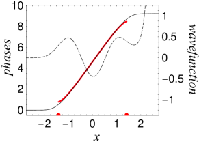
Figure 1: Left scale: The quantum phase $\sigma(x)$ (solid black curve) for the anharmonic oscillator at $E=5$ (units in a.u.) shown along with the classical action $S(x)$ (thick gray/red curve) plotted between the turning points (semicircles on the $x$ axis). Note that we have taken $S(t_{1})=\pi/4$. This $\pi/4$ constant is familiar from standard WKB analysis brack badhuri but it can also be rigorously proved slavyanov96 ; matzkin-prep that the semiclassical phase not diverging at the turning points, obtained from Eq. (6) with $R(\xi)=\xi$, behaves as $\sigma_{scl}(x)\backsimeq S(x)/\hbar+\pi/4$ for $x\gg t_{1}$ (but $\sigma_{scl}(t_{1})=\pi/6$). Right scale: The associated wavefunction $\alpha\sin\sigma$. Since $E$ is not an eigenvalue this improper wavefunction is normalized per unit energy, as usual in scattering theory.

We will now illustrate and detail the properties of the quantum phase on two specific examples. The first example concerns anharmonic oscillators which are employed in the investigation of quite different phenomena, ranging from molecular vibrations to quantum field theories and phase transitions. This has generated different schemes to compute the eigenvalues and the wavefunctions, calling for large numerical basis macfarlane-annphys ; meissner97 or delicate resummation techniques hatsuda97 . The failure of the semiclassical approximation which is important for the lowest levels (e.g., for symmetric potentials $x^{2m}$ WKB quantization gives the wrong behavior of the energies as a function of $m$) but persists for more excited states, has been generally attributed to the existence of complex turning points away from the real line chebotarev99 . However the complex plane does not play directly any rôle in the present scheme, based on the construction of a real quantum phase. Fig. 1 shows the quantum phase $\sigma(x,E)$ along with the classical action for a Hamiltonian with an anharmonic potential $x^{2}+2x^{4}$. Given the symmetry of the potential, we have taken $x_{b}=0$ and fixed the value $M_{0}(x_{b})$ by carrying out a semiclassical expansion up to $o(h^{14})$. We have also plotted on the same figure the associated wavefunction. It diverges beyond the right turning point because we have voluntarily chosen $E$ not to be an eigenvalue (here $E$ lies between the 2nd and the 3rd levels). The bound states are found by applying the quantization condition (7) in the following way: the total phase $\sigma(s_{2},E)$ at $s_{2}=\infty$ is determined for different values of the energy (the energy grid can be more or less sparse, depending on the required numerical precision). The points are then interpolated to yield the curve $\sigma(s_{2},E)$ as a function of $E$ seen on Fig. 2, which allows to solve for $E$ in Eq. (7). By that method we have determined the ground and the first 35 states of this anharmonic oscillator and compared the eigenenergies to the precise quantum calculations of meissner97 , obtaining exactly the same results as those published in their Table III.

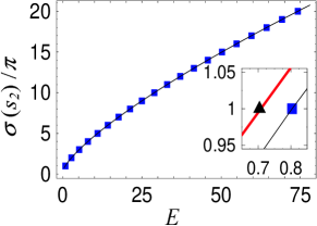
Figure 2: Energy levels of the anharmonic oscillator (a.u.) obtained by quantizing the quantum phase. The smooth curve represents $\sigma(s_{2},E)/\pi$ as a function of the energy and the boxes are plotted each time this quantity equals the integer $n+1$, determining the exact levels (here the first 20 levels $n=0-19$ are plotted). The inset zooms on the ground state: the thick gray/red line gives the semiclassical quantization curve $(S(t_{2},E)-S(t_{1},E))/\pi+1/2$ (the $\hbar$ expansion diverges beyond this order) and the triangle the semiclassically quantized level, which is off by more than 10%.

The second illustration involves a potential well with a strong repulsion at short-range and a long-range attractive tail. This type of potential is of interest in the study of cold atomic collisions, a field that has been sparked by the development of photoassociative spectroscopy boisseau98 . The WKB approximation breaks down for excited states near the threshhold, a fact that is hardly surprising since it is understood that WKB may fail when the quantum particle explores large areas of classically forbidden regionsfriedrich04 . We take the following 12-6 Lennard-Jones (LJ) potential with the classical momentum given in the scaled form as

$$p^{2}(x)=B\left[E-\left(\frac{1}{x^{12}}-\frac{2}{x^{6}}\right)\right]$$ (11)

where $B$ is a ’strength’ parameter. This potential with $B=10^{4}$ has often been employed as a benchmark (see leroy83-boisseau00 ; friedrich04 and Refs. therein) and is known to support 24 states. The WKB quantization condition (2) gives energies with an error relative to the local level spacing that globally increases with $E$. Fig. 3 compares the derivative of the quantum phase $\partial_{x}\sigma(x,E)$ with the classical momentum $\partial_{x}S(x,E)$ for the last bound state just below the threshold. $x_{b}$ was taken to the right of the potential minimum and the $\hbar$ expansion was carried out up to the 12th order. The 2 curves are barely distinguishable in the classically allowed region, so we have focused on the zone near the turning points. Note that the quantum curve largely penetrates into the classically forbidden region well beyond the outer turning point. This is typical of excited states in potentials with a long-range attractive tail and can be seen as the underlying reason ruling the breakdown of the semiclassical approximation. Quantization proceeds as in the first example, by determining $\sigma(s_{2},E)$ on an energy grid then solving for Eq. (7). The resulting curve is shown in Fig. 4 and the quantized energies of the 24 levels exactly reproduce the values of exact quantum mechanical calculations friedrich04 . In particular the position of the last level determines the scattering length, a crucial parameter in the production of Bose-Einstein condensates.

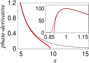
Figure 3: Derivative of the quantum phase $\partial_{x}\sigma$ (solid black curve) and of the classical action $\partial_{x}S=p$ (thick gray/red curve) in the 12-6 LJ potential characteristic of cold atom collisions (scaled a. u.). These quantities, plotted for the most excited bound state, are shown in the zone near the outer turning point $t_{2}\thickapprox 9.5$. The inset shows the zone near the inner turning point $t_{1}\thickapprox 0.9$ (note the very different scales).

To summarize, we have employed a quantum phase that goes beyond the semiclassical approximation in giving the exact quantization energies as well as the wavefunctions. We have also given a numerical procedure to determine the phase based on the linearization of the phase equation and a boundary condition obtained from a local semiclassical expansion, and illustrated the approach in the case of two nonsolvable potentials.

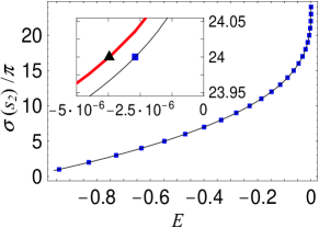
Figure 4: Exact energy levels (boxes) of the 12-6 LJ potential obtained by quantizing $\sigma(s_{2},E)$ (solid curve), in scaled a.u. The inset zooms on the last state below threshold ($E=0$) and also shows the WKB prediction, about 40% too low (triangle).

References

- (1) N. Bohr, Phil. Mag. 26, 1 (1913). A. Einstein, Vehr. Deutsch. Phys. Ges. Berlin 19, 82 (1917).
- (2) M. Hruska, W.Y. Keung and U. Sukhatme, Phys. Rev. A 55, 3345 (1997).
- (3) T. Hyouguchi, R. Seto, M. Ueda and S. Adachi, Ann. Phys. 312, 177 (2004).
- (4) H. Friedrich and J. Trost, Phys. Rev. A 54, 1136 (1996).
- (5) C. Boisseau, E. Audouard and J. Vigue, Europhys. Lett. 41, 349 (1998).
- (6) T. Hatsuda, T. Kunihiro and T. Tanaka, Phys. Rev. Lett. 78, 3229 (1997).
- (7) H. Meissner and E. O. Steinborn, Phys. Rev. A 56, 1189(1997).
- (8) M. Brack and R. Bhaduri, Semiclassical Physics (Addison Wesley, Reading, 1997).
- (9) C. M. Bender, K. Olaussen and P. S. Wang, Phys. Rev. D 16, 1740 (1977). A. Voros, Ann. I Fourier 43, 1509 (1993).
- (10) S. Yu. Slavyanov, Asymptotic Solutions of the One-Dimensional Schrodinger Equation (AMS, Providence (RI), 1996).
- (11) A. Matzkin, J. Phys. A 34, 7833 (2001).
- (12) R. E. Bellman and R. Kalaba, Quasilinearization and nonlinear boundary-value problems (Elsevier, New York, 1965).
- (13) V. B. Mandelzweig, J. Math. Phys. 40, 6266 (1999). R. Krivec and V. B. Mandelzweig, Comput. Phys. Comm. 152, 165 (2003).
- (14) A. Matzkin, in preparation.
- (15) M. J. Seaton, Rep. Prog. Phys. 46, 167 (1983).
- (16) As put by Arnold (in Mathematical Methods of Classical Mechanics (Springer, Berlin, 1989)), the divergence of the series means that ’we are looking for an object that does not exist’ as an expansion.
- (17) J. P. Boyd, Acta Appl. Math. 56, 1 (1999).
- (18) M. H. Macfarlane, Ann. Phys. 271, 159 (1999).
- (19) L. V. Chebotarev, Ann. Phys. 273, 114 (1999).
- (20) H. Friedrich and J. Trost, Phys. Rep. 397, 359 (2004).
- (21) C. Boisseau, E. Audouard, J. Vigue and V. V. Flambaum, Eur. Phys. J. D 12, 199 (2000).