Multimode entanglement of light and atomic ensembles via off-resonant coherent forward scattering

Abstract

Quantum theoretical treatment of coherent forward scattering of light in a polarized atomic ensemble with an arbitrary angular momentum is developed. We consider coherent forward scattering of a weak radiation field interacting with a realistic multi-level atomic transition. Based on the concept of an effective Hamiltonian and on the Heisenberg formalism, we discuss the coupled dynamics of the quantum fluctuations of the polarization Stokes components of propagating light and of the collective spin fluctuations of the scattering atoms. We show that in the process of coherent forward scattering this dynamics can be described in terms of a polariton-type spin wave created in the atomic sample. Our work presents a general example of entangling process in the system of collective quantum states of light and atomic angular momenta, previously considered only for the case of spin $\small{1/2}$ atoms. We use the developed general formalism to test the applicability of spin $\small{1/2}$ approximation for modelling the quantum non-demolishing measurement of atoms with a higher angular momentum.

I Introduction

Various optical phenomena associated with the optical pumping process, which have been comprehensively studied since the 60’s and described in many aspects in a famous review Hpr by W.Happer, is revived nowadays in a new form within the field of quantum information and quantum computing. The paramagnetic ground states of macroscopic atomic spin subsystems are considered now convenient physical objects for mapping and storing the quantum information in the quantum states of their collective angular momenta. The Faraday-type interference scheme was proposed for spin squeezing K1 and for quantum communication between atomic ensembles DCZP . The proposed ideas were realized in spin squeezing K2 and in the entanglement JKP experiments, where a quantum measurement on the light forward-scattered from atomic ensembles was used. The same kind of off-resonant forward scattering combined with a quantum feedback was used in the recent demonstration of quantum memory for light H . Applications to various quantum information protocols including a cat state generation J and quantum cloning of light onto atoms cloning have been proposed. Efficient generation of entanglement via multi-pass interaction have been also proposed Polzik . Theoretical modelling in the above mentioned papers was concerned with collective canonical variables for atoms which can be conveniently introduced for spin $\small{1/2}$ atoms. However, the actual experiments were conducted using states with higher angular momenta. Hence a theoretical model describing off-resonant interaction of light with realistic atoms with the angular momentum higher then $\small{1/2}$ is required.

It is worth noting that the effect of a random Faraday rotation due to atomic fluctuations was discussed and observed first in Refs.AlZp ; GlPl more than twenty years ago in the context of demonstrating the advantages of light-beating method in atomic spectroscopy. The importance of atomic polarization was later discussed in Refs.KpSk ; BKS where it was shown that the collective spin polarization of an atomic ensemble could essentially modify the quantum statistics of the outgoing off-resonant probe radiation. Quantum statistics of atomic spin variables was first experimentally observed via off-resonant forward scattering in Hald .

In the present paper we develop the quantum theory of coherent forward scattering on an ensemble of polarized atoms with an arbitrary angular momentum. We discuss the physical conditions under which the forward scattering can be properly described in terms of the effective Hamiltonian, generalizing the semiclassical approach Hpr , so that both the field and atomic subsystems are treated as quantum objects. Based on the effective Hamiltonian we derive the Heisenberg-type equations of motion written for the spatial distribution of the Stokes variables of the field and of the collective angular momentum of atoms. The solution shows how the entanglement of the quantum fluctuations of light and atomic subsystems is formed. We show that the entangling process can be understood in terms of a polariton-type spin wave induced in the atomic sample. We support our discussion by numerical simulations, assuming the conditions close to those of the recent experiments JKP .

The paper is organized as follows. In section II we review the process of coherent forward scattering to show how the field Heisenberg operators are transformed in interaction with multi-atom ensemble consisting of atoms with an arbitrary Zeeman structure and for an off-resonant excitation on a dipole allowed optical transition. In section III we extend the Heisenberg formalism to the atomic subsystem and introduce the effective Hamiltonian responsible for the coupled dynamics of an infinite number of variables associated with the local polarization of the weak probe light and with individual atomic spins. The effective Hamiltonian is further transformed in section IV into another form by introducing the more convenient for the polarization sensitive processes irreducible tensor formalism. In section V we perform mesoscopic averaging to arrive at the wave-type equations for the collective quantum variables of the light and atomic subsystems. These equations are solved and discussed in section VI in the context of the quantum entangling process. In particular they are used to test the applicability of the spin one-half approximation for modelling the quantum non-demolishing measurement in an ensemble of alkali atoms with a higher angular momentum.

II Coherent forward scattering of light in the Heisenberg picture

Consider a system of $N$ identical atoms located in a finite volume and scattering coherent light of frequency $\omega$. The wave of light incident on the atomic ensemble is assumed to be weak enough that possible saturation effects in its interaction with the atoms are negligible. The atomic ensemble, in general, represents an optically long (thick in refraction, but thin in absorption) medium for multiple off resonance scattering, but, on the average, the atoms are separated by distances much larger than the wavelength $\lambdabar$. Thus each atom is located, on average, in the radiation zone of its neighbors. The interaction of the atoms with incident and multiply-scattered light is assumed to be of the dipole type and a proper description of multiple scattering has to be restricted to the rotating wave approximation.

To follow as clearly as possible the analogy between classical and quantum descriptions of the coherent forward scattering it seems convenient to solve the quantum problem in the Heisenberg picture. In such an approach the basic process is the transformation of the electric field operators in a single scattering event. This process is reviewed in appendix A, as an example of the transformation of the operator of the free electric field of a moving atom. As shown there, the basic result can be written in terms of the Heisenberg-type microscopic Maxwell equation, where polarization response-operator is given by a single point-like scatterer. This allows us to make a subsequent generalization to the situation of an arbitrary number of atoms scattering light coherently in the forward direction.

We begin our discussion from the single particle microscopic problem, described by equation (100)(see the appendix A for details). For a system of $N$ identical scatterers randomly located in space it would be not so easy to generalize (100) to a multi-particle form allowing to follow precisely the Heisenberg dynamics. For simplicity we restrict the discussion to the case of the plain incident wave, as in the experiments with gas cells JKP ; H . For a transparent medium consisting of $N$ scatterers light is scattered in any direction other than the forward direction only incoherently. This means that for optically thin and transparent medium the probability to observe a photon randomly scattered in any solid angle different from the direction of light propagation is just a sum of partial probabilities of independent scattering by each atom. In the Heisenberg formalism this means that the non-forward propagating operator waves created in the medium by single or multiple scattering events are superposed with random phases to a roughly zero sum. The outgoing flux associated with incoherent scattering is proportional to the total number of atoms, but stays small because of a negligible value of the off-resonant cross section. At the same time for light propagating in the forward direction in transparent medium there is a very strong coherent enhancement of the scattering process. Since the Doppler shift in the forward scattered modes disappears, see (98), and the Raman shift, caused by Zeeman splitting, does not noticeably change the phase of these modes, the transmitted light reveals strong coherent superposition of all partial contributions associated with single and multiple scattering. For discussion of the off-resonant light-atom coherent scattering beyond the plain wave approximation see KK ; MP .

Let us subdivide the joint dynamics of light and atomic subsystems into time increments, during which the number of accumulated incoherent scattering events is much less than the total number of atoms. This simplifies our analysis and allows to consider only the modes coherently scattered in the forward direction. In the examples we are going to discuss below this type of scattering is additionally stimulated by the propagating mode, which has the quasi-classical nature. Within the rotating wave approximation we introduce a carrier frequency $\bar{\omega}$, coinciding with the average frequency of propagating light, and define an averaged wavenumber $\bar{k}=\bar{\omega}/c$ associated with the full set of the modes propagating in the $z$-direction. Then the spectral bandwidth $\Delta\omega$ of the continuum of the field modes, contributing to the quantum operator expansion, should be chosen to be less than $\bar{\omega}$. The actual spectrum of the incident radiation, centered at $\bar{\omega}$, has a narrower bandwidth $\delta\omega$, which is much less than the detuning from the resonance $\Delta=\bar{\omega}-\omega_{0}$, where $\omega_{0}$ is the resonance frequency of the non-perturbed optical transition. We will also assume that $|\Delta|$ is much greater than natural linewidth $\gamma_{n}$, Doppler shift $\bar{k}\bar{v}$, and Raman shift $\omega_{m^{\prime}m}$. We neglect the imaginary shift associated with the natural linewidth in the energy denominators. The dissipation process associated with the spontaneous decay is neglected in our discussion; the assumptions justifying this are discussed in section VI.3. For an analysis of the role of spontaneous emission for off-resonant entangling interaction see Polzik .

Under the above mentioned assumpltions the basic expression for the polarization of any $a$-th atom contributing to the forward scattering (105) can be rewritten as follows

$$\hat{P}^{(a,+)}_{i}(z,t)\;=\;\frac{1}{S_{0}}\;\hat{\alpha}^{(a)}_{ij}(\bar{\omega},t)\,\delta(z-z_{a}(t))\,\hat{E}^{(+)}_{j}(z,t)$$ (1)

where

$$\hat{\alpha}^{(a)}_{ij}(\bar{\omega},t)\;=\;\sum\limits_{m,m^{\prime}}\sum\limits_{n}\frac{(d^{a}_{i})_{m^{\prime}n}\,(d^{a}_{j})_{nm}}{-\hbar(\bar{\omega}-\omega_{nm}-\bar{k}{v}_{za})}|m^{\prime}\rangle\langle m|^{(a)}(t)$$ (2)

is the polarizability tensor and $S_{0}$ is the crossection area of the light beam propagating through the medium in $z$-direction. Other notations are specified in appendix A. Expression (2) gives the instantaneous value of the polarizability tensor for $a$-th atom, which depends on its exact Heisenberg evolution to the moment $t$. The Heisenberg operator of the electric field on the right hand side of equation (1) is assumed to be dressed in the perturbations by other atoms located in front of any selected $a$-th atom but non-perturbed by the selected atom itself. Here we use Cartesian coordinates in the tensor notation and sum over each repeated index. The indices $i,j$ take values $x$ or $y$.

Let us consider a thin mesoscopic layer located between $z$ and $z+\Delta z$ planes and containing a large number of atoms. Such an atomic sub-ensemble will scatter incoming field coherently in the forward direction by the collective polarization

$$\hat{\mathbf{P}}^{(+)}(z,t)\;=\;\sum_{a=1}^{N}\,\hat{\mathbf{P}}^{(a,+)}(z,t)$$ (3)

where $z$ coordinate is confined inside the layer $(z,z+\Delta z)$. If the medium is split in a number of thin layers along the propagation direction the light beam would be subsequently scattered by this layers in the forward direction. Then the ”coarse-grained” dynamics of the field operators can be described by the following Heisenberg-type macroscopic Maxwell equation

$$\frac{\partial^{2}}{\partial z^{2}}\hat{\mathbf{E}}^{(+)}(z,t)\,-\,\frac{1}{c^{2}}\frac{\partial^{2}}{\partial t^{2}}\hat{\mathbf{E}}^{(+)}(z,t)\;=\;\frac{4\pi}{c^{2}}\frac{\partial^{2}}{\partial t^{2}}\hat{\mathbf{P}}^{(+)}(z,t)$$ (4)

where the polarization operator $\hat{\mathbf{P}}^{(+)}(z,t)$ is subsequently given by expressions (1) - (3).

We conclude this section by the following remark. The derived macroscopic Maxwell equation is coupled to the corresponding Heisenberg equations governing the dynamics of the atomic subsystem, see below, and it cannot be extended up to an arbitrary time $t$. Its validity is restricted by ignoring the dissipation process of incoherent scattering. That is why the averaging of the operator polarizability (2) gives only the refraction part of the real polarizability tensor of normal Maxwell equations. We will further discuss the self-consistency of the dynamical approach in section VI.3.

III Dynamics of atomic subsystem

In this section we discuss how the atomic variables are modified via the interaction with the forward propagating light. We describe the dynamics of slowly varying ground state operators, considering at first a single atom illuminated with an arbitrary quantized optical field. Then we generalize the problem to a macroscopic ensemble and introduce atomic collective variables.

III.1 Dynamics of a single atom coupled to off-resonant field

Consider an atom at the origin of the coordinate frame at the initial moment of time and drifting in space in such a way that during the scattering event it moves much less than a wavelength. Let us define an arbitrary dyadic-type operator for the ground state of this atom

$$\hat{T}\;=\;|m^{\prime}\rangle\langle m|\;\equiv\;|j_{0}m^{\prime}\rangle\langle j_{0}m|$$ (5)

where by the second equality we specify the atomic state more precisely and introduce the atomic quantum numbers: $j_{0}$ and $m,m^{\prime}$ are the ground state angular momentum and its projections on the direction of an external magnetic field oriented along the $Z$ axis, which in general is different from the direction of the light propagation. Based on a perturbation theory we can expand the corresponding Heisenberg operator up to the second order as follows

$$\hat{T}(t)\;=\;\hat{T}_{0}(t)\,+\,\hat{T}_{2}(t)\,+\,\ldots$$ (6)

where

$$\hat{T}_{0}(t)\;=\;e^{i\omega_{m^{\prime}m}t}\,|m^{\prime}\rangle\langle m|$$ (7)

is the operator in the interaction representation and the second term

$$\hat{T}_{2}(t) = -\frac{1}{\hbar^{2}}\,\int_{0}^{t}dt^{\prime\prime}\int_{t^{\prime\prime}}^{t}dt^{\prime}\,$$ (8)

$$\times\left[\hat{\mathbf{d}}(t^{\prime\prime})\,\hat{\mathbf{E}}_{0}(t^{\prime\prime}),\,\left[\hat{\mathbf{d}}(t^{\prime})\,\hat{\mathbf{E}}_{0}(t^{\prime}),\,\hat{T}_{0}(t)\right]\right]$$

is the second order correction induced by a dipole-type optical interaction, see (92).

The integral (8) should be evaluated in the rotating wave approximation by keeping only the leading terms in the limit $t\gg|\Delta|^{-1}$. These terms can only depend on normally ordered products of the creation and annihilation field operators. In general such products expand over all the spatial modes, but in reality only those modes, which will not vanish after the averaging over the initial state, are important. These are planar modes propagating along the $z$-axis. Taking into account only the propagating modes, the expansion (6) can be rewritten as follows

$$\hat{T}(t)\;\approx\;\hat{T}_{0}(t)\,+\,\int_{0}^{t}dt^{\prime}\;\frac{i}{\hbar}\left[\hat{\cal{H}}_{eff}(t^{\prime}),\,\hat{T}_{0}(t)\right]\,+\,\ldots$$ (9)

where we introduce an effective interaction Hamiltonian in the interaction representation

$$\hat{\cal{H}}_{eff}(t)\;=\;-\hat{E}^{(-)}_{i}(z,t)\,\hat{\alpha}_{ij}(\bar{\omega},t)\,\hat{E}^{(+)}_{j}(z,t)\,$$ (10)

Strictly speaking the electric field operators and the operator of the atomic polarizability tensor should be understood here as defined in the interaction representation and marked by the index zero. For the electric field these operators $\hat{\mathbf{E}}^{(\pm)}(z,t)$ are given by the expansion (91), defined at $z\to 0$, where we keep only the forward propagating modes. The operator of the polarizability tensor $\hat{\alpha}_{ij}(\bar{\omega},t)$ is given by Eq.(2), transformed to the interaction representation, with $\bar{\omega}$ and $\bar{k}=\bar{\omega}/c$ being the carrier frequency and wavenumber of the modes interacting with an atom. As in the Eq.(1) the tensor indices inside the definition of the effective Hamiltonian (10) can run only two projections either $x$ or $y$.

Note that in our derivation of the effective Hamiltonian we used a rather short time increment $t$ consistent with the perturbation theory approach; with the assumption that the atom does not noticeably change its location during the scattering event. Then there would be no difference between the interaction and the Heisenberg representations in the evaluation of the integral (8) and in introducing the effective Hamiltonian (10). Based on a general principle of dynamical evolution we can straightforwardly generalize Eq.(10) up to an arbitrary moment in time if we substitute there all the operators in the Heisenberg representation. We should also take into account a classical drift of the atom in space and consider $z=z(t)$ coordinate as its actual location at moment $t$.

III.2 Generalization to a multi-atom ensemble

Consider now an ensemble consisting of many atoms scattering incident light coherently in the forward direction. Although the most interesting polariton-type solutions obtained further in the paper are destroyed by atomic motion, we include the motion in our model for the sake of generality. However we ignore any possible correlations between their spatial motion and the internal state evolution. Then each atom is in the environment of the field scattered by the atoms located in front of it and coupled with such a dressed field via the partial effective Hamiltonian (10). The full effective Hamiltonian for the whole ensemble interacting with the propagating field in the Heisenberg representation is given by

$$\hat{\cal{H}}_{eff}(t)\;=\;-\sum_{a=1}^{N}\;\hat{E}^{(-)}_{i}(z_{a}(t),t)\;\hat{\alpha}_{ij}^{(a)}(\bar{\omega},t)\;\hat{E}^{(+)}_{j}(z_{a}(t),t)\,$$ (11)

We preserve here the notation for the full effective Hamiltonian, which was used in the previous equation in the case of one atom.

Then operator (5) considered for each atom of the ensemble satisfies the following Heisenberg equation

$$\dot{\hat{T}}{}^{(a)}(t)\;=\;i\omega_{m^{\prime}m}\,\hat{T}^{(a)}(t)\;+\;\frac{i}{\hbar}\left[\hat{\cal{H}}_{eff}(t),\,\hat{T}^{(a)}(t)\right]$$ (12)

where $a=1\div N$.

If we take into account the commutation relation between Heiesenberg operators of the electric field propagating in the forward direction, which are given by

$$\left[\hat{E}^{(-)}_{k}(z^{\prime},t),\,\hat{E}^{(+)}_{i}(z,t)\right]\;=\;-\frac{2\pi\hbar\bar{\omega}}{S_{0}}\,\delta_{ki}\,\delta(z^{\prime}-z)$$ (13)

then the Maxwell equation (4) can be also rewritten in terms of the effective Hamiltonian

$$\frac{\partial^{2}}{\partial z^{2}}\hat{E}_{i}^{(+)}(z,t)\,-\,\frac{1}{c^{2}}\frac{\partial^{2}}{\partial t^{2}}\hat{E}_{i}^{(+)}(z,t)\;=\;-\frac{2\bar{\omega}}{\hbar c^{2}}\,\left[\hat{\cal{H}}_{eff}(t),\,\hat{E}_{i}^{(+)}(z,t)\right]$$ (14)

This operator equation shows that, in turn, the state of the field existing at each spatial point of the medium is defined by the atomic operators in the Heisenberg representation, according to their spatial distribution in space at a given time $t$.

Let us make the following remark concerning the definition of $\delta$-functions in (13) and in (1) and the validity of the dynamical equations in the form (14). Our description of the quasi-resonant radiation propagating in disordered medium in the forward direction is based on the rotating wave approximation. According to this approximation the spectral bandwidth of the field $\Delta\omega$ is assumed to be at least less than carrier frequency $\bar{\omega}$. Such a truncation of the infinite field continuum makes possible to consider the commutation relations of truly Heisenberg operators in the form (13). Thus the $\delta$-functions here and in (1) should be correctly understood as distributed in a small mesoscopic area of the order $c/\Delta\omega$. This spatial scale is obviously longer than $\lambdabar$ but still much shorter than the sample size or than any internal macroscopic scale associated with macroscopic susceptibilities of the medium. It is also important to think about equations (14) as on approximation for more general multi-mode Heisenberg-Langevin type equation, where the damping processes associated with incoherent scattering would be taken into consideration. As was mentioned before, the validity of the output Maxwell equations (4), (14) is actually restricted by the narrow spectral domain $\delta\omega$ associated with the spectrum of the probe light. But in the process of transposing the field operators by means of the commutation rule (13) the whole field spectrum $\Delta\omega$ should be taken into account.

The coupled equations (12) and (14) considered together is the main result of this section. They reveal the joint dynamics of the field and atomic subsystems interacting in the limit of non-saturating off-resonant optical excitation. Being an example of Heisenberg equations they are valid for arbitrary initial quantum state of the field and of the atomic ensemble. The main restriction comes from the model of lossless coherent scattering. But even with such a simplification these equations are quite complicated since they are operator equations for an infinite number of the field and atomic variables. In the following sections we identify and discuss special conditions when equations (12) and (14) could be converted to a finite number of Heisenberg-type equations for collective variables of the field and atomic subsystems.

IV Representation of irreducible components. Stokes operators of the electromagnetic field

IV.1 Transformation of the effective Hamiltonian to the irreducible representation

The set of dyadic-type operators (5) for each atom of the ensemble can be replaced with another set of operators

$$\hat{T}_{KQ}^{(a)} = \sqrt{\frac{2K+1}{2j_{0}+1}}\,\sum_{m^{\prime},m}\,C_{j_{0}m\,KQ}^{j_{0}m^{\prime}}\,|j_{0}m^{\prime}\rangle\langle j_{0}m|^{(a)}$$

$$|j_{0}m^{\prime}\rangle\langle j_{0}m|^{(a)} = \sum_{KQ}\,\sqrt{\frac{2K+1}{2j_{0}+1}}\,C_{j_{0}m\,KQ}^{j_{0}m^{\prime}}\,\hat{T}_{KQ}^{(a)}$$ (15)

Being the linear combination of original operators weighted with Clebsh-Gordan coefficients $C_{\ldots\,\ldots}^{\ldots}$, the projectors $\hat{T}_{KQ}^{(a)}$ become irreducible tensor operators, which possess the simplest properties with respect to rotational transformations, see VMK . The linear transformations (15) are consistent with any coordinate frame. Let us abandon the choice of the frame with $Z$-axis along magnetic field, used in the basic definition (5), and return to the original frame with the $z$-axis along the propagating beam, which is more natural for the further discussion of the effective Hamiltonian approach.

For large frequency detuning the Zeeman splitting in the energy denominators can be neglected compared with the average detuning $\Delta=\bar{\omega}-\omega_{jj_{0}}$, where $\omega_{jj_{0}}=\omega_{0}$ is the transition frequency between the ground and excited states characterized by the angular momenta $j_{0}$ and $j$ respectively. Then the effective Hamiltonian can be expressed as the sum of three terms

$$\hat{\cal{H}}_{eff}(t)\;=\;\hat{\cal{H}}_{eff}^{(0)}(t)\,+\,\hat{\cal{H}}_{eff}^{(1)}(t)\,+\,\hat{\cal{H}}_{eff}^{(2)}(t)$$ (16)

where dependence on time emphasizes that the contributing atom and field operators are taken in the Heisenberg representation.

The first term in (16) couples the atomic population of the whole Zeeman multiplet and their longitudinal alignment with the full photon flux of propagating light

$$\hat{\cal{H}}_{eff}^{(0)}(t) = -\frac{2\pi\hbar\bar{\omega}}{S_{0}\,c}\,\left[\alpha_{0}(\bar{\omega})\,\sum_{a=1}^{N}\,\hat{T}_{00}^{(a)}(t)\right.\phantom{\frac{1}{\sqrt{6}}\,\alpha_{2}(\bar{\omega})\,\sum_{a=1}^{N}\,}$$ (17)

$$\left.+\,\frac{1}{\sqrt{6}}\,\alpha_{2}(\bar{\omega})\,\sum_{a=1}^{N}\,\hat{T}_{20}^{(a)}(t)\right]\;\hat{\Xi}_{0}\left(z_{a}(t),t\right)$$

where

$$\hat{\Xi}_{0}(z,t)\;=\;\frac{S_{0}\,c}{2\pi\hbar\,\bar{\omega}}\,\hat{\mathbf{E}}^{(-)}(z,t)\,\hat{\mathbf{E}}^{(+)}(z,t)$$ (18)

is the Stokes operator of the total photon flux at the spatial point $z$. The isotropic polarizability of an atom is given by

$$\alpha_{0}(\bar{\omega})\;=\;\frac{1}{3\sqrt{2j_{0}+1}}\;\frac{|d_{j_{0}j}|^{2}}{-\hbar(\bar{\omega}-\omega_{jj_{0}})}$$ (19)

where $d_{j_{0}j}$ is the reduced matrix element of the atomic dipole moment for $j_{0}\to j$ transition. The alignment component of the atomic polarizability is given by Eq.(27) below.

The second term in Eq.(16) couples the gyrotropic or orientation component of the atomic ensemble with the Stokes component responsible for circular polarization of propagating light

$$\hat{\cal{H}}_{eff}^{(1)}(t)\;=\;\frac{2\pi\hbar\bar{\omega}}{S_{0}\,c}\,\alpha_{1}(\bar{\omega})\,\sum_{a=1}^{N}\,\hat{T}_{10}^{(a)}(t)\;\hat{\Xi}_{2}\left(z_{a}(t),t\right)$$ (20)

where

$$\hat{\Xi}_{2}(z,t) = \frac{S_{0}\,c}{2\pi\hbar\,\bar{\omega}}\,\left[\hat{E}_{R}^{(-)}(z,t)\,\hat{E}_{R}^{(+)}(z,t)\right.$$ (21)

$$\phantom{\frac{S_{0}\,c}{2\pi\hbar\,\bar{\omega}}\,}\left.-\,\hat{E}_{L}^{(-)}(z,t)\,\hat{E}_{L}^{(+)}(z,t)\right]$$

is the Stokes operator associated with circular polarization. It is defined in terms of the photon flux operators at a spatial point $z$ and shows imbalance between the right-hand ($R$) and the left-hand ($L$) polarizations of the field. The orientational polarizability of an atom is given by

$$\alpha_{1}(\bar{\omega})\;=\;(-)^{j+j_{0}}\frac{1}{\sqrt{2}}\,\left\{\begin{array}[]{ccc}1&1&1\\ j_{0}&j_{0}&j\end{array}\right\}\,\frac{|d_{j_{0}j}|^{2}}{-\hbar(\bar{\omega}-\omega_{jj_{0}})}$$ (22)

As follows from the Maxwell equation (14) in the classical limit, the term $\hat{\cal{H}}_{eff}^{(1)}$ completely defines the Faraday rotation or other gyrotropy effects existing in a bulk medium.

The third term in Eq.(16) couples the alignment components of the atomic ensemble with the remaining two linear polarized type Stokes components of propagating light

$$\hat{\cal{H}}_{eff}^{(2)}(t) = \frac{2\pi\hbar\bar{\omega}}{S_{0}\,c}\,\alpha_{2}(\bar{\omega})\,\sum_{a=1}^{N}\,\left[\hat{T}_{xy}^{(a)}(t)\;\hat{\Xi}_{3}\left(z_{a}(t),t\right)\right.$$ (23)

$$\left.+\,\hat{T}_{\xi\eta}^{(a)}(t)\;\hat{\Xi}_{1}\left(z_{a}(t),t\right)\right]$$

where

$$\hat{T}_{xy}^{(a)}(t) = \frac{1}{2}\left[\hat{T}_{2-2}^{(a)}(t)\,+\,\hat{T}_{22}^{(a)}(t)\right]$$

$$\hat{T}_{\xi\eta}^{(a)}(t) = -\frac{1}{2i}\left[\hat{T}_{2-2}^{(a)}(t)\,-\,\hat{T}_{22}^{(a)}(t)\right]$$ (24)

The Stokes operator $\hat{\Xi}_{3}(z,t)$, showing imbalance between the photon fluxes of the modes linearly polarized along $x$ and $y$ axes, is given by

$$\hat{\Xi}_{3}(z,t) = \frac{S_{0}\,c}{2\pi\hbar\,\bar{\omega}}\,\left[\hat{E}_{x}^{(-)}(z,t)\,\hat{E}_{x}^{(+)}(z,t)\right.$$ (25)

$$\phantom{\frac{S_{0}\,c}{2\pi\hbar\,\bar{\omega}}\,}\left.-\,\hat{E}_{y}^{(-)}(z,t)\,\hat{E}_{y}^{(+)}(z,t)\right]$$

The Stokes operator $\hat{\Xi}_{1}(z,t)$, showing imbalance between photon fluxes of the modes linearly polarized along $\xi$ and $\eta$ axis rotated with respect to $x$ and $y$ directions by $\pi/4$ angle, is given by

$$\hat{\Xi}_{1}(z,t) = \frac{S_{0}\,c}{2\pi\hbar\,\bar{\omega}}\,\left[\hat{E}_{\xi}^{(-)}(z,t)\,\hat{E}_{\xi}^{(+)}(z,t)\right.$$ (26)

$$\phantom{\frac{S_{0}\,c}{2\pi\hbar\,\bar{\omega}}\,}\left.-\,\hat{E}_{\eta}^{(-)}(z,t)\,\hat{E}_{\eta}^{(+)}(z,t)\right]$$

The alignment component of the atomic polarizability is defined as follows

$$\alpha_{2}(\bar{\omega})\;=\;(-)^{j+j_{0}+1}\,\left\{\begin{array}[]{ccc}1&1&2\\ j_{0}&j_{0}&j\end{array}\right\}\,\frac{|d_{j_{0}j}|^{2}}{-\hbar(\bar{\omega}-\omega_{jj_{0}})}$$ (27)

As follows from the Maxwell equation (14) considered in its classical limit the term $\hat{\cal{H}}_{eff}^{(2)}$ is responsible for the optical birefringence effects with respect to either $x$ and $y$ or $\xi$ and $\eta$ directions.

IV.2 Dynamical equations driven by the effective Hamiltonian

Equation (12) in the irreducible representation transforms into

$$\dot{\hat{T}}{}_{KQ}^{(a)}(t) = \frac{i}{\hbar}\left[\hat{H}_{0}(t),\,\hat{T}_{KQ}^{(a)}(t)\right]$$ (28)

$$+\;\frac{i}{\hbar}\left[\hat{\cal{H}}_{eff}(t),\,\hat{T}_{KQ}^{(a)}(t)\right]$$

where $\hat{H}_{0}$ is the unperturbed Hamiltonian responsible for the interaction with the external magnetic field. Recall here that in general the direction of the magnetic field does not coincide with the $z$-axis. The set of equations (28) for $a=1\div N$ is equivalent to the set of equations (12) but it is written for more convenient physical observables. The irreducible components of a low rank, which contribute to the effective Hamiltonian and couple to the Stokes observables of the propagating light, allow for a more transparent interpretation than the original projector operators (5). The zero rank component $\hat{T}_{00}^{(a)}(t)$ is the Heisenberg operator of the total population of an a-th atom in its ground state. It can be straightforwardly verified that the right hand size of (28) is equal to zero in this case and the zero rank irreducible operator is, in fact, the identity operator. The first rank component $\hat{T}_{1Q}^{(a)}(t)$, being the Heisenberg operator of atomic orientation, is equivalent to the vector of the atomic angular momentum. This vector undergoes dynamical evolution (regular precession and coupling with the field variables) caused by the perturbation of the atomic ground state by the propagating light. The second rank component $\hat{T}_{2Q}^{(a)}(t)$, being the Heisenberg operator of atomic alignment, is equivalent to the ground state quadrupole moment of the atom. The quadropole tensor also undergoes the dynamical evolution caused by interaction with the propagating light. Other higher rank irreducible components are important only as long as their evolution is dynamically coupled with the evolution of the lower rank components in the complete set of Eqs.(28).

The equations (28) have to be solved together with the Maxwell equations. Let us introduce the slowly varying amplitudes of the Heisenberg field operators

$$\hat{E}_{i}^{(+)}(z,t) = \hat{\epsilon}_{i}(z,t)\,e^{-i\bar{\omega}t\,+\,i\bar{k}z}$$

$$\hat{E}_{i}^{(-)}(z,t) = \hat{\epsilon}^{\dagger}_{i}(z,t)\,e^{i\bar{\omega}t\,-\,i\bar{k}z}$$ (29)

By substituting these expressions into equation (3.10) and into its Hermitian conjugated form, we obtain the following first order differential equations for slowly varying amplitudes

$$\left[\frac{\partial}{\partial z}+\frac{1}{c}\frac{\partial}{\partial t}\right]\hat{\epsilon}_{i}(z,t) = \frac{i}{\hbar c}\left[\hat{\cal{H}}_{eff}(t),\,\hat{\epsilon}_{i}(z,t)\right]$$

$$\left[\frac{\partial}{\partial z}+\frac{1}{c}\frac{\partial}{\partial t}\right]\hat{\epsilon}^{\dagger}_{i}(z,t) = \frac{i}{\hbar c}\left[\hat{\cal{H}}_{eff}(t),\,\hat{\epsilon}^{\dagger}_{i}(z,t)\right]$$ (30)

In such Heisenberg-transport equations, as well as in the dynamical equations (28), we consider time $t$ in a coarse-grain temporal scale much longer than $|\Delta|^{-1}$ and the coordinate $z$ on a coarse-grain spatial scale much longer than $\lambdabar$. Any changes in the atomic subsystem and displacement of atoms during the time increments comparable with $|\Delta|^{-1}$ as well as any changes of the slow varying field operators on the scale of a few $\lambdabar$ are ignored. We do not actually know the exact behaviour neither for the atom nor for the field Heisenberg operators, but we can approximately display their averaged behaviour by solution of coupled equations (28) and (30).

Instead of the Heisenberg-type equations for slowly varying amplitudes $\hat{\epsilon}_{i}(z,t)$ and $\hat{\epsilon}^{\dagger}_{i}(z,t)$ similar equations written for the Stokes operators can be introduced

$$\left[\frac{\partial}{\partial z}+\frac{1}{c}\frac{\partial}{\partial t}\right]\hat{\Xi}_{i}(z,t)\;=\;\frac{i}{\hbar c}\left[\hat{\cal{H}}_{eff}(t),\,\hat{\Xi}_{i}(z,t)\right]$$ (31)

where $i=0,1,2,3$. All the terms appearing on the right hand sides of equations (28) and (31) can be expressed via the Stokes operators. Moreover it can be straightforwardly verified that $\hat{\Xi}_{0}(z,t)$ stays unchanged as a function of $t-z/c$, because of the conservation of the number of photons in the forward scattering process. In turn this means that the first term in Eq.(17), i. e. the isotropic component of the effective Hamiltonian, can be omitted in (31) since it commutes with all the Stokes operators.

As follows from the derived equations the main obstacle on the way to convert the infinite number of operator equations to the system of truncated equations, written for the collective atomic variables, coupled with the integral or averaged field variables, comes from the spatial dependence of the interaction process. Such a dependence is caused by anisotropic terms in the effective Hamiltonian, which lead to spatially varying entanglement of different polarization modes of light with atomic spins along the propagation path. The spatial profile of the Heisenberg-type Stokes operators could be considered as uniform in $\Xi_{2}$ component and as accumulating the collective fluctuations of atomic spins in complementary $\Xi_{1}$ component only in one special case of a pure Faraday effect. In this case the anisotropic components of the local susceptibilities of the medium would be zero on average and would exist as fluctuations acting only on the $\Xi_{1}$ Stokes component via random Faraday rotation. This can be true if $\hat{T}_{10}^{(a)}(t)$, $\hat{T}_{20}^{(a)}(t)$ and $\hat{T}_{2\pm 2}^{(a)}(t)$ operators would be zero on average along the whole interaction cycle. But even if we neglect the repopulation optical pumping mechanism, coming from incoherent scattering, it would be not so easy to show any realistic example of a proper atomic transition satisfying this condition.

Such an example could be $j_{0}=1/2\to j=1/2$ or $j_{0}=1/2\to j=3/2$ atomic transitions. Then there is no quadropole moment in the ground state in principle and the ensemble consists of the atoms perfectly polarized (oriented) in the direction orthogonal to the propagation direction of the probe light. The atom with spin one-half in its ground state does exist in reality (³He for example), but it is not a convenient object for the polarization sensitive experiments. In the earlier work on entanglement and quantum information protocols with atomic continuous variables K1 ; DCZP ; K2 ; JKP ; KzP1 ; Polzik realistic atoms were modelled as spin one half systems. One of the goals of this paper is to analyze the applicability of such approximation.

Below we derive equations of motion in their general form and discuss their possible conversion to the finite number of wave-type equations written in terms of spatially distributed collective variables.

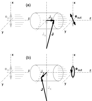
Figure 1: Schematic diagram showing the polarization response in the probe light, transmitted through the spin oriented atomic sample, on random gyrotropy (a) and random birefringence (b). Both processes are initiated by transverse fluctuations of the collective angular momentum.

V Dynamics of the system in terms of collective variables

As the most important practical example, we will further discuss the light propagation through atomic ensemble prepared originally in the coherent spin state, see figure 1. We assume that atoms fill the cylindrical volume with the cross section $S_{0}$ coinciding with the cross section of the probe light beam. The atomic ensemble is located in the homogeneous magnetic field with the direction orthogonal to the direction of the propagating light. Originally atoms are perfectly oriented along the magnetic field in the $x$ direction. Probe light is in a coherent state linearly polarized along the $x$ direction. Such a geometry is common,e.g., for experiments aiming at the quantum state teleportation between field and atomic spin subsystems DCZP ; JKP ; Polzik .

V.1 Field subsystem

Let us consider first the evolution of the Stokes components. Based on the commutation relation

$$\left[\hat{\Xi}_{i}(z^{\prime},t),\hat{\Xi}_{j}(z,t)\right]\;=\;2i\varepsilon_{ijk}\,c\,\delta(z-z^{\prime})\hat{\Xi}_{k}(z,t)$$ (32)

where $\varepsilon_{ijk}=\pm 1$ in dependence on order of indices $i\neq j\neq k$, equations (31) can be rewritten as follows

$$\left[\frac{\partial}{\partial z}+\frac{1}{c}\frac{\partial}{\partial t}\right]\hat{\Xi}_{1}(z,t) = \phantom{+}\bar{\alpha}_{1}\sum_{a=1}^{N}\hat{T}_{10}^{(a)}(t)\,\delta(z_{a}(t)-z)\,\hat{\Xi}_{3}(z,t)\;-\;\bar{\alpha}_{2}\sum_{a=1}^{N}\hat{T}_{xy}^{(a)}(t)\,\delta(z_{a}(t)-z)\,\hat{\Xi}_{2}(z,t)$$

$$\left[\frac{\partial}{\partial z}+\frac{1}{c}\frac{\partial}{\partial t}\right]\hat{\Xi}_{2}(z,t) = \phantom{+}\bar{\alpha}_{2}\sum_{a=1}^{N}\hat{T}_{xy}^{(a)}(t)\,\delta(z_{a}(t)-z)\,\hat{\Xi}_{1}(z,t)\;-\;\bar{\alpha}_{2}\sum_{a=1}^{N}\hat{T}_{\xi\eta}^{(a)}(t)\,\delta(z_{a}(t)-z)\,\hat{\Xi}_{3}(z,t)$$

$$\left[\frac{\partial}{\partial z}+\frac{1}{c}\frac{\partial}{\partial t}\right]\hat{\Xi}_{3}(z,t) = -\bar{\alpha}_{1}\sum_{a=1}^{N}\hat{T}_{10}^{(a)}(t)\,\delta(z_{a}(t)-z)\,\hat{\Xi}_{1}(z,t)\;+\;\bar{\alpha}_{2}\sum_{a=1}^{N}\hat{T}_{\xi\eta}^{(a)}(t)\,\delta(z_{a}(t)-z)\,\hat{\Xi}_{2}(z,t)$$ (33)

where we introduced the dimensionless polarizabilities

$$\bar{\alpha}_{i}\;=\;\frac{4\pi\bar{\omega}}{S_{0}\,c}\,\alpha_{i}(\bar{\omega})\ \ \ \ \ i=1,2$$ (34)

These equations are valid for any type of initial conditions and can be simplified for excitation geometry described in the preamble to this section.

The coherent forward scattering of light linearly polarized along the $x$ direction does not modify the average angular momentum orientation of the atomic ensemble. Transmitted light also preserves its mean 100% linear polarization. This means that in equations (33) only $\hat{T}_{xy}^{(a)}(t)$ and $\hat{\Xi}_{3}(z,t)$ have non-zero expectation values. Other operators exist only as fluctuating quantum variables. It is possible to linearize these equations by substituting $\hat{T}_{xy}^{(a)}(t)$ and $\hat{\Xi}_{3}(z,t)$ by their average values and leaving in the right-hand side only the linearized contribution over quantum fluctuations. Then the evolution of the Stokes operators is given by

$$\left[\frac{\partial}{\partial z}+\frac{1}{c}\frac{\partial}{\partial t}\right]\hat{\Xi}_{1}(z,t) \approx -\kappa_{2}\,\hat{\Xi}_{2}(z,t)\;+\;\bar{\alpha}_{1}\,\bar{\Xi}_{3}\,\sum_{a=1}^{N}\,\hat{T}_{10}^{(a)}(t)\,\delta(z_{a}(t)-z)\,$$

$$\left[\frac{\partial}{\partial z}+\frac{1}{c}\frac{\partial}{\partial t}\right]\hat{\Xi}_{2}(z,t) \approx \phantom{+}\kappa_{2}\,\hat{\Xi}_{1}(z,t)\;-\;\bar{\alpha}_{2}\,\bar{\Xi}_{3}\,\sum_{a=1}^{N}\,\hat{T}_{\xi\eta}^{(a)}(t)\,\delta(z_{a}(t)-z)\,$$

$$\left[\frac{\partial}{\partial z}+\frac{1}{c}\frac{\partial}{\partial t}\right]\hat{\Xi}_{3}(z,t) \approx \phantom{+}0$$ (35)

where $\bar{\Xi}_{3}=\bar{\Xi}_{0}$ is the average value of the corresponding Stokes component, which is approximately unchanged for the light beam propagating through the sample. The third line in Eqs.(35) just indicates this circumstance. The coupling parameter

$$\kappa_{2}\;=\;\bar{\alpha}_{2}\,\sum_{a=1}^{N}\,\bar{T}_{xy}^{(a)}\,\delta(z_{a}(t)-z)$$ (36)

is responsible for birefringence effects, i.e. for unitary transformation of linear polarization (defined in respect to $\xi,\;\eta$ axes) to circular polarization and vice versa. Here $\bar{T}_{xy}^{(a)}$ is the averaged and approximately unchanged value of the alignment of $a$-th atom. For any atom, whose angular momentum $j_{0}$ is oriented along the $x$ direction, the alignment term is given by

$$\bar{T}_{xy}^{(a)}\;=\;\frac{[15j_{0}(2j_{0}-1)]^{1/2}}{2[2(j_{0}+1)(2j_{0}+1)(2j_{0}+3)]^{1/2}}\;\equiv\;\bar{T}_{xy}$$ (37)

The microscopic structure of $\kappa_{2}$ can be averaged over a small mesoscopic interval of $\Delta z$ and substituted into Eq.(35) as $\kappa_{2}\,=\,\bar{\alpha}_{2}\bar{T}_{xy}n_{0}$, where $n_{0}$ is the linear density of atoms (i. e. the number of atoms per unit length). From the classical electrodynamics point of view, the mesoscopically averaged product $\kappa_{2}\lambdabar$ is the difference between refraction indices for the polarizations along $x$ and $y$ directions.

The most important terms in equations (35) are the last ones on the right hand sides. These terms show how any quantum state, originally encoded in the spin fluctuations of the atomic subsystem, can be mapped onto the polarization state of the light subsystem. Thus these terms are responsible for the quantum information processing in light - atoms interaction.

V.2 Atomic subsystem

Consider the dynamics of the orientation vector of an $a$-th atom. Applying the commutation rule for irreducible tensor operators

$$\left[\hat{T}_{KQ}^{(a)},\hat{T}_{K^{\prime}Q^{\prime}}^{(b)}\right] = \delta_{ab}\,[(2K+1)(2K^{\prime}+1)]^{1/2}\,\sum_{K^{\prime\prime}}$$ (41)

$$\times[1-(-)^{K+K^{\prime}+K^{\prime\prime}}]\,\left\{\begin{array}[]{ccc}K&K^{\prime}&K^{\prime\prime}\\ j_{0}&j_{0}&j_{0}\end{array}\right\}\,$$

$$\times\,(-)^{2j_{0}+K^{\prime\prime}}\,C^{K^{\prime\prime}Q^{\prime\prime}}_{KQ\,K^{\prime}Q^{\prime}}\,\hat{T}_{K^{\prime\prime}Q^{\prime\prime}}^{(a)}$$

see Ref.VMK , to the right hand side of equations (28) we obtain

$$\dot{\hat{T}}{}_{10}^{(a)}(t) = \frac{i}{\hbar}\left[\hat{H}_{0}(t),\,\hat{T}_{10}^{(a)}(t)\right]\;-\;\bar{\alpha}_{2}\,(-)^{2j_{0}}\sqrt{10}\,\left\{\begin{array}[]{ccc}2&1&2\\ j_{0}&j_{0}&j_{0}\end{array}\right\}\,\hat{\Xi}_{3}(z_{a}(t),t)\,\hat{T}_{\xi\eta}^{(a)}(t)$$ (47)

$$+\;\bar{\alpha}_{2}\,(-)^{2j_{0}}\sqrt{10}\,\left\{\begin{array}[]{ccc}2&1&2\\ j_{0}&j_{0}&j_{0}\end{array}\right\}\,\hat{\Xi}_{1}(z_{a}(t),t)\,\hat{T}_{xy}^{(a)}(t),$$

$$\dot{\hat{T}}{}_{1\pm 1}^{(a)}(t) = \frac{i}{\hbar}\left[\hat{H}_{0}(t),\,\hat{T}_{1\pm 1}^{(a)}(t)\right]\;\pm\;i\,\bar{\alpha}_{2}\,(-)^{2j_{0}}\frac{\sqrt{5}}{2}\,\left\{\begin{array}[]{ccc}2&1&2\\ j_{0}&j_{0}&j_{0}\end{array}\right\}\,\hat{\Xi}_{0}(z_{a}(t),t)\,\hat{T}_{2\pm 1}^{(a)}(t)$$ (57)

$$\mp\;i\,\bar{\alpha}_{2}\,(-)^{2j_{0}}\frac{\sqrt{5}}{2}\,\left\{\begin{array}[]{ccc}2&1&2\\ j_{0}&j_{0}&j_{0}\end{array}\right\}\,\hat{\Xi}_{3}(z_{a}(t),t)\,\hat{T}_{2\mp 1}^{(a)}(t)$$

$$+\;\bar{\alpha}_{2}\,(-)^{2j_{0}}\frac{\sqrt{5}}{2}\,\left\{\begin{array}[]{ccc}2&1&2\\ j_{0}&j_{0}&j_{0}\end{array}\right\}\,\hat{\Xi}_{1}(z_{a}(t),t)\,\hat{T}_{2\mp 1}^{(a)}(t)$$

$$\pm\;i\,\bar{\alpha}_{1}\,\frac{\sqrt{3}}{2[j_{0}(j_{0}+1)(2j_{0}+1)]^{1/2}}\;\hat{\Xi}_{2}(z_{a}(t),t)\,\hat{T}_{1\pm 1}^{(a)}(t)$$

As one can see these equations are not closed, since the right hand sides are expressed in terms of alignment components. Moreover the higher rank multipoles drive the dynamics of the alignment components. Thus to introduce the system of closed Heisenberg equations it is necessary to consider the coupled dynamics of all irreducible components defined for each atom.

However the dynamics of the atomic subsystem can be approximated by the dynamics of orientation components only as far as we are restricted to the discussion of the excitation regime described in the preamble to this section. As shown in the appendix B equations (57) can be transformed to the set of nonlinear equations, where the right-hand sides are expressed in terms of the operators of the angular momentum. In a special, but the most important for us, regime of small fluctuations such transformed equations can be linearized and simplified to the equations describing the dynamics of the vector of the angular momentum in a closed form. Let us define the vector of the collective angular momentum of ensemble as

$$\hat{\mathbf{J}}(t)\;=\;\sum_{a=1}^{N}\,\hat{\mathbf{j}}^{(a)}(t)$$ (58)

Then starting from equations (130), written for any $a$-th atom, and making the sum over all atoms of the ensemble, we arrive at the following equations governing the dynamics of the collective angular momentum

$$\dot{\hat{J}}_{z}(t) \approx \phantom{+}(\Omega_{0}\,+\,\Omega_{2})\,\hat{J}_{y}(t)\;-\;\bar{T}_{xy}\,\bar{\alpha}_{2}\,\sum_{a=1}^{N}\,\hat{\Xi}_{1}(z_{a}(t),t)$$

$$\dot{\hat{J}}_{y}(t) \approx -(\Omega_{0}\,+\,\Omega_{2})\,\hat{J}_{z}(t)\;+\;\frac{1}{2}\bar{T}_{x}\,\bar{\alpha}_{1}\,\sum_{a=1}^{N}\,\hat{\Xi}_{2}(z_{a}(t),t)$$

$$\dot{\hat{J}}_{x}(t) \approx \phantom{+}0$$ (59)

where parameters $\Omega_{2}$ and $\bar{T}_{x}$ are defined by expressions (131) and (132) respectively and $\bar{T}_{xy}$ is given by (37). The last source-type terms on the right hand side of these equations are responsible for the mapping of any quantum state, originally prepared in the Stokes fluctuations of the field subsystem, onto long lived atomic spin subsystem.

Equations (35) and (59), considered together, approximate the dynamical evolution of coupled collective variables of light and atomic subsystems. But as follows from the structure of these equations they are still not closed because the coupling terms are not expressed by collective variables. As we see from (35) only the atoms currently located before the wavefront contribute into formation of the fluctuating Stokes variables. In turn, such spatially dependent Stokes fluctuations, which stay actually unknown, drive the dynamics of atomic collective angular momentum via source terms in (59). However, as we show below, under certain simplifying assumptions, these equations can be further transformed into the system of closed equations describing the wave-type spatial and temporal distribution of the collective Heisenberg operators of the atomic and field subsystems.

V.3 Mesoscopic averaging

If atoms are slowly drifting in space and during the interaction with a short probe light pulse each atom preserves its location inside the area much less than the length scale comparable with $\kappa_{2}^{-1}$ or with the sample size, equations (35) and (59) can be transformed into a closed form. Let us note here that if in the experiment the duration of a probe pulse is chosen less than a few microseconds such a condition is normally fulfilled even in case of atoms at room temperature. For the case of cold trapped atoms this assumption is consistent with the pulse duration up to a second. Then the equations of motion can be rewritten for any mesoscopic layer of the sample, which gives only a small increment to the Heisenberg operators but contains a large number of atoms. The atoms do not leave the layer during the interaction time and cooperatively interact with the electromagnetic field. If this layer has a length of $\Delta z$, we can introduce the averaged Stokes operators $\hat{\Xi}_{1}(z,t)$ along this layer. As a next step, instead of total angular momentum, given by Eq.(58) we can define its mesoscopic spatial distribution as follows

$$\hat{\cal\mathbf{J}}(z,t)\;=\;\frac{1}{\Delta z}\sum_{z<z_{a}<z+\Delta z}\,\hat{\mathbf{j}}^{(a)}(t)\,$$ (60)

where the sum over $a$ is extended only over the atoms located inside the layer. Then the total angular momentum of the ensemble is expressed as

$$\hat{\mathbf{J}}(t)\;=\;\int_{0}^{L}\hat{\cal\mathbf{J}}(z,t)\,dz$$ (61)

where $dz=\Delta z$ and $L$ is the length of the sample.

The above assumptions lead us to the following set of closed and coupled equations for the mesoscopically averaged spatial distributions of the field and atomic variables

$$\left[\frac{\partial}{\partial z}+\frac{1}{c}\frac{\partial}{\partial t}\right]\hat{\Xi}_{1}(z,t) = -\kappa_{2}\,\hat{\Xi}_{2}(z,t)\;+\;2\beta\,\bar{\Xi}_{3}\,\hat{{\cal J}}_{z}(z,t)$$

$$\left[\frac{\partial}{\partial z}+\frac{1}{c}\frac{\partial}{\partial t}\right]\hat{\Xi}_{2}(z,t) = \phantom{+}\kappa_{2}\,\hat{\Xi}_{1}(z,t)\;-\;2\epsilon\,\bar{\Xi}_{3}\,\hat{{\cal J}}_{y}(z,t)$$

$$\frac{\partial}{\partial t}\hat{{\cal J}}_{z}(z,t) = \phantom{+}\Omega\,\hat{{\cal J}}_{y}(z,t)\;-\;\theta_{y}\bar{{\cal J}}_{x}\,\hat{\Xi}_{1}(z,t)$$

$$\frac{\partial}{\partial t}\hat{{\cal J}}_{y}(z,t) = -\Omega\,\hat{{\cal J}}_{z}(z,t)\;+\;\theta_{z}\bar{{\cal J}}_{x}\,\hat{\Xi}_{2}(z,t)$$

where we used the same notation for the averaged Stokes variables as for their microscopic origins and denoted the mesoscopic spatial distributions of angular momentum components as $\hat{\cal J}_{\mu}(z,t)$, with $\mu=x,y,z$. It is taken into account that $\bar{{\cal J}}_{x}(z,t)=\bar{{\cal J}}_{x}=const$. Equations (LABEL:5.12) should be accompanied by corresponding initial and boundary conditions, which are given by

$$\hat{\Xi}_{1}(0,t) = \hat{\Xi}_{1}^{in}(t)$$

$$\hat{\Xi}_{2}(0,t) = \hat{\Xi}_{2}^{in}(t)$$

$$\hat{{\cal J}}_{y}(z,0) = \hat{{\cal J}}_{y}^{in}(z)$$

$$\hat{{\cal J}}_{z}(z,0) = \hat{{\cal J}}_{z}^{in}(z)$$ (63)

The solution of these equations presented in the next section shows how the swapping of quantum fluctuations between light and spin subsystems takes place during the interaction process.

Several new parameters appear in equations (LABEL:5.12). Firstly, by $\Omega$ we denote the frequency $\Omega=\Omega_{0}+\Omega_{2}$ of the regular precession caused by the external magnetic field as well as by the light-induced shift of the Zeeman sublevels. Secondly, there are two new parameters in the first pair of equations describing the transformation of the Stokes variables. The angle $\beta$

$$\beta\;=\;\frac{\sqrt{3}}{2[j_{0}(j_{0}+1)(2j_{0}+1)]^{1/2}}\,\bar{\alpha}_{1}$$ (64)

is the angle of Faraday-type rotation of the polarization plane of the propagating light per one spin flip in the ensemble in $z$-direction. The parameter $\epsilon$

$$\epsilon\;=\;\frac{[15(2j_{0}-1)]^{1/2}}{2[2j_{0}(j_{0}+1)(2j_{0}+1)(2j_{0}+3)]^{1/2}}\,\bar{\alpha}_{2}$$ (65)

is the ellipticity induced in the propagating light by the atomic sample per one spin flip in $y$-direction, see figure 1. Thirdly, there are two angles in the second pair of equations describing the dynamics of the spatial distribution of the atomic angular momenta. Angle $\theta_{y}=\epsilon$ is the rotation angle of the local collective angular momentum, originally oriented along $x$-axis, around $y$-axis per one photon propagating trough the sample in either $\xi$-type or $\eta$-type linear polarization. In turn, angle $\theta_{z}=\beta$ is the rotation angle of the local angular momentum around $z$-axis per one photon propagating through the sample in either right-hand-type or left-hand-type circular polarization.

VI Entanglement of the quantum states of light and atoms

For pedagogical purposes, we consider at first a special example of optical excitation in the far-off-resonance wing of $j_{0}=1/2\to j=1/2$ or $j_{0}=1/2\to j=3/2$ optical transitions and will discuss the general case after that.

VI.1 Example of $j_{0}=1/2\to j=1/2,\,j=3/2$ optical transitions

In the case of $j_{0}=1/2\to j=1/2$ or $j_{0}=1/2\to j=3/2$ transition equations (LABEL:5.12) are simplified to the following form

$$\left[\frac{\partial}{\partial z}\,+\,\frac{1}{c}\frac{\partial}{\partial t}\right]\hat{\Xi}_{1}(z,t) = \phantom{+}2\beta\,\bar{\Xi}_{3}\,\hat{{\cal J}}_{z}(z,t)$$

$$\left[\frac{\partial}{\partial z}\,+\,\frac{1}{c}\frac{\partial}{\partial t}\right]\hat{\Xi}_{2}(z,t) = \phantom{+}0$$

$$\frac{\partial}{\partial t}\hat{{\cal J}}_{z}(z,t) = \phantom{+}\Omega_{0}\,\hat{{\cal J}}_{y}(z,t)$$

$$\frac{\partial}{\partial t}\hat{{\cal J}}_{y}(z,t) = -\Omega_{0}\,\hat{{\cal J}}_{z}(z,t)\;+\;\beta\bar{{\cal J}}_{x}\,\hat{\Xi}_{2}(z,t)$$

where it was taken into account that $\bar{\alpha}_{2}=0$ and therefore $\kappa_{2}=0$, $\Omega_{2}=0$, $\epsilon=\theta_{y}=0$. Because of the second line in the system (LABEL:6.1), one has $\hat{\Xi}_{2}(z,t)=\hat{\Xi}_{2}^{in}(t-z/c)$.

The straightforward solution for the distribution of the angular momentum components leads to

$$\hat{{\cal J}}_{z}(z,t) = \phantom{+}\cos\Omega_{0}t\;\hat{{\cal J}}_{z}^{in}(z)\,+\,\sin\Omega_{0}t\;\hat{{\cal J}}_{y}^{in}(z)\;+\;\beta\bar{{\cal J}}_{x}\,\int_{0}^{t}dt^{\prime}\sin\Omega_{0}(t-t^{\prime})\;\hat{\Xi}_{2}^{in}(t^{\prime}-z/c)$$

$$\hat{{\cal J}}_{y}(z,t) = -\sin\Omega_{0}t\;\hat{{\cal J}}_{z}^{in}(z)\,+\,\cos\Omega_{0}t\;\hat{{\cal J}}_{y}^{in}(z)\,+\,\beta\bar{{\cal J}}_{x}\;\int_{0}^{t}dt^{\prime}\cos\Omega_{0}(t-t^{\prime})\;\hat{\Xi}_{2}^{in}(t^{\prime}-z/c)$$ (67)

and the Stokes component $\hat{\Xi}_{1}(z,t)$ is given by

$$\hat{\Xi}_{1}(z,t) = \hat{\Xi}_{1}^{in}(t-z/c)\,+\,2\beta\,\bar{\Xi}_{3}\,\int_{0}^{z}\!dz^{\prime}\,\hat{{\cal J}}_{z}(z^{\prime},t-(z-z^{\prime})/c)\;=\;\hat{\Xi}_{1}^{in}(t-z/c)$$ (68)

$$+\;2\beta\,\bar{\Xi}_{3}\,\int_{0}^{z}\!dz^{\prime}\,\cos\Omega_{0}[t-(z-z^{\prime})/c]\;\hat{{\cal J}}_{z}^{in}(z^{\prime})\;+\;2\beta\,\bar{\Xi}_{3}\,\int_{0}^{z}\!dz^{\prime}\,\sin\Omega_{0}[t-(z-z^{\prime})/c]\;\hat{{\cal J}}_{y}^{in}(z^{\prime})$$

$$+\;2\beta^{2}\,\bar{\Xi}_{3}\bar{{\cal J}}_{x}\int_{0}^{z}\!dz^{\prime}\!\int_{0}^{t-(z-z^{\prime})/c}\!dt^{\prime}\sin\Omega_{0}[t-t^{\prime}-(z-z^{\prime})/c]\;\hat{\Xi}_{2}^{in}(t^{\prime}-z^{\prime}/c)$$

This solution explains the basic idea of entanglement of the collective quantum states of atomic and field subsystems. After the interaction cycle the quantum state of light described by the $\hat{\Xi}_{2}^{in}$ component is mapped onto the atomic angular momentum components because of the last terms in Eqs.(67). In turn, the information written in either $\hat{{\cal J}}_{z}^{in}$ or $\hat{{\cal J}}_{y}^{in}$ components of the angular momentum is mapped onto the $\hat{\Xi}_{1}$ Stokes component of light, because of the second and third terms in Eq.(68). Moreover, due to atom-field interaction there is a partial mapping of the $\hat{\Xi}_{2}^{in}$ component onto $\hat{\Xi}_{1}$ component because of the last term in Eq.(68).

The retardation effects, which are clearly visible in the derived solution are mainly important in order to preserve the proper commutation relations for the whole set of the Heisenberg operators involved in the process. The initial zero moment of time is a conventional and arbitrary chosen parameter to coordinate Schrödinger and Heisenberg pictures. Physically the interaction cycle starts only when the wavefront of the probe radiation crosses $z=0$ point. We will take this time as the initial moment $t=0$. In the Heisenberg formalism this means that any expectations values of $\hat{\Xi}_{1}^{in}(t)$ and $\hat{\Xi}_{2}^{in}(t)$ operators or their products are equal to zero for time $t<0$. Since the goal is to evaluate the expectation values of outgoing operators it is acceptable to substitute the lower zero limit by $t\to z/c$ in (67) and by $t^{\prime}\to z^{\prime}/c$ in the internal integral (68). Then the derived solution can be further applied at any spatial point $z$ only for time $t>z/c$, which is in accordance with physical manifestation of retardation effects.

In reality, we are most interested in a correct description of the behavior of the modes around the carrier frequency $\bar{\omega}$, see definition (29). For the modes distributed in the spectral domain much narrower than $c/L$, where $L$ is the length of the sample, the retardation effects become negligible. In this case the above solution is simplified and can be written in terms of transverse components of the collective angular momentum

$$\hat{J}_{z}(t) = \phantom{+}\cos\Omega_{0}t\;\hat{J}_{z}^{in}\,+\,\sin\Omega_{0}t\;\hat{J}_{y}^{in}\;+\;\beta\bar{J}_{x}\,\int_{0}^{t}dt^{\prime}\sin\Omega_{0}(t-t^{\prime})\;\hat{\Xi}_{2}^{in}(t^{\prime})$$

$$\hat{J}_{y}(t) = -\sin\Omega_{0}t\;\hat{J}_{z}^{in}\,+\,\cos\Omega_{0}t\;\hat{J}_{y}^{in}\,+\,\beta\bar{J}_{x}\;\int_{0}^{t}dt^{\prime}\cos\Omega_{0}(t-t^{\prime})\;\hat{\Xi}_{2}^{in}(t^{\prime})$$ (69)

and for the output Stokes operator $\hat{\Xi}_{1}^{out}(t)$

$$\hat{\Xi}_{1}^{out}(t) = \hat{\Xi}_{1}^{in}(t)\phantom{+\;2\beta\,\bar{\Xi}_{3}\cos\Omega_{0}t\,\hat{J}_{z}^{in}\;+\;2\beta\,\bar{\Xi}_{3}\sin\Omega_{0}t\,\hat{J}_{y}^{in}}$$ (70)

$$+\;2\beta\,\bar{\Xi}_{3}\cos\Omega_{0}t\,\hat{J}_{z}^{in}\;+\;2\beta\,\bar{\Xi}_{3}\sin\Omega_{0}t\,\hat{J}_{y}^{in}$$

$$+\;2\beta^{2}\,\bar{\Xi}_{3}\bar{J}_{x}\,\int_{0}^{t}dt^{\prime}\sin\Omega_{0}(t-t^{\prime})\;\hat{\Xi}_{2}^{in}(t^{\prime})$$

which coincides, in principle, with the solution obtained earlier in Refs.JKP ; H .

The input-output transformations expressed by (69) and (70) have a simple logical structure and therefore are attractive for possible applications to the quantum information tasks. However, they are only valid for $j_{0}=1/2\to j=1/2,j=3/2$ isolated transitions, and it is rather difficult to find a practical example of such a transition. However, the same simple input-output relations are effectively realized in the case of alkali atoms excited in the far wing of $D_{1}$ or $D_{2}$ lines. In this case the contributions from the components of the upper hyperfine multiplet to the interaction add up in such a way that the alignment effects become unimportant. For a transition from the ground hyperfine state $F_{0}$ to all hyperfine states $F$ we straightforwardly obtain after taking the sum over the excited states

$$\sum_{F}\,\bar{\alpha}_{2} \propto \sum_{F}\,\frac{|d_{j_{0}j}|^{2}}{-\hbar\Delta_{F}}\,(-)^{F+F_{0}+1}\,(2F+1)(2F_{0}+1)\,$$ (75)

$$\times\left\{\begin{array}[]{ccc}1&1&2\\ F_{0}&F_{0}&F\end{array}\right\}\,\left\{\begin{array}[]{ccc}I&j&F\\ 1&F_{0}&j_{0}\end{array}\right\}^{2}\;\to\;0$$

Hence the alignment contribution vanishes for the ground state electronic angular momentum $j_{0}=1/2$ if the frequency detuning $\Delta_{F}=\bar{\omega}-\omega_{FF_{0}}$ for each hyperfine transition $F_{0}\to F$ becomes larger than the hyperfine splitting of the upper state. The crucial inequality $|\bar{\alpha}_{1}|\gg|\bar{\alpha}_{2}|$ which allows to neglect the alignment effects is fulfilled the better the less important is the dependence on the upper hyperfine momentum in the denominator of (75). In spite of the fact that for heavy alkali atoms the ratio of the hyperfine to fine splitting in the upper state $\delta E_{hf}/\delta E_{f}$ is really small (it is less than $10^{-4}$ for ¹³³Cs), which makes it possible to neglect the alignment contribution for large detunings, such an approximation is not always easy to fulfill under typical experimental conditions. This is because for a large frequency detuning one has to use pulses with a very large photon number in order to make the atom-field interaction strong enough. Large photon numbers are often inconvenient due to either limitations of detectors or due to a limited pulse duration, or both. Therefore the frequency detuning $\Delta$ is frequently chosen to be comparable with $\delta E_{hf}$. A typical detuning chosen in the experiment JKP , is of the order of $900\;MHz$ with the hyperfine splitting in $6{}^{2}P_{3/2}$ of $\delta E_{hf}\sim 200\;MHz$. This is one of the motivations for the deeper analysis of equations (LABEL:5.12) in their general form.

VI.2 General solution

Equations (LABEL:5.12) can be solved in the general case, which we do first ignoring the retardation effects. This is the most important case for practical applications to quantum information processing. Without retardation the system of coupled equations (LABEL:5.12) can be rewritten as follows

$$\frac{\partial}{\partial z}\hat{\Xi}_{1}(z,t) = -\kappa_{2}\,\hat{\Xi}_{2}(z,t)\;+\;2\beta\,\bar{\Xi}_{3}\,\hat{{\cal J}}_{z}(z,t)$$

$$\frac{\partial}{\partial z}\hat{\Xi}_{2}(z,t) = \phantom{+}\kappa_{2}\,\hat{\Xi}_{1}(z,t)\;-\;2\epsilon\,\bar{\Xi}_{3}\,\hat{{\cal J}}_{y}(z,t)$$

$$\frac{\partial}{\partial t}\hat{{\cal J}}_{z}(z,t) = \phantom{+}\Omega\,\hat{{\cal J}}_{y}(z,t)\;-\;\theta_{y}\bar{{\cal J}}_{x}\,\hat{\Xi}_{1}(z,t)$$

$$\frac{\partial}{\partial t}\hat{{\cal J}}_{y}(z,t) = -\Omega\,\hat{{\cal J}}_{z}(z,t)\;+\;\theta_{z}\bar{{\cal J}}_{x}\,\hat{\Xi}_{2}(z,t)$$ (76)

This is a set of differential equations with constant coefficients and it is accompanied by initial and boundary conditions (63). The solution can be presented in the form of an integral response on these conditions. For the Stokes operators it can be written as

$$\hat{\Xi}_{i}(z,t) = \sum_{j=1,2}\,\int_{0}^{t}dt^{\prime}\,{\cal M}_{ij}(z,t-t^{\prime})\,\hat{\Xi}_{j}^{in}(t^{\prime})\phantom{{\cal F}_{i\nu}(z-z^{\prime},t)\,}$$ (77)

$$+\;\sum_{\nu=z,y}\,\int_{0}^{z}dz^{\prime}\,{\cal F}_{i\nu}(z-z^{\prime},t)\,\hat{{\cal J}}_{\nu}^{in}(z^{\prime})$$

with $i=1,2$. For the operators of the spatial distributions of the angular momentum components the solution is

$$\hat{{\cal J}}_{\mu}(z,t) = \sum_{j=1,2}\,\int_{0}^{t}dt^{\prime}\,{\cal G}_{\mu j}(z,t-t^{\prime})\,\hat{\Xi}_{j}^{in}(t^{\prime})\phantom{{\cal N}_{\mu\nu}(z-z^{\prime},t)\,}$$ (78)

$$+\;\sum_{\nu=z,y}\,\int_{0}^{z}dz^{\prime}\,{\cal N}_{\mu\nu}(z-z^{\prime},t)\,\hat{{\cal J}}_{\nu}^{in}(z^{\prime})$$

with $\mu=z,y$. The solution can be formally extended over the space-time region $0<t<\infty$ and $0<z<\infty$.

As shown in the appendix C, the kernels of the integral transformations in (77) and (78) can be expressed via the corresponding Laplace images

$${\cal K}(z,t)\;=\;\frac{1}{(2\pi i)^{2}}\int_{p_{0}-i\infty}^{p_{0}+i\infty}\int_{s_{0}-i\infty}^{s_{0}+i\infty}{\cal K}(p,s)\,e^{pz+st}\,dp\,ds$$ (79)

where ${\cal K}(z,t)$ is any of the matrix functions ${\cal M}(z,t),\ldots,{\cal N}(z,t)$ in equations (77) and (78) and ${\cal K}(p,s)$ is its Laplace image. The limits of integration $p_{0}$ and $s_{0}$ are chosen as arbitrary real values warranting the existence of Laplace images for the spatial and temporal transforms respectively. In the appendix C the images for all the matrices ${\cal M}(p,s),\ldots,{\cal N}(p,s)$ are calculated explicitly. Evaluation of the integrals (79) can be done numerically for any sample when all the external parameters are defined.

Let us briefly explain how the retardation effects can be taken into account. To do this the retardation time $\tau=t-z/c$ should be introduced as an independent variable for each spatial point $z$ at a certain moment of time $t$. Then the basic system (LABEL:5.12), where all the operators are considered now as functions of $z$ and $\tau$, can be converted to the form (76) but with the derivative over retardation time on the left hand side. The initial conditions should be also modified and written for the initial retardation time $\tau=0$, which corresponds now to spatially dependent moments in the laboratory time $t=z/c$. As before we will assume that the wavefront of the probe radiation crosses $z=0$ point at zero time. In this case we need to know the cooperative atom-field dynamics at any spatial point $z$ only for time $t>z/c$. Then we may ignore the interaction Hamiltonian for time $0<t<z/c$ and chose the initial conditions in (63) in the following form

$$\hat{{\cal J}}_{z}(z,\tau=0) = \phantom{+}\cos(\Omega_{0}z/c)\;\hat{{\cal J}}_{z}^{in}(z)\phantom{\sin(\Omega_{0}z/c)\;\hat{{\cal J}}_{y}^{in}(z)}$$

$$+\,\sin(\Omega_{0}z/c)\;\hat{{\cal J}}_{y}^{in}(z)\;\equiv\;\hat{{\cal J}}_{z}^{in\prime}(z)$$

$$\hat{{\cal J}}_{y}(z,\tau=0) = -\sin(\Omega_{0}z/c)\;\hat{{\cal J}}_{z}^{in}(z)$$ (80)

$$+\,\cos(\Omega_{0}z/c)\;\hat{{\cal J}}_{y}^{in}(z)\;\equiv\;\hat{{\cal J}}_{y}^{in\prime}(z)$$

There are no changes in the boundary conditions in (63), since at $z=0$ the retardation time $\tau$ coincides with $t$. Thus in the most general case the solution (77)-(79) should be rewritten in terms of the retardation time and should depend on $\hat{{\cal J}}_{z}^{in\prime}(z)$ and $\hat{{\cal J}}_{y}^{in\prime}(z)$ as on initial quantum fluctuations of the atomic angular momenta.

Finally the retardation effects give us the following correction to the spatial and temporal dynamics of the field variables

$$\hat{\Xi}_{i}(z,t)\;=\;\sum_{j=1,2}\,\int_{0}^{t-z/c}dt^{\prime}\,{\cal M}_{ij}(z,t-z/c-t^{\prime})\,\hat{\Xi}_{j}^{in}(t^{\prime})\;+\;\sum_{\nu=z,y}\,\int_{0}^{z}dz^{\prime}\,{\cal F}_{i\nu}(z-z^{\prime},t-z/c)\,\hat{{\cal J}}_{\nu}^{in\prime}(z^{\prime})$$ (81)

and of the atomic variables

$$\hat{{\cal J}}_{\mu}(z,t)\;=\;\sum_{j=1,2}\,\int_{0}^{t-z/c}dt^{\prime}\,{\cal G}_{\mu j}(z,t-z/c-t^{\prime})\,\hat{\Xi}_{j}^{in}(t^{\prime})\;+\;\sum_{\nu=z,y}\,\int_{0}^{z}dz^{\prime}\,{\cal N}_{\mu\nu}(z-z^{\prime},t-z/c)\,\hat{{\cal J}}_{\nu}^{in\prime}(z^{\prime})$$ (82)

These expressions can be applied for calculation of expectation values of any products of operators at a spatial point $z$ for the time $t>z/c$.

An important feature of solutions (81) and (82) is their wave nature. As follows from the Laplace transform carried out in the Appendix C the eigenmodes of spatial and temporal distributions of atoms-field collective fluctuations are associated with the poles of determinant $\Delta(p,s)\to 0$, where $\Delta(p,s)$ is defined by (135). For atoms with spin $1/2$ this condition leads to $p\to 0$ and $s\to\pm{\rm i}\Omega_{0}$. In the absence of the magnetic field $\Omega_{0}\to 0$ there are only two collective modes associated with the total number of atoms and with the total number of scattering photons which undergo polarization sensitive interaction in the process of coherent forward scattering. This makes it possible to further simplify the effective Hamiltonian and to discuss it in terms of integrated collective variables of the canonical type KzPl ; JKP .

However in a general case, due to presence of alignment associated effects, the condition $\Delta(p,s)\to 0$ gives coupled roots $s=s(p)$, i.e the wave-type modes which can survive in the sample and be excited by either time dependent fluctuations of the field Stokes components or by spatial fluctuations of atomic spins. Such quantum superposition of the field and material waves can be understood as a polariton-type spin wave generated in the medium. The multimode structure of such waves does not allow entanglement only between integrated collective variables. Instead, in general the entanglement is distributed in all polariton modes. From the quantum information point of view this means that in the case of atoms with the ground state angular momentum equal or larger than $1$ a possible entanglement resource hidden in the polariton modes allows for multimode entanglement rather than a single mode entanglement available for spin one half systems. The quantum information then will be mapped on spatially dependent correlations of an atomic standing spin wave.

The following remark concerning the terminology is due here. Let us point out the principle difference between the spin-wave dynamics described by Eqs.(5.13) and the collective spin behavior in the spin-organized cold fermion gas, which was discussed years ago, see BLL . In our case the cooperative dynamics of atomic spins is driven by the radiation-type interaction whereas in the cold fermionic systems it is driven by the static interparticle interaction via the longitudinal electric field.

VI.3 Spin squeezing in an ensemble of cesium atoms.

In this section we concentrate on calculations relevant for the existing experimental example JKP carried out with ensemble(s) of ¹³³Cs atoms. We first calculate the degree of spin squeezing ignoring the alignment, i.e., following the model adopted in JKP and describing the atomic ground state by the spin (orientation) only. We then present the numerical results including the alignment and show how this affects spin squeezing of atoms.

In the experiment JKP the entanglement (two mode squeezing) was generated between two spatially separated via a Faraday-type detection of light. For pedagogical reasons we will make numerical simulations for the case of single mode spin squeezing, which makes no difference for the present discussion. We will completely ignore the retardation effects and consider the spin dynamics without external magnetic field.

In the case of cesium atoms the alignment contribution can be suppressed if the frequency detuning of the probe light from the atomic resonance is much larger than the hyperfine splitting in the upper state, as described in the end of section VI.1. If the alignment is ignored the basic equations stem from the expressions (69) and (70), which in the absence of magnetic field read

$$\hat{J}_{z}(t) = \phantom{+}\hat{J}_{z}^{in}$$

$$\hat{J}_{y}(t) = \hat{J}_{y}^{in}\,+\,\beta\bar{J}_{x}\;\int_{0}^{t}dt^{\prime}\hat{\Xi}_{2}^{in}(t^{\prime})$$

$$\hat{\Xi}_{1}^{out}(t) = \hat{\Xi}_{1}^{in}(t)\;+\;2\beta\,\bar{\Xi}_{3}\,\hat{J}_{z}^{in}$$

$$\hat{\Xi}_{2}^{out}(t) = \hat{\Xi}_{2}^{in}(t)$$ (83)

The input-output transformations (83) show the entangling mechanism of the atoms-field variables in the process of coherent forward scattering. If the number of atoms and photons is large enough such as $\beta\bar{J}_{x}\gg 1$ and $\beta\bar{\Xi}_{3}t\gg 1$ the output quantum fluctuations become strongly entangled. Indeed, in this case the role of $\hat{J}_{y}^{in}$ and $\hat{\Xi}_{1}^{in}(t)$ terms on the right hand side of (83) becomes negligible if these fluctuations have been originally Poissonian. After the interaction there would be strong correlations between fluctuations of $\int_{0}^{t}\hat{\Xi}_{1}^{out}(t^{\prime})dt^{\prime}$ and $\hat{J}_{z}(t)$ as well as between $\hat{J}_{y}(t)$ and $\int_{0}^{t}\hat{\Xi}_{2}^{out}(t^{\prime})dt^{\prime}$. If the observable $\int_{0}^{t}\hat{\Xi}_{1}^{out}(t^{\prime})dt^{\prime}$ is measured by a balanced Faraday detector there will be no longer standard quantum uncertainty in $\hat{J}_{z}(t+0)$, whose original (at $t\to 0$) Poissonian fluctuations will be suppressed by a factor $\beta\bar{\Xi}_{3}t\gg 1$. The collective spin state will become squeezed and will accumulate its quantum uncertainty in $\hat{J}_{y}(t+0)$ fluctuation.

It is important to recognize that even in such an ideal scheme there is a restriction on the number of participating atoms and photons because of accumulation of events of the incoherent scattering. It is clear that in each event of the incoherent scattering one photon and one atom of the ensemble cancel out from entangling process. These losses can be neglected if the number of scattering events is much less than the total numbers of atoms $N_{a}$ and incoming photons $N_{ph}$. This can be written as two inequalities

$$\frac{\sigma_{\Delta}}{S_{0}}\,N_{ph}N_{a} \ll N_{a}$$

$$\frac{\sigma_{\Delta}}{S_{0}}\,N_{ph}N_{a} \ll N_{ph}$$ (84)

where $\sigma_{\Delta}$ is the cross section for off-resonant incoherent scattering in full solid angle, and $S_{0}$ is the area of the light beam, which coincides with the area of atomic cloud. Both inequalities lead to similar restrictions on the number of participating atoms and photons

$$N_{a},N_{ph}\;\ll\;\frac{S_{0}}{\sigma_{\Delta}}$$ (85)

In case of photons this inequality can be also understood as a restriction on the whole interaction time $T$ (the probe pulse duration), since $N_{ph}=\bar{\Xi}_{0}T=\bar{\Xi}_{3}T$. Since both type of the losses are undesirable one can assume that $N_{a}=N_{ph}$ to exclude any preference for atoms or photons. The number of scattered photons can be expressed as

$$N_{ph}\;=\;\eta\frac{S_{0}}{\sigma_{\Delta}}$$ (86)

where by small parameter $\eta$ we denoted the relative number of atoms and photons lost as a result of incoherent scattering, see the first line of (84). A detailed analysis of the role of spontaneous emission is presented in Polzik .

The scheme of energy levels of ¹³³Cs is shown in figure 2. Skipping technical details of calculation of off-resonant cross section $\sigma_{\Delta}$ (on an atom in the Zeeman sublevel $F_{0}=4,M_{0}=4$ of its ground state) and of estimation of the elementary Faraday angle $\beta$, we present the final result. The square variance of any output Stokes component $\Xi_{i}^{out}$, where $i=1,2$, is given by

$$\left\langle\left[\int_{0}^{T}\hat{\Xi}_{i}^{out}(t)dt\right]^{2}\right\rangle\;=\;\bar{\Xi}_{3}T\,\left[1\,+\,\xi_{i}(J)\right]$$ (87)

where the Mandel parameter $\xi_{i}(J)$, considered as function of the total collective angular momentum $J\approx\bar{J}_{x}$, shows the relative deviation from the shot-noise level. This deviation is due to the variance of the atomic state mapped onto the output light. For $\hat{\Xi}_{1}^{out}$ Stokes component the original value of the Mandel parameter $\xi_{1}$ transforms as

$$\xi_{1}(J) = \xi_{1}\,+\,2\eta\,f\left(\frac{\gamma}{\Delta_{5}},\frac{\gamma}{\Delta_{4}},\frac{\gamma}{\Delta_{3}}\right)\,\beta J$$ (88)

$$\equiv \xi_{1}\,+\,\kappa^{2}$$

where the second line defines the dimensionless parameter $\kappa$ responsible for coupling of the field and atomic subsystems described in terms of their canonical variable, see Polzik . For $\hat{\Xi}_{2}^{out}$ component the Mandel parameter preserves its magnitude, so that $\xi_{2}(J)=\xi_{2}$. In (88) and throughout we approximate the input fluctuations as Markovian delta-correlated process in the lower frequency domain

$$\left\langle\hat{\Xi}_{i}^{in}(t^{\prime})\hat{\Xi}_{i}^{in}(t)\right\rangle\;=\;\bar{\Xi}_{3}\,(1+\xi_{i})\,\delta(t^{\prime}-t)$$ (89)

and assume the Poissonian (coherent state) square variance of the angular momentum $\langle J_{z}^{2}\rangle=\bar{J}_{x}/2=J/2$ for original coherent atomic spin state. Second term in (88) denotes the contribution of the Faraday effect itself and function $f(\ldots)$ denotes the product

$$\beta\,\frac{S_{0}}{\sigma_{\Delta}} \equiv f\left(\frac{\gamma}{\Delta_{5}},\frac{\gamma}{\Delta_{4}},\frac{\gamma}{\Delta_{3}}\right)$$ (90)

$$= \frac{\frac{11}{60}\frac{\gamma}{\Delta_{5}}-\frac{7}{320}\frac{\gamma}{\Delta_{4}}-\frac{7}{192}\frac{\gamma}{\Delta_{3}}}{\frac{3}{10}\frac{\gamma^{2}}{\Delta_{5}^{2}}+\frac{7}{10}\frac{\gamma^{2}}{\Delta_{4}^{2}}}$$

where $\gamma$ is the rate of the spontaneous decay of the upper state and $\Delta_{j}=\omega-\omega_{j4}$ with $j=3,4,5$ are the frequency detunings of the probe light from each exciting hyperfine transition, see figure 2.

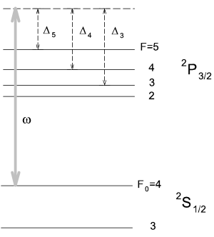
Figure 2: Energy level diagram of $D_{2}$-line of ¹³³Cs: $\Delta_{5}$, $\Delta_{4}$, and $\Delta_{3}$ are the frequency detunings of the probe light from hyperfine transitions participating in the process.

Note that, as a consequence of neglecting the alignment effects, the total angular momentum (or a number of atoms) contributes in the output Mandel parameter only in combination $\beta J$. This parameter is the optical activity of the sample, i.e. the angle of Faraday rotation of the planar wave for the ensemble perfectly oriented along the probe beam, see figure 1. This linearity (see dashed-dotted lines in figures 3-5) has been used as the benchmark for the determination of the projection noise level of atoms in all the work related to quantum state generation with atomic ensembles, see for example Polzik .

As follows from the above discussion of the role of spontaneous emission, a reasonable choice of parameters for spin squeezing corresponds to $\beta J\sim F_{0}\eta f(\ldots)=4\eta f(\ldots)$. Under typical conditions for the frequency detuning $\Delta_{5}\sim 1000\,MHz$ and $\eta\sim 0.1$ the optical activity can be $\beta J\sim 1$, which can provide spin squeezing far below the standard quantum limit in (87).

In order to calculate the corrections to the variances of the output Stokes components for a realistic alkali atom at a finite detuning the alignment associated effects have to be included in calculations. This can be done only numerically by means of the transformations (77). In figures 3-5 we plot the results of these calculations. The variances of the Stokes components $\hat{\Xi}_{1}^{out}$ and $\hat{\Xi}_{2}^{out}$ are shown as a function of the optical activity of the sample $\beta J$, calculated for different frequency offsets $\Delta_{5}=700,\,1000,\,1200\,MHz$ and for $\eta=0.1$. In the figures the solid curves represent the complete result within the described model, whereas dashed curves are computed only including the partial contribution coming from the first term in Eq.(77). These curves show the excessive atomic spin fluctuations, mapped onto the Stokes collective variable of the transmitted light, beyond the level of the transformed original light fluctuations and beyond the level of the spin (orientation) projection noise. The incoming light is taken to be in a coherent state with Poissonian statistics and with $\xi_{1}=\xi_{2}=0$. The enhancement of the light noise is caused by higher orders of the interaction process. Considered at certain value of $\beta J$ the difference between the complete variance and the background level shows the efficiency of the Faraday detector as a spin squeezer. The scheme works the better the higher this difference is. However, because of the alignment the squeezing has to be considered not for a collective angular momentum but for a more complex type of a spatial spin mode, which is defined by the input-output transformations (77) and (78). Squeezing and entanglement for such spatial modes will be considered elsewhere.

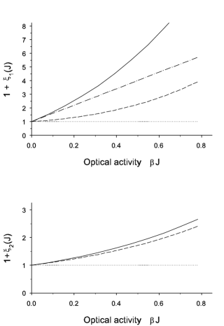
Figure 3: The Mandel parameters for the output square variances of the Stokes components $\Xi_{1}^{out}$ (upper plot) and $\Xi_{2}^{out}$ (lower plot) as a function of optical activity of the sample for the frequency offset $\Delta_{5}=700\,MHz$. The dotted curve indicates the original shot-noise level, the dashed curve is the atomic signal coming from the first term in (77), the dashed-dotted linear dependence is the Faraday approximation (88), the solid curve is the complete output variance.

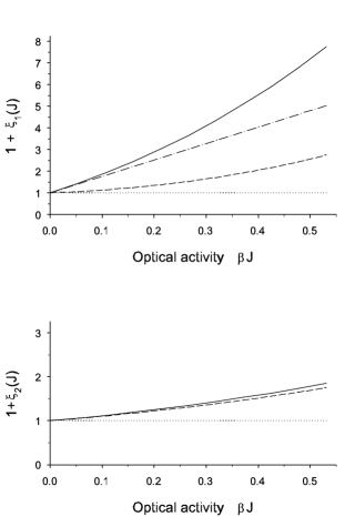
Figure 4: Same as in figure 3 for the frequency offset $\Delta_{5}=1000\,MHz$.

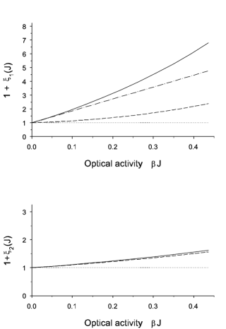
Figure 5: Same as in figure 3 for the frequency offset $\Delta_{5}=1200\,MHz$.

It is instructive to compare the result of numerical calculations with the approximation ignoring the alignment effects. The dashed-dotted linear dependencies in figures 3-5 reproduces the ideal result described by Eq.(88). As we see, for small values of $\beta J$ the Faraday approximation fits the exact solution with rather good accuracy and the deviation of $\xi_{2}$ from zero is quite small. This means that for the sample characterized by rather small optical activity the spin one-half approximation for the multi-level cesium atom is self-consistent and potentially good for describing the real experimental situation. Hence for such a sample the squeezed spin standing wave can be approximated by the collective angular momentum. Let us point out here that in the existing experiment JKP the optical activity was $\beta J<0.2$ and the alignment correction was not so important. However, as clearly seen for large $\beta J$ the difference between the input-output transformations in their general form and approximation (83) becomes quite important.

VII Conclusion

We have considered the quantum theory of coherent forward scattering of light by an ensemble of multi-level atoms polarized in their angular momenta. As a result of such a scattering process the quantum states of the field and atomic subsystems are transformed into an entangled state. In our discussion of the process we followed the effective Hamiltonian approach, which in the semiclassical form is normally applied for studying optical pumping processes after adiabatic elimination of the excited state. Compared to earlier studies of entanglement of light and atomic ensembles, we have derived the effective Hamiltonian in a more general form for the atoms with an arbitrary total magnetic momentum. Towards this end, we have found the physical conditions under which the analysis can be simplified by introducing a finite number of collective variables for light and atoms.

We showed that under certain conditions the cooperative atoms-field dynamics can be properly described by the wave-type coupled equations for the space-time evolution of the collective Heisenberg operators of the field and atomic subsystems. In these equations an infinite set of atom-field operators is truncated via introduction of slowly varying collective modes. The coupled equations for the time evolution of spatially dependent operators of the Stokes components of light and of the macroscopic fluctuations of the collective atomic angular momentum are written in a closed form. In the general case the coupled dynamics of the atom and field operators manifests itself in a spin polariton wave created in the sample. The fluctuating components of atoms and field become strongly entangled in the polariton wave in space and time. Such spin polariton waves initiated by radiative forces are different from the collective spin dynamics existing in the spin-polarized quantum gas BLL . They are also different from the polariton modes discussed in Lukin where polaritons of the combined atom-light state are introduced. In our case the quantum entanglement arises from the interaction between the internal collective polarization degrees of freedom of light and atomic subsystems. In particular our analysis yields the input-output transformations for the Heisenberg operators of the collective variables of light and atomic spins after the whole interaction cycle. Our results suggest that a successful approach of using off-resonant light-atomic ensemble interaction for quantum information processing can become even more fruitful with the use of a multi-mode type of entanglement provided by spin polariton atomic variables.

Numerical simulations demonstrate the importance of the developed formalism for application to a realistic experimental situation. We considered a well known example, when the Faraday rotation is used as a non-demolishing measurement of transverse fluctuations of the collective atomic spin and can be utilized as a physical mechanism for the spin squeezing in an ensemble of spin polarized atoms. We tested the validity of the spin one-half approximation for a realistic Cesium atom, which is normally used to describe the interaction with a far off-resonant probe light around $D_{1}$ or $D_{2}$ transitions of alkali atoms. As shown, for small values of optical activity this approximation is self-consistent and deviates negligibly from the calculations based on a general solution. However for the samples with high optical activity, where quantum correlations become strong, there is an important quantitative as well as qualitative difference between the general solution and the model of spin one-half atoms.

Appendix A Transformation of the electric field in a single scattering

The unperturbed electric field operator in the origin of the coordinate frame coupled with a scattering atom, which drifts with velocity $\mathbf{v}$, is given by

$$\hat{\mathbf{E}}_{0}(t) = \sum\limits_{\mathbf{k}\mu}\,\left(\frac{2\pi\hbar\omega_{k}}{\mathcal{V}}\right)^{1/2}\,(-i)\,\left[\mathbf{e}_{\mathbf{k}\mu}^{\ast}\,a_{\mathbf{k}\mu}^{\dagger}\,e^{i(\omega_{k}-\mathbf{kv})t}\right.$$ (91)

$$\left.-\;\mathbf{e}_{\mathbf{k}\mu}\,a_{\mathbf{k}\mu}\,e^{-i(\omega_{k}-\mathbf{kv})t}\right]$$

$$= \hat{\mathbf{E}}_{0}^{(-)}(t)\;+\;\hat{\mathbf{E}}_{0}^{(+)}(t)$$

where $a_{\mathbf{k}\mu}^{\dagger}$, $a_{\mathbf{k}\mu}$ are respectively the operators of creation and annihilation of the photon with wavevector $\mathbf{k}$ and in the polarization state $\mathbf{e}_{\mathbf{k}\mu}$. $\mathcal{V}$ is the quantization volume. The second line in (91) defines negative and positive frequency components of the electric field.

The dipole-type interaction operator of the atom with the electric field is given by

$$\hat{V}(t)=-\hat{\mathbf{d}}(t)\,\hat{\mathbf{E}}_{0}(t)$$ (92)

where the operator for the atomic dipole moment $\hat{\mathbf{d}}(t)$ and for the electric field are defined in the interaction representation. Based on a perturbation theoretic approach, the exact solution for the Heisenberg operator can be written as the following expansion

$$\hat{\mathbf{E}}(t)=\hat{\mathbf{E}}_{0}(t)\;+\;\hat{\mathbf{E}}_{1}(t)\;+\;\hat{\mathbf{E}}_{2}(t)\;+\;\ldots$$ (93)

which can be also written for positive $\hat{\mathbf{E}}^{(+)}(t)$ and negative $\hat{\mathbf{E}}^{(-)}(t)$ frequency components. We assume that the wave function of the joint atom-field system describes the combined state where an atom occupies the ground state and the electric field is in a weak quasi-coherent state non-saturating the atomic transition. Then the correction of the first order in (93) will disappear after averaging over the wave function. Thus the second order correction gives us the main contribution, since it is responsible for the scattering process. The second order term in (93) can be written as follows

$$\hat{\mathbf{E}}_{2}(t) = -\frac{1}{\hbar^{2}}\,\int_{0}^{t}dt^{\prime\prime}\int_{t^{\prime\prime}}^{t}dt^{\prime}\,$$ (94)

$$\times\!\left[\hat{\mathbf{d}}(t^{\prime\prime})\,\hat{\mathbf{E}}_{0}(t^{\prime\prime}),\,\left[\hat{\mathbf{d}}(t^{\prime})\,\hat{\mathbf{E}}_{0}(t^{\prime}),\,\hat{\mathbf{E}}_{0}(t)\right]\right]$$

As follows from this expression, in a complete dynamical description of the process there is a memory of initial conditions in the formal expansion of perturbation theory. However, for non-saturating fields this solution can be spread out over the time $t\gg\gamma^{-1}$, where $\gamma$ is the natural radiative relaxation rate of the upper state. But in this case it is necessary to take into account all the radiative correction for the retarded and advanced Green functions of the decaying upper atomic state. This can be done by introducing the natural decay law into the time behavior of these functions. Then the integral (94) loses its dependence on the lower limit as on initial time coordinate. Let us also point out that there is only conventional choice of initial time $t_{0}\to 0$ to coordinate the Heisenberg and Schrödinger representations. The real physical conditions can be arranged as the wave front of probe radiation (expressed by expectation values of any products of freely Heisenberg operators of the field) could arrive to the interaction area at any time after $t_{0}=0$. Thus we can always think that observation time $t$ satisfies inequality $t\gg\gamma^{-1}$. At the same time it is important to recognize that by including the radiation decay into the Green functions of the upper atomic states we average their time evolution and ignore any random fast variation of the field and atomic operators associated with high frequencies of the field continuum.

The integral (94) gives us the solution for the electric field in the origin of the frame coupled with a moving atom. But in the zero order of relativistic effects, when only retardation effects in the radiation zone have to be taken into consideration, this solution coincides with the electric field in the laboratory frame at the point of atom location as well as in the small vicinity of this point. Then we can obtain the solution for any point in the laboratory frame by using the propagation law in free space. By this procedure one obtains the following expansion for the positive frequency component of the electric field operator in the radiation zone ($r\gg\lambdabar$) of the scattering atom

$$\hat{\mathbf{E}}^{(+)}(\mathbf{r},t)=\hat{\mathbf{E}}_{0}^{(+)}(\mathbf{r},t)\,+\,\hat{\mathbf{E}}_{2}^{(+)}(\mathbf{r},t)\,+\,\ldots$$ (95)

where

$$\hat{\mathbf{E}}_{0}^{(+)}(\mathbf{r},t)=\sum\limits_{\mathbf{k}\mu}\,\left(\frac{2\pi\hbar\omega_{k}}{\mathcal{V}}\right)^{1/2}\,e^{-i(\omega_{k}t-\mathbf{k}\mathbf{r})}\,i\,\mathbf{e}_{\mathbf{k}\mu}\,a_{\mathbf{k}\mu}\,$$ (96)

and

$$\hat{\mathbf{E}}_{2}^{(+)}(\mathbf{r},t) = \sum\limits_{m,m^{\prime}}\sum\limits_{n}\sum\limits_{\mathbf{k}\mu}\,\left(\frac{2\pi\hbar\omega_{k}}{\mathcal{V}}\right)^{1/2}\,\frac{1}{ir}\,e^{-i\omega^{\prime}t+ik^{\prime}r}\,|m^{\prime}\rangle\langle m|\,a_{\mathbf{k}\mu}$$ (97)

$$\times\frac{{\omega^{\prime}}^{2}}{\hbar c^{2}}\left[-\frac{i(\mathbf{d}_{\perp})_{nm}\,(\mathbf{d}\mathbf{e}_{\mathbf{k}\mu})_{m^{\prime}n}}{i(\omega^{\prime}+\omega_{nm}-\mathbf{k^{\prime}v})}\;+\;\frac{i(\mathbf{d}_{\perp})_{m^{\prime}n}\,(\mathbf{d}\mathbf{e}_{\mathbf{k}\mu})_{nm}}{i(\omega_{k}-\omega_{nm}-\mathbf{k}\mathbf{v})-\gamma_{n}/2}\right]$$

and the negative frequency component is given by the Hermitian conjugation: $\mathbf{E}^{(-)}(\mathbf{r},t)=\mathbf{E}^{(+)\dagger}(\mathbf{r},t)$. Here the origin of the frame is chosen in the location of the atom, which is assumed to be unchanged during the light propagation time $r/c$. The scattered light frequency $\omega^{\prime}$ is defined here via the input frequency $\omega_{k}$, and the Raman shift $\omega_{m^{\prime}m}$ for atomic transition $|m\rangle\rightarrow|m^{\prime}\rangle$ There is an additional Doppler shift caused by atomic motion, given by

$$\omega^{\prime}\equiv\omega_{k^{\prime}}=\omega_{k}\,-\,\omega_{m^{\prime}m}\,+\,(\mathbf{k}^{\prime}-\mathbf{k})\mathbf{v}$$ (98)

The wave vector $\mathbf{k}^{\prime}=\omega^{\prime}\mathbf{r}/cr$, but in the right hand side of (98) the Doppler correction is neglected and it is assumed that $\mathbf{k}^{\prime}\approx\omega\mathbf{r}/cr$. The transition dipole moments in (97) are defined in the Schrödinger representation and its transverse component is given by

$$\hat{\mathbf{d}}_{\perp}=\hat{\mathbf{d}}\,-\,(\hat{\mathbf{d}}\,\mathbf{k}^{\prime})\frac{\mathbf{k}^{\prime}}{{k^{\prime}}^{2}}$$ (99)

The sum over $n$ is expanded over all possible excited transitions characterized by natural linewidths $\gamma_{n}$, but as a practical matter, the sum can be restricted to the most significant resonance transitions and the frequency $\omega_{k}\equiv\omega$ can be associated with the frequency of the incident mode.

In spite both the terms in (96) are well known in the scattering theory, see BLP , we claim that only the latter term, constituted with rotating wave approximation, should be left in aiming the following generalization to multiple scattering process. Indeed, the fist term contributed in (96) reveals the quantum mechanical phenomenon than the scattered photon is created in advance than incoming photon was annihilated. This process has very small, and in fact negligible, amplitude and should be ignored if one stays with semiclassical-type understanding of multiple scattering process as sequence of successive scattering events. Moreover, as shown in KSKSH , the electric field transformation in the presence of one scatterer in form (95)-(97) preserves commutation relation, i. e. being unitary transformation only in rotating wave approximation.

In the rotating wave approximation the perturbation theory solution (95)-(97) satisfies the following equation

$$\triangle\hat{\mathbf{E}}^{(+)}(\mathbf{r},t)\,-\,\frac{1}{c^{2}}\frac{\partial^{2}}{\partial t^{2}}\hat{\mathbf{E}}^{(+)}(\mathbf{r},t)\;=\;\frac{4\pi}{c^{2}}\frac{\partial^{2}}{\partial t^{2}}\hat{\mathbf{P}}^{(+)}_{\bot}(\mathbf{r},t)$$ (100)

where

$$\hat{\mathbf{P}}^{(+)}_{\bot}(\mathbf{r},t)\;=\;\int\frac{d^{3}k^{\prime}}{(2\pi)^{3}}\;e^{i\mathbf{k}^{\prime}\mathbf{r}}\,\hat{\mathbf{P}}^{(+)}_{\bot}(\mathbf{k}^{\prime},t)$$ (101)

and in turn

$$\hat{\mathbf{P}}^{(+)}_{\bot}(\mathbf{k}^{\prime},t) = \sum\limits_{m,m^{\prime}}\sum\limits_{n}\sum\limits_{\mathbf{k}\mu}\,\left(\frac{2\pi\hbar\omega_{k}}{\mathcal{V}}\right)^{1/2}\phantom{e^{-i\omega^{\prime}t}\,i\,a_{\mathbf{k}\mu}}$$ (102)

$$\times\,e^{-i\omega^{\prime}t}\,|m^{\prime}\rangle\langle m|\,i\,a_{\mathbf{k}\mu}$$

$$\frac{(\mathbf{d}_{\perp})_{m^{\prime}n}\,(\mathbf{d}\mathbf{e}_{\mathbf{k}\mu})_{nm}}{-\hbar(\omega_{k}-\omega_{nm}-\mathbf{k}\mathbf{v})\,-\,i\hbar\gamma_{n}/2}$$

is the operator of transverse component of atomic polarization responding on external field. Frequency $\omega^{\prime}$ is given by Eq.(98), but wavevector $\mathbf{k}^{\prime}$ is independent variable here.

In above discussion the interaction time $t$ was assumed to be short enough for validity of the perturbation theory approach. Therefore in the derived equations the dyadic-type operators $|m^{\prime}\rangle\langle m|$ of the low atomic state can be selected as referred to interaction representation

$$|m^{\prime}\rangle\langle m|_{0}\,(t)\;=\;e^{i\omega_{m^{\prime}m}t}\,|m^{\prime}\rangle\langle m|$$ (103)

But this operators only slightly differs from their Heisenberg analogs during the short interaction time. Therefore the evolution of the electric field operator can be extended up to arbitrary time $t$, if the final equations of this section are modified as follows. All the dyadic-type operators should be changed by the corresponding Heisenberg operators with keeping the complete dynamic evolution up to moment $t$

$$|m^{\prime}\rangle\langle m|_{0}(t)\;\to\;|m^{\prime}\rangle\langle m|(t)$$ (104)

The drift of the atom in space cannot be further ignored and instead of origin of the laboratory coordinate frame we should assume its actual location associated with its classical motion $\mathbf{r}_{a}=\mathbf{r}_{a}(t)$. Equation (100) stays valid and unchanged but atomic polarization (102) modifies to

$$\hat{\mathbf{P}}^{(+)}_{\bot}(\mathbf{k}^{\prime},t) = \sum\limits_{m,m^{\prime}}\sum\limits_{n}\sum\limits_{\mathbf{k}\mu}\,\left(\frac{2\pi\hbar\omega_{k}}{\mathcal{V}}\right)^{1/2}\phantom{e^{i(\mathbf{k}-\mathbf{k}^{\prime})\mathbf{r}_{a}(t)}\,}$$ (105)

$$\times\,e^{i(\mathbf{k}-\mathbf{k}^{\prime})\mathbf{r}_{a}(t)}\,|m^{\prime}\rangle\langle m|(t)\,i\,a_{\mathbf{k}\mu}(t)$$

$$\frac{(\mathbf{d}_{\perp})_{m^{\prime}n}\,(\mathbf{d}\mathbf{e}_{\mathbf{k}\mu})_{nm}}{-\hbar(\omega_{k}-\omega_{nm}-\mathbf{k}\mathbf{v}_{a})\,-\,i\hbar\gamma_{n}/2}$$

and $\mathbf{v}_{a}=\dot{\mathbf{r}}_{a}(t)$. In substituting (105) into Eq.(100) the time derivation should be done only for the fast oscillating components of the Heisenberg operators and for the exponential factors.

Appendix B Linearized dynamics of atomic angular momenta

The operators of irreducible components can be expressed in terms of the operators of atomic angular momenta. For any $a$-th atom of ensemble the orientation vector is given by

$$\hat{T}_{1Q}^{(a)}\;=\;\frac{\sqrt{3}}{[j_{0}(j_{0}+1)(2j_{0}+1)]^{1/2}}\,\hat{j}_{Q}^{(a)}$$ (106)

and the alignment tensor is given by

$$\hat{T}_{2Q}^{(a)} = \frac{\sqrt{15}}{[{2j_{0}(j_{0}+1)(2j_{0}-1)(2j_{0}+1)(2j_{0}+3)}]^{1/2}}\,$$ (107)

$$\times\sum_{qq^{\prime}}\,C^{2Q}_{1q\,1q^{\prime}}\,\left[\hat{j}_{q}^{(a)}\hat{j}_{q^{\prime}}^{(a)}\,+\,\hat{j}_{q^{\prime}}^{(a)}\hat{j}_{q}^{(a)}\right.$$

$$\left.\phantom{C^{2Q}_{1q\,1q^{\prime}}}-\;(-)^{q}\delta_{q,-q^{\prime}}\frac{2}{3}j_{0}(j_{0}+1)\right]$$

where $\hat{j}_{q}^{(a)}$ are the cyclic components of the operator vector of angular momentum, which are defined by their Cartesian components as follows

$$\hat{j}_{0}^{(a)} = \hat{j}_{z}^{(a)}$$

$$\hat{j}_{\pm 1}^{(a)} = \mp\frac{1}{\sqrt{2}}\left[\hat{j}_{x}^{(a)}\,\pm\,i\hat{j}_{y}^{(a)}\right]$$ (108)

see VMK .

By substituting subsequently (106)-(108) into equations (57) the latter can be straightforwardly transformed to the set of nonlinear equations containing only the operators of atomic angular momenta

$$\dot{\hat{j}}{}_{z}^{(a)}(t) = \Omega_{0}\,\hat{j}_{y}^{(a)}(t)\;-\;\bar{\alpha}_{2}\,(-)^{2j_{0}}\frac{5}{[(2j_{0}-1)(2j_{0}+3)]^{1/2}}\,\left\{\begin{array}[]{ccc}2&1&2\\ j_{0}&j_{0}&j_{0}\end{array}\right\}\,\hat{\Xi}_{3}(z_{a}(t),t)\,\left[\hat{j}_{x}^{(a)}(t)\hat{j}_{y}^{(a)}(t)\,+\,\hat{j}_{y}^{(a)}(t)\hat{j}_{x}^{(a)}(t)\right]$$ (114)

$$+\;\bar{\alpha}_{2}\,(-)^{2j_{0}}\frac{5}{[(2j_{0}-1)(2j_{0}+3)]^{1/2}}\,\left\{\begin{array}[]{ccc}2&1&2\\ j_{0}&j_{0}&j_{0}\end{array}\right\}\,\hat{\Xi}_{1}(z_{a}(t),t)\,\left[\hat{j}_{x}^{(a)2}(t)\,-\,\hat{j}_{y}^{(a)2}(t)\right],$$

$$\dot{\hat{j}}{}_{y}^{(a)}(t) = -\Omega_{0}\,\hat{j}_{z}^{(a)}(t)\;+\;\bar{\alpha}_{2}\,(-)^{2j_{0}}\frac{5}{2[(2j_{0}-1)(2j_{0}+3)]^{1/2}}\,\left\{\begin{array}[]{ccc}2&1&2\\ j_{0}&j_{0}&j_{0}\end{array}\right\}$$

$$\times\left[\hat{\Xi}_{0}(z_{a}(t),t)\,+\,\hat{\Xi}_{3}(z_{a}(t),t)\right]\left[\hat{j}_{x}^{(a)}(t)\hat{j}_{z}^{(a)}(t)\,+\,\hat{j}_{z}^{(a)}(t)\hat{j}_{x}^{(a)}(t)\right]$$

$$+\;\bar{\alpha}_{2}\,(-)^{2j_{0}}\frac{5}{2[(2j_{0}-1)(2j_{0}+3)]^{1/2}}\,\left\{\begin{array}[]{ccc}2&1&2\\ j_{0}&j_{0}&j_{0}\end{array}\right\}\,\hat{\Xi}_{1}(z_{a}(t),t)\,\left[\hat{j}_{y}^{(a)}(t)\,\hat{j}_{z}^{(a)}(t)\,+\,\hat{j}_{z}^{(a)}(t)\,\hat{j}_{y}^{(a)}(t)\,\right]$$

$$+\;\bar{\alpha}_{1}\,\frac{\sqrt{3}}{2[j_{0}(j_{0}+1)(2j_{0}+1)]^{1/2}}\;\hat{\Xi}_{2}(z_{a}(t),t)\,\hat{j}_{x}^{(a)}(t),$$

$$\dot{\hat{j}}{}_{x}^{(a)}(t) = -\;\bar{\alpha}_{2}\,(-)^{2j_{0}}\frac{5}{2[(2j_{0}-1)(2j_{0}+3)]^{1/2}}\,\left\{\begin{array}[]{ccc}2&1&2\\ j_{0}&j_{0}&j_{0}\end{array}\right\}$$ (127)

$$\times\left[\hat{\Xi}_{0}(z_{a}(t),t)\,-\,\hat{\Xi}_{3}(z_{a}(t),t)\right]\left[\hat{j}_{y}^{(a)}(t)\hat{j}_{z}^{(a)}(t)\,+\,\hat{j}_{z}^{(a)}(t)\hat{j}_{y}^{(a)}(t)\right]$$

$$-\;\bar{\alpha}_{2}\,(-)^{2j_{0}}\frac{5}{2[(2j_{0}-1)(2j_{0}+3)]^{1/2}}\,\left\{\begin{array}[]{ccc}2&1&2\\ j_{0}&j_{0}&j_{0}\end{array}\right\}\,\hat{\Xi}_{1}(z_{a}(t),t)\,\left[\hat{j}_{x}^{(a)}(t)\,\hat{j}_{z}^{(a)}(t)\,+\,\hat{j}_{z}^{(a)}(t)\,\hat{j}_{x}^{(a)}(t)\,\right]$$

$$-\;\bar{\alpha}_{1}\,\frac{\sqrt{3}}{2[j_{0}(j_{0}+1)(2j_{0}+1)]^{1/2}}\;\hat{\Xi}_{2}(z_{a}(t),t)\,\hat{j}_{y}^{(a)}(t)$$

In their general form these equations are quite complicated and not closed because of their nonlinear structure, but they can be simplified and linearized in the following assumptions. The dynamics of operators $\hat{j}_{x}^{(a)}(t)$ is driven only by those terms, which, being averaged, have a quadratic scale over fluctuations of the field and atomic variables. Recall that $\bar{\Xi}_{0}=\bar{\Xi_{3}}$. Physically this means that there is no coherent process demolishing the original spin orientation of single atom along $x$ direction. So far we neglected any possibilities of incoherent scattering our analysis has to be restricted by assumption that in average $\bar{j}_{x}^{(a)}(t)=j_{0}$. Moreover, since this observable has a maximal possible expectation value and it has no deviation from $j_{0}$ in the lower orders of weak external perturbations, it is allowed to approximate the Heisenberg operator $\hat{j}_{x}^{(a)}(t)$ when it appears in linear or in the squared nonlinear form by its non-perturbed projector onto atomic wavefunction

$$\hat{j}_{x}^{(a)}(t)\;\to\;j_{0}|j_{0},j_{0}\rangle\langle j_{0},j_{0}|(t)\sim{\rm const}_{t}$$ (128)

But while substituting it in the operators’ products one has to follow the rule

$$\hat{j}_{x}^{(a)}(t)\hat{j}_{y}^{(a)}(t)\,+\,\hat{j}_{y}^{(a)}(t)\hat{j}_{x}^{(a)}(t) \to (2j_{0}-1)\,\hat{j}_{y}^{(a)}(t)\phantom{(A.6)}$$

$$\hat{j}_{x}^{(a)}(t)\hat{j}_{z}^{(a)}(t)\,+\,\hat{j}_{z}^{(a)}(t)\hat{j}_{x}^{(a)}(t) \to (2j_{0}-1)\,\hat{j}_{z}^{(a)}(t)$$ (129)

This is crucial point of linearizing procedure, it is expected that the left and right-hand side operators are coordinated if the spin subsystem is slightly disturbed and the time dynamics of off-diagonal projectors $|j_{0},j_{0}\rangle\langle j_{0},j_{0}-1|(t)$ and $|j_{0},j_{0}-1\rangle\langle j_{0},j_{0}|(t)$ is only taken into consideration. Then orientation dynamics, described by (127), can be approximated by the following set of linearized equations

$$\dot{\hat{j}}_{z}^{(a)}(t) \approx (\Omega_{0}\,+\,\Omega_{2})\,\hat{j}_{y}^{(a)}(t)\;-\;\bar{T}_{xy}^{(a)}\,\bar{\alpha}_{2}\,\hat{\Xi}_{1}(z_{a}(t),t)$$

$$\dot{\hat{j}}_{y}^{(a)}(t) \approx -(\Omega_{0}\,+\,\Omega_{2})\,\hat{j}_{z}^{(a)}(t)\;+\;\frac{1}{2}\bar{T}_{x}^{(a)}\,\bar{\alpha}_{1}\,\hat{\Xi}_{2}(z_{a}(t),t)$$

$$\dot{\hat{j}}_{x}^{(a)}(t) \approx 0$$ (130)

where

$$\Omega_{2}\;=\;\frac{[15(2j_{0}-1)]^{1/2}}{[2j_{0}(j_{0}+1)(2j_{0}+1)(2j_{0}+3)]^{1/2}}\;\bar{\alpha}_{2}\,\bar{\Xi}_{0}$$ (131)

is the light induced shift between $m=j_{0}$ and $m=j_{0}-1$ sublevels. Average value of alignment component $\bar{T}_{xy}^{(a)}$, is defined in the body of the paper by Eq.(37). Similarly we introduced here the orientation component $\bar{T}_{x}^{(a)}$, associated with average orientation of $a$-th atom, as

$$\bar{T}_{x}^{(a)}\;=\;\frac{[3j_{0}]^{1/2}}{[(j_{0}+1)(2j_{0}+1)]^{1/2}}\;\equiv\;\bar{T}_{x}$$ (132)

Here $\bar{T}_{x}^{(a)}$ is the average orientation component of $10$-type defined in the frame with $Z$-axis along magnetic field, which coincides with $x$-axis in our case. This component is the same for all the atoms of ensemble. Making the sum over all partial equations (130) we come to equations (59) written for the collective vector of atomic angular momentum.

Appendix C Laplace transform of the atoms-field dynamical equations

Let us define the Laplace images of the space-time dependent Stokes components of the probe light and of the collective angular momentum of atoms

$$\hat{\Xi}_{i}(p,s) = \int_{0}^{\infty}\int_{0}^{\infty}dz\,dte^{-pz-st}\,\hat{\Xi}_{i}(z,t)\ \ i=1,2\phantom{(B.1)}$$

$$\hat{{\cal J}}_{\mu}(p,s) = \int_{0}^{\infty}\int_{0}^{\infty}dz\,dte^{-pz-st}\,\hat{{\cal J}}_{\mu}(z,t)\ \ \mu=z,y$$ (133)

where parameters $p,s>0$. Then the original system of differential equations (76) with initial and boundary conditions (63) can be transformed to the following system of linear algebraic equations for the Laplace images

$$\phantom{+}p\,\hat{\Xi}_{1}(p,s)\,+\,\kappa_{2}\,\hat{\Xi}_{2}(p,s)\,-\,2\beta\,\bar{\Xi}_{3}\,\hat{{\cal J}}_{z}(p,s) = \hat{\Xi}_{1}^{in}(s)$$

$$-\kappa_{2}\,\hat{\Xi}_{1}(p,s)\,+\,p\,\hat{\Xi}_{2}(p,s)\,+\,2\epsilon\,\bar{\Xi}_{3}\,\hat{{\cal J}}_{y}(p,s) = \hat{\Xi}_{2}^{in}(s)$$

$$\phantom{+}\theta_{y}\,\bar{{\cal J}}_{x}\,\hat{\Xi}_{1}(p,s)\,+\,s\,\hat{{\cal J}}_{z}(p,s)\,-\,\Omega\,\,\hat{{\cal J}}_{y}(p,s) = \hat{{\cal J}}_{z}^{in}(p)$$

$$-\theta_{z}\,\bar{{\cal J}}_{x}\,\hat{\Xi}_{2}(p,s)\,+\,\Omega\,\hat{{\cal J}}_{z}(p,s)\,+\,s\,\,\hat{{\cal J}}_{y}(p,s) = \hat{{\cal J}}_{y}^{in}(p)$$

The determinant of this system is given by

$$\Delta = \Delta(p,s)\;=\;(s^{2}+\Omega^{2})(p^{2}+\kappa_{2}^{2})$$ (135)

$$+\;2(\epsilon\theta_{z}+\beta\theta_{y})\bar{{\cal J}}_{x}\,\bar{\Xi}_{3}\,s\,p\,-\,2(\epsilon\theta_{y}+\beta\theta_{z})\bar{{\cal J}}_{x}\,\bar{\Xi}_{3}\,\Omega\,\kappa_{2}$$

$$+\;4\beta\epsilon\theta_{z}\theta_{y}(\bar{{\cal J}}_{x}\,\bar{\Xi}_{3})^{2}$$

and its solution can be easy found by means of the Kramer’s rules.

The solution is expressed as linear transformations of the Laplace images of the boundary Stokes operators for the field and of the initial angular momentum operators for the atoms

$$\hat{\Xi}_{i}(p,s) = \sum_{j=1,2}\,{\cal M}_{ij}(p,s)\,\hat{\Xi}_{j}^{in}(s)$$

$$+\;\sum_{\nu=z,y}\,{\cal F}_{i\nu}(p,s)\,\hat{{\cal J}}_{\nu}^{in}(p)$$

$$\hat{{\cal J}}_{\mu}(p,s) = \sum_{j=1,2}\,{\cal G}_{\mu j}(p,s)\,\hat{\Xi}_{j}^{in}(s)$$ (136)

$$+\;\sum_{\nu=z,y}\,{\cal N}_{\mu\nu}(p,s)\,\hat{{\cal J}}_{\nu}^{in}(p)$$

These transformations perform the Laplace images of the integral transforms (77) and (78) introduced in the body of the paper.

The self-transformation matrix ${\cal M}(p,s)$ of the Stokes operators is given by

$${\cal M}(p,s)=\frac{1}{\Delta(p,s)}\left(\begin{array}[]{cc}p(s^{2}+\Omega^{2})\,+\,2\epsilon\theta_{z}\,\bar{{\cal J}}_{x}\,\bar{\Xi}_{3}\,s,&-\kappa_{2}(s^{2}+\Omega^{2})\,+\,2\beta\theta_{z}\,\bar{{\cal J}}_{x}\,\bar{\Xi}_{3}\,\Omega\\ \kappa_{2}(s^{2}+\Omega^{2})\,-\,2\epsilon\theta_{y}\,\bar{{\cal J}}_{x}\,\bar{\Xi}_{3}\,\Omega,&p(s^{2}+\Omega^{2})\,+\,2\beta\theta_{y}\,\bar{{\cal J}}_{x}\,\bar{\Xi}_{3}\,s\end{array}\right)$$ (137)

The self-transformation matrix ${\cal N}(p,s)$ of the angular momentum operators is given by

$${\cal N}(p,s)=\frac{1}{\Delta(p,s)}\left(\begin{array}[]{cc}s(p^{2}+\kappa_{2}^{2})\,+\,2\epsilon\theta_{z}\,\bar{{\cal J}}_{x}\,\bar{\Xi}_{3}\,p,&\Omega(p^{2}+\kappa_{2}^{2})\,-\,2\epsilon\theta_{y}\,\bar{{\cal J}}_{x}\,\bar{\Xi}_{3}\,\kappa_{2}\\ -\Omega(p^{2}+\kappa_{2}^{2})\,+\,2\beta\theta_{z}\,\bar{{\cal J}}_{x}\,\bar{\Xi}_{3}\,\kappa_{2},&s(p^{2}+\kappa_{2}^{2})\,+\,2\beta\theta_{y}\,\bar{{\cal J}}_{x}\,\bar{\Xi}_{3}\,p\end{array}\right)$$ (138)

The cross-transformation matrix ${\cal F}(p,s)$, which is responsible for mapping the initial angular momentum fluctuations onto the outgoing Stokes components of the transmitted light, is given by

$${\cal F}(p,s)=\frac{1}{\Delta(p,s)}\left(\begin{array}[]{cc}2\bar{\Xi}_{3}(\beta p\,s-\epsilon\kappa_{2}\Omega)\,+\,4\beta\epsilon\theta_{z}\bar{{\cal J}}_{x}\,\bar{\Xi}_{3}^{2},&2\bar{\Xi}_{3}(\beta\Omega p\,+\,\epsilon\kappa_{2}\,s)\\ 2\bar{\Xi}_{3}(\epsilon\Omega p\,+\,\beta\kappa_{2}\,s),&-2\bar{\Xi}_{3}(\epsilon p\,s-\beta\kappa_{2}\Omega)\,-\,4\beta\epsilon\theta_{y}\bar{{\cal J}}_{x}\,\bar{\Xi}_{3}^{2}\end{array}\right)$$ (139)

The cross-transformation matrix ${\cal G}(p,s)$, which is responsible for mapping the input Stokes components onto the spatially distributed angular momentum fluctuations, is given by

$${\cal G}(p,s)=\frac{1}{\Delta(p,s)}\left(\begin{array}[]{cc}-\bar{{\cal J}}_{x}(\theta_{y}\,p\,s-\theta_{z}\kappa_{2}\Omega)\,-\,2\epsilon\theta_{y}\theta_{z}\bar{{\cal J}}_{x}^{2}\bar{\Xi}_{3},&\bar{{\cal J}}_{x}(\theta_{y}\kappa_{2}\,s+\theta_{z}\Omega\,p)\\ \bar{{\cal J}}_{x}(\theta_{z}\kappa_{2}\,s+\theta_{y}\Omega\,p),&\bar{{\cal J}}_{x}(\theta_{z}\,p\,s-\theta_{y}\kappa_{2}\Omega)\,+\,2\beta\theta_{y}\theta_{z}\bar{{\cal J}}_{x}^{2}\bar{\Xi}_{3}\end{array}\right)$$ (140)

Thus the Laplace images of the field and atomic variables become fully defined.

To return into original space-time dependent representation it is necessary to evaluate the integrals (79). As we see from (135)-(140) the Laplace images of all the matrix elements have polynomial structure and the return transform could be found for any definite set of the external parameters, such as $\kappa_{2},\Omega,\ldots$ etc..

References

- (1) W. Happer, Rev. Mod. Phys. 44, 169 (1972).
- (2) A. Kuzmich, N.P. Bigelow, L. Mandel,Europhys. Lett. 42, 481-486 (1998).
- (3) L.M. Duan, J.L. Cirac, P. Zoller, and E.S. Polzik, Phys. Rev. Lett. 85, 5643 (2000).
- (4) A. Kuzmich, L. Mandel, N.P. Bigelow, Phys. Rev. Lett. 85 1594-1597 (2000); J.M. Geremia, J.K. Stockton, H. Mabuchi, Science 304, 270-273 (2004).
- (5) B. Julsgaard, A. Kozhekin, E.S. Polzik, Nature (London), 413, 400, (2001);B. Julsgaard, J. Sherson, J.L. Sørensen, and E.S. Polzik, J. of Opt. B: Quantum and Semiclassical Opt. 6, 5 (2004).
- (6) B. Julsgaard, J. Sherson, J. Fiurasek, J.I. Cirac, and E.S. Polzik, Nature 432, 482 (2004).
- (7) S. Massar and E.S. Polzik. Phys.Rev.Lett. 91, 060401 (2003).
- (8) J. Fiurasek, N. Cerf, and E.S. Polzik, Phys. Rev. Lett. 93 180501 (2004).
- (9) K. Hammerer, K. Mølmer, E.S. Polzik, J.I. Cirac, Phys.Rev. A 70, 044304 (2004).
- (10) E.B. Aleksandrov, V.S. Zapaskii, Sov. Phys. JETP 54, 64 (1981).
- (11) Yu.M. Golubev, L.I. Plimak, Sov. Phys. JETP 54, 261 (1981).
- (12) D.V. Kupriyanov, I.M. Sokolov, Sov. Phys. JETP 68, 1145, (1989); ibid 72, 50 (1991).
- (13) V.V. Batygin, D.V. Kupriyanov, and I.M. Sokolov, Quant. & Semicl. Optics, 9, 529 (1997); ibid 9, 559 (1997).
- (14) J. Hald, J.L. Sørensen, J.L. Leick, and E.S. Polzik, Phys. Rev. Lett. 80, 3487 (1998).
- (15) J.H. Mueller, P. Petrov, D. Oblak, C.L. Garrido Alzar, S.R. de Echaniz, and E.S. Polzik, to appear in Phys. Rev. A, physics/0403138.
- (16) J. Hald, J.L. Sørensen, J.L. Leick, and E.S. Polzik, Phys. Rev. Lett. 80, 3487 (1998).
- (17) D.A. Varshalovich, A.N. Maskalev, V.K. Khersonskii, Quantum Theory of Angular Momentum (World Scientific Singapore, 1988).
- (18) E.S. Polzik, B.Julsgaard, C. Schori, J.L.Sorensen, in The Expanding Frontier of Atomic Physics (eds. H.R. Sadeghpour, E.J.Heller, and D. Pritchard, World Scientific, 2003).
- (19) A.Kuzmich, E.S.Polzik, Phys. Rev. Lett. 85, 5639 (2000).
- (20) D.S. Betts, F. Laloë, and M. Leduc in Progress in Low temeperature Physics, Volume XII, (Ed. by D.F. Brewer, Elsevier Science Publishers B.V., 1989).
- (21) A. Andre, L.M. Duan, M.D. Lukin, Phys. Rev. Lett. 88, 243602 (2002).
- (22) V.B. Berestetskii, E.M. Lifshitz, L.P. Pitaevskii, Quantum Electrodynamics. Course of Theoretical Physics, IV (Pergamon Press, Oxford, England 1982).
- (23) D.V. Kupriyanov, I.M. Sokolov, P. Kulatunga, C.I. Sukenik, M.D. Havey, Phys. Rev. A 67, 013814 (2003); ibid 68 033816 (2003).