Coherent states of Pöschl-Teller potential and their revival dynamics

Abstract

A recently developed algebraic approach for constructing coherent states for solvable potentials is used to obtain the displacement operator coherent state of the Pöschl-Teller potential. We establish the connection between this and the annihilation operator coherent state and compare their properties. We study the details of the revival structure arising from different time scales underlying the quadratic energy spectrum of this system.

1 Introduction

Since its introduction by Schrödinger [1], coherent states (CSs) have attracted considerable attention in the literature [2, 3, 4, 5, 6, 7]. A variety of coherent states, e.g., minimum uncertainty coherent state (MUCS), annihilation operator coherent state (AOCS), displacement operator coherent state (DOCS) and recently Klauder type CS [4], possessing temporal stability, have been constructed and applied to diverse physical phenomena [3]. Coherent states of systems possessing nonlinear energy spectra are of particular interest as their temporal evolution can lead to revival and fractional revival, leading to the formation of Schrödinger cat and cat-like states [8, 9, 10]. A celebrated example in quantum optics of the aforementioned phenomenon is the coherent state in a Kerr type nonlinear medium [11]. In quantum mechanical potential problems, Hamiltonians for potentials like, Pöschl-Teller, Morse and Rosen-Morse (RM) lead to nonlinear spectra. Time evolution of the CSs for these potentials, a subject of considerable current interest [12, 13, 14, 15, 16, 17, 18, 19, 20, 21, 22], can produce the above type of states.

The simplest way to construct CSs is a symmetry based approach [5]. It is well-known that making use of the Heisenberg algebra $\left[a,a^{\dagger}\right]=1$, one can construct all the above type of CSs for the Harmonic oscillator, which are identical to each other. In many physical problems, groups like SU(2) and SU(1,1) manifest naturally, enabling a straightforward construction of CSs. For the identification of the symmetry structure of quantum mechanical potential problems, recourse has been taken to a number of approaches, starting from the factorization property of the corresponding differential equations. For the so called shape invariant potentials, super symmetric (SUSY) quantum mechanics [23] based raising and lowering operators have found significant application. A Klauder type CS, using a matrix realization of the ladder operators, has also been constructed [4]. The fact that, SUSY ladder operators act on the Hilbert space of different Hamiltonians, has led to difficulties [15] in proper operator identification of the symmetry generators. The ladder operators have been taken to be functions of quantum numbers, which makes the corresponding algebraic structure ambiguous. This, in turn, creates difficulty in establishing a precise connection between the complete set of states describing the CS and the symmetry of the potential under consideration. In a number of approaches an additional angular variable have been employed [24] to identify SU(1,1) type algebras for describing the infinite number of states of some of these potentials. Taking advantage of the shape invariance property, quantum group type algebras have also been used for describing the Hilbert spaces [25].

Recently, a general procedure for constructing CSs for potential problems have been developed by some of the present authors [26]. The approach makes use of novel exponential forms of the solutions of the differential equations associated with these potentials for identifying the symmetry generators [27]. No additional variables are introduced and unlike SUSY based approaches one stays in the Hilbert space of a given quantum problem while unravelling its symmetry structure. The present paper makes use of this approach to study the DOCS of the Pöschl-Teller potential. The primary motivation for considering the Pöschl-Teller potential is two-fold. First of all, it has a quadratic spectrum leading to a rich revival structure for its CS, which can lead to the formation of cat-like states. Secondly, many other potentials can be obtained from the Pöschl-Teller potential by appropriate limiting procedure and point canonical transformations. Hence, the CSs obtained in this case may have relevance to other potentials. The temporal evolution, auto-correlation and quantum carpet structures [8, 10, 28] of the CSs are carefully analyzed for delineating their structure and various time scales present in this problem. These properties are then contrasted with the corresponding ones of the AOCS [26].

The paper is organized as follows. In the following section, we briefly outline the procedure to identify the symmetry generators for quantum mechanical potential problems, based on hypergeometric and confluent hypergeometric equations. These symmetry generators are then used for constructing the DOCS for general quantum mechanical potential problems. Dual nature of the DOCS with the AOCS is algebraically established. In Section 3, the DOCS for the Pöschl-Teller potential is constructed and its properties studied. We identify and analyze the various time scales of the system in Section 4 and compare the quantum evolution of the CS with the classical motion. We conclude in Section 5, after pointing out various directions for further work.

2 Algebraic structure of quantum mechanical potential problems

As is well-known, the Schrödinger equation for a number of solvable potentials can be connected with the hypergeometric (HG) and confluent hypergeometric (CHG) differential equations (DEs). For example, harmonic oscillator, Coulomb and Morse potentials belong to the CHG class, whereas Pöschl-Teller and Rosen-Morse belong to the HG class. Below, we briefly outline the steps of a novel procedure for solving DEs which connects the solution of a DE with the space of monomials [29]. This is subsequently used for identifying the symmetry generators underlying quantum mechanical potential problems.

A single variable linear differential equation can be easily cast in the form,

$$[F(D)+P(x,d/dx)]y(x)=0$$ (1)

where the first part $F(D)$ is a function of the Euler operator $D=xd/dx$, possibly including a constant term and $P(x,d/dx)$ contains all other operators present in the DE under study. The solution can be written in the form,

$$y(x)=C_{\lambda}\sum_{n=0}^{\infty}(-1)^{n}\left[\frac{1}{F(D)}P(x,d/dx)\right]^{n}x^{\lambda}\;,$$ (2)

with the constraint $F(D)\;x^{\lambda}=0$ [29]. Using Eq. (2) the polynomial solutions of the HG and CHG can be written in closed form exponential forms [27]:

$${}_{2}F_{1}(-n,b;c;x)\;=\;(-1)^{n}\,\frac{\Gamma{(b+n)}\Gamma{(c)}}{\Gamma{(c+n)}\Gamma{(b)}}e^{\frac{1}{(D+b)}P(x,\frac{d}{dx})}x^{n}\;,$$ (3)

and

$${}_{1}F_{1}(-n;c;x)=\;(-1)^{n}\,\frac{\Gamma{(c)}}{\Gamma{(c+n)}}e^{P(x,\frac{d}{dx})}x^{n}\;.$$ (4)

The exponential forms of these solutions are ideal for identifying algebraic structures of the solution spaces. For that purpose, one first identifies raising and lowering operators in the space of monomials. The operators at the level of polynomials can be obtained through similarity transformations. The simplest lowering operators at the level of monomial for CHG and HG functions can be taken [27] as

$$K_{-}=x\frac{d^{2}}{dx^{2}}+c\frac{d}{dx},\;\;and\;\;\bar{K}_{-}=\frac{1}{(D+b)}(x\frac{d^{2}}{dx^{2}}+c\frac{d}{dx}),$$ (5)

respectively. The only criterion in choosing these operators at the monomial level is that, these do not lead to divergent expressions after the similarity transformation. It can be easily shown that, for the CHG case, the following generator form a SU(1,1) algebra at the monomial level:

$$K_{-}=x\frac{d^{2}}{dx^{2}}+c\frac{d}{dx},\;\;\;K_{+}=x,\quad and\;K_{3}=x\frac{d}{dx}+\frac{c}{2}.$$ (6)

Similarly, for the HG case, the SU(1,1) generators are given as,

$$\bar{K}_{-} = \frac{1}{(D+b)}(x\frac{d^{2}}{dx^{2}}+c\frac{d}{dx}),$$

$$\bar{K}_{+} = (D+b-1)x,\;\;and\;\;K_{0}=x\frac{d}{dx}+\frac{c}{2}.$$ (7)

Modulo a normalization, the DOCS for the HG type DE can be written, at the monomial level, as

$$\Phi^{\beta}(x)=e^{\beta\bar{K}_{+}}x^{0},$$ (8)

Here, $x^{0}=1$ is the fiducial state satisfying,

$$\bar{K}_{-}x^{0}=0.$$ (9)

To find the CS $\chi(x,\beta)$ at the level of the polynomial, we make use of the exponential form of the solution in Eq. (3). The DOCS, $\chi(x,\beta)$, can then be written as,

$$\chi(x,\beta)\; = \;e^{-\bar{K}_{-}}e^{\beta\bar{K}_{+}}x^{0}$$

$$= \;e^{-K_{-}}\;\sum_{n=0}^{\infty}\;\frac{\beta^{n}}{n!}\left[(D+b-1)x\right]^{n}x^{0}$$

$$= \sum_{n=0}^{\infty}\frac{\beta^{n}}{n!}\frac{\Gamma{(b+n)}}{\Gamma{(b)}}e^{-K_{-}}x^{n}$$

$$= \sum_{n=0}^{\infty}\frac{\beta^{n}}{n!}(-1)^{n}\frac{\Gamma{(c+n)}}{\Gamma{(c)}}\;_{2}F_{1}(-n,b,c,x)\;.$$

It is worth noting that, since the similarity transformation does not affect the algebraic structure, the SU(1,1) algebras remain intact at the polynomial level, albeit with different expressions for the generators.

It is interesting to note that, at the monomial level, the DOCS found above is nothing but the AOCS of $\tilde{K}_{-}$, i.e. $\tilde{K}_{-}\Phi^{\beta}(x)=\beta\Phi^{\beta}(x)$, where

$$\tilde{K}_{-}\;=\;\frac{1}{(D+b)(D+c)}\;\left(x\frac{d^{2}}{dx^{2}}+c\frac{d}{dx}\right).$$ (11)

One notices that $\left[\tilde{K}_{-},\bar{K}_{+}\right]=1$. Hence, the above procedure is akin to the oscillator construction of AOCS. We can also identify a $\tilde{K}_{+}$, which leads to the oscillator algebra $\left[\bar{K}_{-},\tilde{K}_{+}\right]=1$:

$$\tilde{K}_{+}\;=\;\left(\frac{D+b-1}{D+c-1}\right)x.$$ (12)

The AOCS considered earlier [26], is the eigen state of $\bar{K}_{-}$ and is of the form $e^{\beta\tilde{K}_{+}}x^{0}$. This relationship between DOCS and AOCS has been referred earlier as duality of these two type of CSs [30]. Thus far, the specific nature of the potential has not been invoked. Now, we shall use this form to find out the CS for Pöschl-Teller (PT) potentials.

3 Coherent state for the symmetric-Pöschl-Teller potential

The trigonometric Pöschl-Teller potential belongs to the HG class having an infinite number of bound states. Hence it is natural to expect an underlying SU(1,1) algebra as its spectrum generating algebra. In reference [26] AOCS of the Pöschl-Teller potential has been constructed, making use of a novel exponential form of the solution of the hypergeometric differential equation. Below we will concentrate on the construction of DOCS, following the same procedure and study its properties. We also compare the properties of DOCS and AOCS.

The eigen values and eigen functions [31] of the symmetric-Pöschl-Teller potential

$$V_{SPT}(y)\;=\;\frac{\hbar^{2}\alpha^{2}}{2m}\left[\frac{\rho(\rho-1)}{\cos^{2}\alpha y}\right]\;,\;\;\quad\rho>1,$$ (13)

are given by,

$$E_{n}^{SPT} = \frac{\hbar^{2}\alpha^{2}}{2m}(n+\rho)^{2},\quad n=0,1,2,...~{}~{}~{}\textrm{and}$$

$$\Psi_{n}^{SPT}(\bar{x}) = \left[\frac{\alpha(n!)(n+\rho)\Gamma{(\rho)}\Gamma{(2\rho)}}{\sqrt{\pi}\Gamma{(\rho+\frac{1}{2})}\Gamma{(n+2\rho)}}\right]^{\frac{1}{2}}(1-\bar{x}^{2})^{\frac{\rho}{2}}C_{n}^{\rho}(\bar{x}),$$

with $\bar{x}=\sin{\alpha y}$. Using the relation [32]

$$C_{n}^{\rho}(1-2x)\;=\;\frac{\Gamma{(2\rho+n)}}{\Gamma{(2\rho)}\Gamma{(n+1)}}\;_{2}F_{1}(-n,b,c,x)$$ (15)

and $\bar{x}=1-2x$, where $b=2\rho+n$ and $c=\rho+1/2$, we obtain from Eq. (LABEL:generalcoherentstate)

$$\chi(\bar{x},\beta)=\sum_{n=0}^{\infty}\;\frac{(-\beta)^{n}}{n!}\left[\frac{\Gamma{(\rho+n+1/2)}\Gamma{(2\rho)}}{\Gamma{(2\rho+n)}\Gamma{(\rho+1/2)}}\right]C_{n}^{\rho}(\bar{x})$$ (16)

Now multiplying Eq. (16) by $(1-\bar{x}^{2})^{\rho}/2$ and comparing with Eq. (LABEL:SPTeigenfunction), we get the coherent state in energy eigenfunction basis as,

$$\bar{\chi}(\bar{x},\beta)=\sum_{n=0}^{\infty}\;\;d_{n}\Psi_{n}^{\mathrm{SPT}}(\bar{x})\;\;,$$ (17)

where

$$d_{n}\;=\;(-\beta)^{n}\left[\frac{\Gamma{(\rho+n+1/2)}^{2}}{\Gamma{(2\rho+n)}\Gamma{(n+1)}(n+\rho)}\right]^{1/2}.$$ (18)

For comparison, the eigen function distribution for AOCS can be written as

$$d_{n}^{AOCS}\;=\;(\gamma)^{n}\left[\frac{1}{\Gamma{(2\rho+n)}\Gamma{(n+1)}(n+\rho)}\right]^{1/2}.$$ (19)

Figure 1: The $|d_{n}|^{2}$ plots of DOCS and AOCS of symmetric-Pöschl-Teller potential for $\rho=15$.

We can also obtain the DOCS of a general trigonometric Pöschl-Teller potential [4] modulo a normalization factor, in the same manner as for the symmetric-Pöschl-Teller case :

$$\chi^{PT}(\bar{x},\beta)\;=\;\sum_{n=0}^{\infty}\;\;d_{n}^{PT}\;\psi_{n}^{PT}(\bar{x})$$ (20)

where

$$d_{n}^{PT} = (-\beta)^{n}\left[\frac{\Gamma{(k+n+1/2)}\Gamma{(\rho+n+1/2)}}{(k+\rho+2n)\Gamma{(n+1)}\Gamma{(k+\rho+n)}}\right]^{1/2},$$

$$\Psi_{n}^{PT}(\bar{x}) = \left[\frac{2\alpha(k+\rho+2n)\Gamma{(n+1)}\Gamma{(k+\rho+n)}}{\Gamma{(k+n+1/2)}\Gamma{(\rho+n+1/2)}}\right]^{1/2}$$ (21)

$$\times (1-\bar{x})^{\rho/2}(\bar{x})^{k/2}P_{n}^{k-1/2,\rho-1/2}(1-2\bar{x}).$$

Although the symmetric-Pöschl-Teller potential has infinite number of bound states, only a few states contribute appreciably to the sum, which is peaked around $n=\bar{n}$. In Fig. 1, we compare the nature of the distributions of the eigen states for AOCS and DOCS. For the purpose of comparison, we have taken the coherence parameters such that, the distributions are comparable. It is found that, both the eigen state distributions, peaked at $n=9$, involve the same eigen states (from n=0 to n=30) for the same potential ($\rho=15$). For AOCS, the distribution resembles a Gaussian distribution and is more sharply peaked, as compared to the DOCS. Larger $\beta$ value makes the distribution flatter for DOCS, as seen in the dashed curve in Fig. 1. We now proceed to study the spatio-temporal dynamics of these wave packets.

4 Revival dynamics of coherent state

The time evolution of CS $\chi(\bar{x},\beta)$ can be written as

$$\chi(\bar{x},t)=\sum_{n=0}^{\infty}d_{n}\psi_{n}(\bar{x})e^{-iE_{n}t}.$$ (22)

As the energy expression contains terms up to $n^{2}$, the system shows revival and fractional revival but no super-revival phenomenon. All graphs are plotted in time, scaled by the revival time $T_{rev}=4\pi/\alpha^{2}$, .

In order to throw more light on the structure of the revival pattern, we note that the eigen functions satisfy

$$\psi_{n}(-\bar{x})=(-1)^{n}\psi_{n}(\bar{x}).$$ (23)

From Eq. (22), we can easily obtain the CS wave packet at time $t=1/2\;T_{rev}$ as

$$|\chi(\bar{x},t=\frac{1}{2}T_{rev})|^{2}=|\chi(-\bar{x},t=0)|^{2}.$$ (24)

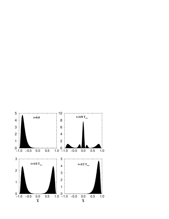
Figure 2: Probabity density plot of DOCS of symmetric-Pöschl-Teller potential at different times for $\beta=0.8$ and $\rho=10$.

Figure 3: Probabity density plot for AOCS of symmetric-Pöschl-Teller potential at different times for $\beta^{{}^{\prime}}=30$ and $\rho=10$.

Thus, at time $t=1/2\;T_{rev}$, a mirror image of the initial wave packet is produced at the opposite end of the potential well (Fig. 2 and 3). This can be observed as a bright ray at time $t=1/2\;T_{rev}$, in the quantum carpet structure (Fig. 4). The auto-correlation function

$$A(t)\;=\;\langle\chi(\bar{x},t)|\chi(\bar{x},0)\rangle,$$ (25)

yields

$$A(t=1/2)\;=\;\sum_{(A+n)\;even}|d_{n}|^{2}-\sum_{(A+n)\;odd}|d_{n}|^{2}\;.$$ (26)

Figure 4: (Colour Online) Quantum carpet of the displacement operator coherent state of symmetric-Pöschl-Teller potential for $\beta=0.8$ and $\;\rho=10$, brightness signifies the maximum.

As $d_{n}$ oscillates rapidly, it will not contribute significantly to the $|A(t)|^{2}$ (Fig. 5), at $t=1/2\;T_{rev}$. At time $t=1/4\;T_{rev}$ the CS wave packet becomes

$$\chi(\bar{x},\frac{1}{4}T_{rev}) = \frac{1}{\sqrt{2}}e^{-i\pi/4}\left[\chi(\bar{x},0)+e^{i\pi/2}\chi(-\bar{x},0)\right]$$

$$|\chi(\bar{x},\frac{1}{4}T_{rev})|^{2}\; = \frac{1}{2}\left[|\chi(\bar{x},0)|^{2}+|\chi(-\bar{x},0)|^{2}\right]$$ (27)

Figure 5: Plot of square modulus $|_{SPT}\langle\chi(x,t)|\chi(x,0.)\rangle_{SPT}|^{2}$ of the auto correlation function of DOCS as a function of time, for $\beta=0.8$, $\rho=10$.

In this case, the wave packet breaks up into two parts which are situated at the two opposite corners of the potential well (Fig. 2 and 3). This gives rise to two bright spots at the two vertical ends of the quantum carpet at $t=.25$. At the same instance, the auto-correlation function only gives a peak, as manifested in Fig. 5. To explain the probability density plot at $t=0.125$, we consider a fictitious classical wave packet

$$\chi_{cl}(\bar{x},t)\;=\;\sum_{n=0}^{\infty}\;\;d_{n}\;\psi_{n}(\bar{x})e^{-2\pi i\frac{n}{T_{cl}}t}\;,$$ (28)

which behaves like the initial wave packet at small time (order of $T_{cl}$) where $T_{cl}=\frac{2\pi}{\alpha^{2}\rho}$. Using the discrete Fourier transform (DFT), the original CS wave packet (Eq. (22)) at time $t=\frac{r}{s}T_{rev}$ can be written as a linear combination of classical wave packet of Eq. (28) as

$$\chi(\bar{x},\frac{r}{s}T_{rev})\;=\;\sum_{p=0}^{l-1}\;\;a_{p}\;\chi_{cl}(\bar{x},\frac{r}{s}T_{rev}+\frac{p}{l}T_{cl})\;,$$ (29)

where

$$a_{p}=\frac{1}{l}\;\sum_{n=0}^{l-1}\;\;\exp\left[2\pi i(n\frac{p}{l}-n^{2}\frac{r}{s})\right]\;.$$ (30)

Here, $r$ and $s$ are two mutually prime integers and $l$ is the period of the quadratic phase term. In general, $l=\frac{s}{2}$, if $s$ is integral multiple of $4$ and $l=s$ in all other cases. In this case $\frac{r}{s}=\frac{1}{8}$ and $l=\frac{s}{2}=4$, Substituting in Eq. (29) and Eq. (30), we get

$$\chi(\bar{x},\frac{1}{8}T_{rev})=\;a_{0}\;\chi_{cl}^{(0)}\;+\;a_{1}\chi_{cl}^{(1)}\;+\;a_{2}\chi_{cl}^{(2)}\;+\;a_{3}\chi_{cl}^{(3)}\;$$ (31)

where

$$\chi_{cl}^{(i)}=\chi_{cl}(\bar{x},\frac{1}{8}T_{rev}+\frac{i}{4}T_{cl}),\quad i=0,1,2,3\;$$ (32)

and $a_{0}=-a_{2}=\frac{1}{2\sqrt{2}}(1-i)\;$; $a_{1}=a_{3}=1/2$.

The above expression (31) signifies that the wave packet has broken into four parts, each of them differing by a phase $\pi/4$. In the probability density

$$|\chi(t=\frac{1}{8})|^{2}\; = \;\frac{1}{4}\left[|\chi_{cl}^{1}|^{2}\;+\;|\chi_{cl}^{2}|^{2}\;+\;|\chi_{cl}^{3}|^{2}\;+\;|\chi_{cl}^{4}|^{2}\right]$$ (34)

$$+\frac{1}{2}\textrm{Re}\left[{\chi_{cl}^{1}}^{*}\chi_{cl}^{2}e^{i\pi/4}-{\chi_{cl}^{1}}^{*}\chi_{cl}^{3}+{\chi_{cl}^{1}}^{*}\chi_{cl}^{4}e^{i\pi/4}\right.$$

$$\;-\left.{\chi_{cl}^{2}}^{*}\chi_{cl}^{3}e^{-i\pi/4}\;+{\chi_{cl}^{2}}^{*}\chi_{cl}^{4}-{\chi_{cl}^{3}}^{*}\chi_{cl}^{4}e^{i\pi/4}\right],$$

the first term carries the contribution from the individual subsidiary waves and the second term arises due to the interference between them. We note that the $\chi_{cl}^{1}$ and $\chi_{cl}^{3}$ are spatially well separated, giving very less contribution in interference. The dominant interference term is ${\chi_{cl}^{2}}^{*}\chi_{cl}^{4}$, as $\chi_{cl}^{2}$ and $\chi_{cl}^{4}$ are not spatially separated. Thus, at time $t=0.125$, wave function splits into four parts, but their interference at the middle gives a strong peak, rather than giving four distinct similar waves. For comparison, the wave packet structure for AOCS of symmetric-Pöschl-Teller potential is also shown in Fig. 3. In this case, as the initial wave packet is sharper, the interference terms are less dominant than that of DOCS.

We have observed that the initial wave packet remains in the left corner of the potential well and oscillates due to the impulse from the well and at later times, as it spreads, being away from the boundary of the well. This is quite transparent from the quantum carpet structure, which gives the space time rays of probability density of the corresponding coherent states. We note that, the rays in quantum carpet are not straight lines which is the case for infinite square-well.

In order to contrast the temporal evolution of the DOCS with the classical motion, we note that for a particle of energy $E$,

$$x(t)\;=\;a\;\arccos\left[\frac{\alpha_{1}-\beta_{1}}{2}+\sqrt{\Delta}\cos{(\sqrt{\frac{2E_{c}}{m}}\frac{t}{a})}\right]$$ (35)

where $\Delta=(1-\frac{1}{2}(\sqrt{\alpha_{1}}+\sqrt{\beta_{1}})^{2})(1-\frac{1}{2}(\sqrt{\alpha_{1}}-\sqrt{\beta_{1}})^{2})$, $V_{0}=\frac{\alpha^{2}}{m}$ and $\alpha_{1}=\frac{V_{0}}{E_{c}}\rho(\rho-1),\;\beta_{1}=\frac{V_{0}}{E_{c}}k(k-1)$; with the condition

$$E_{c}>\frac{V_{0}}{2}(\sqrt{\rho(\rho-1)}+\sqrt{k(k-1)})^{2}.$$ (36)

Figure 6: Plots of expectation values of x for (a) the coherent state of the Pöschl-Teller potential, with different values of $\beta$ where $\rho=5,k=5$ and $\alpha=2$.(b) classical solution of Pöschl-Teller potential, with $a=0.25,m=1,V_{0}=4,k=5,\rho=5$ and $E_{c}=$ average value of energy for $\beta=0.1$.

This classical trajectory is shown in Fig. 6(b). The expectation value of the position with respect to the coherent state of general trigonometric Pöschl-Teller potential is obtained as

$$\langle x(t)\rangle\;=\frac{1}{\alpha}\arcsin\sqrt{1/2\;(1-z)}$$ (37)

where

$$z=N\;\sum_{n=0}^{\infty}\;(2A_{n}\;\cos{\left[2\;\alpha^{2}(2n+\rho+k+1)t\right]-C_{n}})$$

having,

$$A_{n}=-(\beta)^{2n+1}\\ \left[\frac{2\Gamma{(\rho+n+3/2)}\Gamma{(k+n+3/2)}}{\Gamma{(\rho+k+n)}\Gamma{(n+1)}(2n+\rho+k)(2n+\rho+k+1)(2n+\rho+k+2)}\right]$$

and

$$C_{n}=(\beta)^{2n}\left[\frac{\Gamma{(\rho+n+1/2)}\Gamma{(k+n+1/2)}(k+\rho-1)(k-\rho)}{\Gamma{(\rho+k+n)}\Gamma{(n+1)}(2n+\rho+k)(2n+\rho+k-1)(2n+\rho+k+1)}\right]$$

N being the normalization constant. This $\langle x(t)\rangle$ is plotted in Fig. 6(a) which nearly matches with the classical trajectory for very small values of $\beta$ (solid line in Fig. 6(a)). In this case only a few eigen states contribute to the coherent state wave packet. Sudden changes in the $\langle x(t)\rangle$ values are the signatures of revivals and the fractional revivals [33].

5 Conclusions

In conclusion, the algebraic procedure used here, for constructing CSs for potentials based on confluent hypergeometric and hypergeometric differential equations depends on the fact that, the solutions of the above differential equations can be precisely connected with the space of monomials. This leads to a straightforward identification of symmetry generators, without taking recourse to additional angular variables or SUSY type multiple, related Hamiltonians. The nature of the specific potential enters through the corresponding ground states and by fixing the parameters and variables of the above solutions. We have concentrated here on the CS of Pöschl-Teller potential, since various potentials can be obtained from the same, through limiting of parameters and point canonical transformation. The time evolution of the CS for this potential, having non-linear spectra, produces cat like states in fractional revivals. We contrasted the properties of the two different types of CSs possible here, as well as the temporal evolution of the CS, with classical motion. As has been noted earlier, this procedure easily extends to more complicated non-linear coherent states arising from deformed algebras, a subject we intend to take up in future. We also would like to analyze the subject of mesoscopic superposition and sub-Planck scale structure [34], possible in this type of quantum systems.

6 References

References

- [1] Schrödinger E 1926 Naturwissenschaften 14 664
-
[2]
Glauber R J 1963 Phys. Rev. 130
2529
Glauber R J 1963 Phys. Rev. Lett. 10 84
Glauber R J 1963 Phys. Rev. 131 2766
Klauder J R 1963 J. Math. Phys. 4 1055
Klauder J R 1966 Phys. Rev. Lett. 16 534 - [3] Klauder J R and Skagerstam B S 1985 Coherent States: Applications in Physics and Mathematical Physics (World Scientific, Singapore)
-
[4]
Klauder J R 1996 J. Phys. A: Math. Gen. 29
L293
Gazeau J P and Klauder J R 1999 J. Phys. A: Math. Gen. 32 123
Antoine J P et al 2001 J. Math. Phys. 42 2349 and references therein - [5] Perelomov A M 1986 Generalized Coherent States and Their Applications (Springer, Berlin)
- [6] Zhang W M, Feng D H and Gilmore R 1990 Rev. Mod. Phys. 62 867 and references therein
- [7] Agarwal G S Selected Papers on Fundamentals of Quantum Optics (SPIE milestone series) 103.
-
[8]
Averbukh I Sh and Perelman N F 1989 Phys. Lett. A 139
449
Banerji J and Agarwal G S 1999 Phys. Rev. A 59 4777
Hall M J W, Raineker M S and Schleich W P 1999 J. Phys. A: Math. Gen. 32 8275
Kaplan A E et al2000 Phys. Rev. A 61 032101 - [9] Bluhm R, Kostelecky V A, and Porter J 1996 Am. J. Phys. 64 944
- [10] Doncheski M A and Robinett R W 2004 Phys. Rep. 392 and references therein
- [11] Tara K, Agarwal G S and Chaturvedi S 1993 Phys. Rev. A 47 5024
- [12] Nieto M M and Simmons Jr. L M 1978 Phys. Rev. Lett. 41 207
-
[13]
Benedict M G and Molnár B 1999 Phys. Rev. A 60 R1737
Dong S H 2002 Can. J. Phys. 80 129 - [14] Roy B and Roy P 2002 Phys. Lett. A 296 187.
-
[15]
Chenaghlou A and Fakhri H 2002Mod. Phys. Lett.
A 17 1701
Jellal A 2002Mod. Phys. Lett. A 17 671
Fakhri H and Chenaghlou A 2003 Phys. Lett. A 310 1 - [16] Shapiro E A, Spanner M and Ivanov M Y 2003 Phys. Rev. Lett. 91 237901
- [17] Nieto M M 1978 Phys. Rev. A 17 1273
-
[18]
Nieto M M and Simmons, Jr. L M 1979 Phys. Rev.
D 20 1332
Nieto M M and Simmons, Jr. L M 1979 Phys. Rev. D 20 1342 - [19] Crawford M G A and Vrscay E R 1998 Phys. Rev. A 57 106
- [20] Kinani A H and Daoud M 2001 Phys. Lett. A 283 291
- [21] Nieto M M 2001 Mod. Phys. Lett. A 16 2305
- [22] Hassouni Y, Curado E M F and Rego-Monteiro 2005 Phys. Rev. A 71 022104
-
[23]
Cooper F, Khare A and Sukhatme U P 1995 Phys.
Rep. 251 268
Cooper F, Khare A and Sukhatme U P 2001 Supersummetry in Quantum Mechanics (World Scientific, Singapore) -
[24]
Gangopadhyaya A, Mallow J V and
Sukhatme U P 1998 Phys. Rev. A 58 4287
Wu J and Alhassid Y 1990 J. Math. Phys. 31 557
Wu J, Alhassid Y and Gürsey F 1989 Ann. Phys. 196 163 - [25] Aleixo A N F and Balantekin A B 2004 quant-ph/0407160 and references therein
- [26] Shreecharan T, Panigrahi P K and Banerji J 2004 Phys. Rev. A 69 012102
- [27] Gurappa N, Panigrahi P K and Shreecharan T 2003 J. Comput. Appl. Math. 160 103
- [28] Loinaz W and Newman T J 1999 J. Phys. A: Math. Gen. 32 8889
- [29] Gurappa N and Panigrahi P K 2003 ibid. 67 155323
- [30] Shanta P et al1994 Phys. Rev. Lett. 72 1447
- [31] Quesne C 1999 J. Phys. A: Math. Gen. 32 6705
-
[32]
Gradshteyn I S and Ryzhik I M 2000 Table
of Integrals, Series and Products (Academic Press, USA)
Abramowitz M and Stegan I A 1970 Handbook of Mathematical Functions (Dover, New York) - [33] Sudheesh C, Lakshmibala S and Balakrishnan V 2004 Phys. Lett. A 329 14
- [34] Zurek W H 2001 Nature 412 712