Pulse retrieval and soliton formation in a non-standard scheme for dynamic electromagnetically induced transparency

Abstract

We examine in detail an alternative method of retrieving the information written into an atomic ensemble of three-level atoms using electromagnetically induced transparency. We find that the behavior of the retrieved pulse is strongly influenced by the relative collective atom-light coupling strengths of the two relevant transitions. When the collective atom-light coupling strength for the retrieval beam is the stronger of the two transitions, regeneration of the stored pulse is possible. Otherwise, we show the retrieval process can lead to creation of soliton-like pulses.

I Introduction

Recent progress in the coherent control of light-matter interactions has led to many interesting possibilities and practical applications. Amongst them is the concept of electromagnetically induced transparency (EIT), first proposed by Harris Harris1997 , in which a strong coherent field (“control”) is used to make an otherwise opaque medium transparent near atomic resonance for a second weak (“probe”) field. This EIT scheme can be used to store and retrieve the full quantum information in a weak probe field by changing the strength of the control field while the pulse is inside the atomic sample Fleischhauer2000 . In this paper we examine in detail an alternative method of retrieving the stored information that was first proposed by Matsko et al. Matsko2001 , and investigate the parameter regime under which this process is feasible.

The usual way of retrieving the stored information consists of a time-reversed version of the writing process Liu2001 ; Phillips2001 . The elegant physics behind this scheme was described by Fleischhauer and Lukin, who noted that the combined atomic and optical state adiabatically follows a dark state polariton Fleischhauer2002 . The “writing” process involves turning the control field to zero, storing the quantum information of the light beam as the purely atomic form of the polariton. When the control field is returned back to its original value, the polariton switches back to photonic form, identical to original optical pulse. In work describing some of the detailed behavior of that process, Matsko et al. noted an alternate scheme that may also store and reproduce a copy of a weak probe pulse Matsko2001 . In this scheme, the writing process remains the same, but retrieval of the pulse involves applying a coherent control field to the transition originally coupled by the probe field. This causes the probe pulse to be regenerated on the transition originally coupled by the control field. This alternative scheme cannot be explained in terms of dark state polaritons, and behaves quite differently for different parameters of the system. We analyze this scheme in detail in this paper.

As it is important to distinguish between the different control fields applied at different times, we will refer to the control field as the “writing” field during the first part of the process (storage) and as the “retrieval” field during the second part (the regeneration of the probe pulse).

We will show that when the collective atom-light coupling strength for the retrieval beam is the largest of the two transitions, retrieval is possible and the retrieved pulse is amplified, time reversed, stretched or compressed in time and phase conjugated compared to the input pulse. Conversely, if the collective coupling strength of the retrieval beam is not the largest of the two transitions, we find that the retrieved pulse differs substantially from the input pulse and the retrieval process can lead to the creation of a soliton-like combination of electromagnetic fields and atomic coherences that propagates without change in shape.

II Model

To analyze the system we use a quasi one-dimensional model, consisting of two copropagating pulses passing through an optically thick medium of length $l$ consisting of three-level atoms. The atoms have two metastable ground states $|b\rangle$ and $|c\rangle$ which interact with two fields $\hat{\mathcal{E}}_{p}(z,t)$ and $\hat{\mathcal{E}}_{c}(z,t)$ as shown in Figure 1. $\hat{\mathcal{E}}_{i}$ are the slowly varying amplitude related to the positive frequency part of the electric field given by

$$\hat{E}_{p}^{+} = \sqrt{\frac{\hbar\omega_{ab}}{2\epsilon_{0}V}}\hat{\mathcal{E}}_{p}(z,t)e^{\frac{i\omega_{ab}}{c}(z-ct)}$$

$$\hat{E}_{c}^{+} = \sqrt{\frac{\hbar\omega_{ac}}{2\epsilon_{0}V}}\hat{\mathcal{E}}_{c}(z,t)e^{\frac{i\omega_{ac}}{c}(z-ct)}.$$

Here $\omega_{\mu\nu}=(E_{\mu}-E_{\nu})/\hbar$ is the resonant frequency of the $|\mu\rangle\leftrightarrow|\nu\rangle$ transition and $V$ the quantization volume, here taken as the interaction volume. As the pulses are co-propagating we are able to neglect Doppler effects.

Figure 1: Level structure of the atoms

To perform a quantum analysis of the light-matter interaction it is useful to use locally-averaged atomic operators. We take a length interval $\delta z$ over which the slowly-varying field amplitudes do not change much, containing $n\mathcal{A}\delta z\gg 1$ atoms, where $n$ is the atomic density and $\mathcal{A}$ is the cross sectional area of the pulses, and introduce the continuous atomic operators

$$\hat{\sigma}_{\mu\nu}(z,t)=\frac{1}{n\mathcal{A}\delta z}\sum_{i,z\leq z_{i}<z+\delta z}|\mu^{i}(t)\rangle\langle\nu^{i}(t)|e^{\frac{i\omega_{\mu\nu}}{c}(z-ct)}.$$ (1)

where $z_{i}$ is the position of the $i$th atom and $|\mu^{i}(t)\rangle$ is the $|\mu\rangle$ state wavefunction for the $i$th atom..

Using these continuous atomic operators, the interaction Hamiltonian under the rotating wave approximation is given by

$$\hat{\mathcal{H}}=-\int_{0}^{l}\frac{N\hbar}{l}[g_{p}\hat{\mathcal{E}}_{p}(z,t)\hat{\sigma}_{ab}(z,t)+g_{c}\hat{\mathcal{E}}_{c}(z,t)\hat{\sigma}_{ac}(z,t)+H.c.]dz$$ (2)

where $l$ is the length of the cell, $N$ is the number of atoms in the interaction region and the coupling constants are $g_{p}=d_{ab}\sqrt{\omega_{ab}/2\epsilon_{0}V\hbar}$, $g_{c}=d_{ac}\sqrt{\omega_{ac}/2\epsilon_{0}V\hbar}$ where $d_{ab}$ and $d_{ac}$ are the dipole moments of the $|a\rangle\leftrightarrow|b\rangle$ and $|a\rangle\leftrightarrow|c\rangle$ transitions respectively. This Hamiltonian leads to the following equations of motion for the density matrix elements and fields

$$\dot{\rho}_{bb} = \gamma_{b}\rho_{aa}-i\Omega_{p}\rho_{ba}+i\Omega_{p}^{\ast}\rho_{ab}$$ (3)

$$\dot{\rho}_{cc} = \gamma_{c}\rho_{aa}-i\Omega_{c}\rho_{ca}+i\Omega_{c}^{\ast}\rho_{ac}$$

$$\dot{\rho}_{ab} = -\gamma_{ab}\rho_{ab}+i\Omega_{p}(\rho_{bb}-\rho_{aa})+i\Omega_{c}\rho_{ab}$$

$$\dot{\rho}_{cb} = -i\Omega_{p}\rho_{ca}+i\Omega_{c}^{\ast}\rho_{ab}$$

$$\dot{\rho}_{ca} = -\gamma_{ca}\rho_{ca}-i\Omega_{p}^{\ast}\rho_{cb}+i\Omega_{c}^{\ast}(\rho_{aa}-\rho_{cc})$$

$$\left(\frac{\partial}{\partial t}\right. + \left.c\frac{\partial}{\partial z}\right)\Omega_{p}=i\alpha_{p}\rho_{ab}$$

$$\left(\frac{\partial}{\partial t}\right. + \left.c\frac{\partial}{\partial z}\right)\Omega_{c}=i\alpha_{c}\rho_{ac}$$ (4)

where the $\gamma_{\mu}$ are phenomenological decay rates and we have defined the two Rabi frequencies as $\Omega_{i}=g_{i}\langle\hat{\mathcal{E}}_{i}\rangle$ and the constants $\alpha_{p}=N|g_{p}|^{2}$ and $\alpha_{c}=N|g_{c}|^{2}$ are the collective atom-light coupling constants for the transitions $|b\rangle\leftrightarrow|a\rangle$ and $|c\rangle\leftrightarrow|a\rangle$ respectively.

We now proceed to consider the modified version Matsko2001 ; Zibrov2002 of the storage and retrieval scheme using dynamic EIT. With all the atoms initially optically pumped into the ground state $|b\rangle$, we turn on the writing beam driving the $|c\rangle\leftrightarrow|a\rangle$ transition to its maximum value $\Omega_{c}^{0}$, while a small input pulse of maximum amplitude $\Omega_{p}^{0}\ll\Omega_{c}^{0}$ is sent into the medium on the $|b\rangle\leftrightarrow|a\rangle$ transition. EIT effects cause the group velocity of the the input pulse to be drastically reduced to a new value given by Fleischhauer2002

$$v_{g}=\frac{c}{1+\alpha_{p}/|\Omega_{c}^{0}|^{2}}$$ (5)

which can be much less than the speed of light. This leads to significant spatial compression of the input pulse as it enters the medium, allowing the entire pulse (the typical pulse length outside the cell is of order of a few kilometers) to be stored inside a vapor cell (of length a few centimeters). Once the input pulse is completely inside the medium, we slowly turn off the writing beam on the $|c\rangle\leftrightarrow|a\rangle$ transition. This writes the information carried by the input pulse onto a collective atomic coherence for storage Fleischhauer2002 .

After a controllable storage time $T_{s}$, the stored information can be retrieved by turning on a retrieval beam driving the $|b\rangle\leftrightarrow|a\rangle$ transition as proposed in Matsko2001 ; Zibrov2002 . Note that this is in contrast to the usual retrieval scheme for EIT light storage in which the retrieval beam is on the $|c\rangle\leftrightarrow|a\rangle$ transition and the output pulse is generated on the $|b\rangle\leftrightarrow|a\rangle$ transition Fleischhauer2002 . For normal EIT in the ideal case, the output pulse is identical to the input pulse. Here, because the time reversed version of the writing beam is on the $|b\rangle\leftrightarrow|a\rangle$ transition, the output pulse is generated on the $|c\rangle\leftrightarrow|a\rangle$ transition. As a consequence the output pulse need not have the same frequency or polarization as the input pulse.

It is not immediately clear why any fields made by this process would be correlated with the stored pulse. After all, the original pulse produces a small population in state $|c\rangle$ and leaves most atoms in state $|b\rangle$, so the control beam is mainly interacting with states that have not been affected by the original pulse in any significant way. Also, as the strong retrieval beam is initiated on the most populated transition, it will lead to significant spontaneous emission, which would appear to dominate any kind of coherent process necessary for the retrieval. However, as will be shown later, our simulation indicates that under some parameter regimes, it is indeed possible to recover an output related in amplitude and phase to the input pulse.

III Retrieving the probe pulse

We will start with an example that illustrates a successful pulse retrieval, and then go on to analyze other possible behaviors of this system. We assume standard atomic initial conditions for EIT given by $\rho_{bb}(z,0)=1$; $\rho_{cc}(z,0)=\rho_{ab}(z,0)=\rho_{cb}(z,0)=\rho_{ca}(z,0)=0$. In order to better identify the properties of the new retrieval scheme and to judge the quality of the retrieval process, we choose an input pulse at $z=0$ to be the sum of two Gaussians of different height (so the total input pulse is non-symmetric) with a time-varying phase factor. The boundary conditions for the fields at $z=0$ is of the form

$$\Omega_{p}(0,t) = \Omega_{p}^{0}f(t)e^{if(t)}+\frac{\Omega_{c}^{0}}{2}\left[1+\tanh\left(\frac{t-T_{on}}{T_{s}}\right)\right]$$ (6)

$$\Omega_{c}(0,t) = \frac{\Omega_{c}^{0}}{2}\left[1-\tanh\left(\frac{t-T_{off}}{T_{s}}\right)\right]$$ (7)

where $f(t)$ is a unit amplitude envelope function. The first part of equation (6) describes the input (signal) pulse that we wish to store, whereas the second part of equation (6) describes the turning on of the retrieval beam (amplitude $\Omega_{c}^{0}$) at time $T_{on}$ with a switching time of approximately $T_{s}$. $\Omega_{c}$ describes the turning off of the writing beam at time $T_{\mbox{\it off}}$. These boundary conditions for the fields are plotted in Figure 2.

With these initial conditions, the equations of motion (4) can be solved numerically in the moving frame defined by $\xi=z$, $\tau=t-z/c$ using the method described in Shore Shore implementing the numerical integration with a fourth order Runge-Kutta method XMDS . For convenience, we choose $\gamma_{b}=\gamma_{ab}=\gamma$ and $\gamma_{c}=\gamma_{ca}=(\alpha_{c}/\alpha_{p})\gamma$.

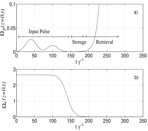
Figure 2: Envelope of pulses entering the medium at $z=0$ as a function of time. a) $\Omega_{p}$ is the field driving the $|b\rangle\leftrightarrow|a\rangle$ transition and b) $\Omega_{c}$ is the field driving the $|c\rangle\leftrightarrow|a\rangle$ transition. The parameters are $T_{\mbox{\it off}}=140\gamma^{-1}$, $T_{s}=18.85\gamma^{-1}$, $T_{on}=259\gamma^{-1}$, $\Omega_{p}^{0}=0.0265\gamma$ and $\Omega_{c}^{0}=2.6526\gamma$. Amplitude of pulses are displayed in units of $\gamma$. The input pulse to be stored is $\Omega_{p}$ before the start of storage. The retrieved pulse is $\Omega_{c}$ after the storage process.

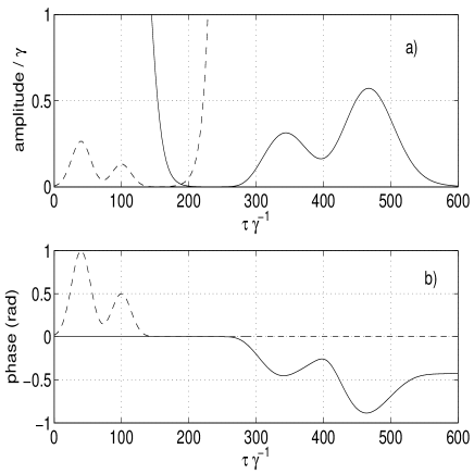
Figure 3: Comparison of a) amplitude and b) phase of both the retrieved and input pulses. The solid line represents the retrieved pulse and the dashed line the input pulse (magnified by a factor of ten). The parameters are $\alpha_{p}=30177\gamma$, $\alpha_{c}=29272c\gamma$, $l=4$cm. The input pulses are as shown in Figure 2. The large amplitude on the retrieval pulse transition at earlier times is because the field on this transition was used as the writing beam initially. Similarly the large value on the input pulse transition at later times represents the retrieval beam.

Figure 3 shows a comparison of the phase and amplitude of the retrieved and input pulses, both propagating in the positive $z$ direction. In practice, this output pulse of well-defined shape will be superimposed on top of spontaneously emitted photons, so for the purposes of observing this output, it would be better to choose the lowest atomic density allowed for EIT to work.

From the graphs, we observe that the retrieved pulse is time reversed, amplified, widened in time and is the phase conjugate of the input pulse. We can understand this behavior by examining the interaction of the retrieval beam with the stored coherence and how the retrieved pulse is generated. As the writing part of our process is identical to the usual dynamic EIT setup Fleischhauer2002 , we know that at the end of the storage process, the only variable of the system aside from $\rho_{bb}$ that is significantly nonzero is $\rho_{cb}$ whose spatial variation, shown in Figure 4, encodes the phase and amplitude information of the original input pulse.

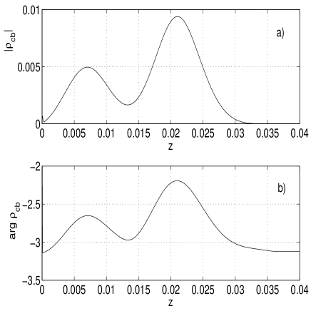
Figure 4: Amplitude a) and phase b) of $\rho_{cb}$ during storage.

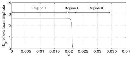
Figure 5: Spatial variation of the retrieval beam divides the medium into three regions as described in the text. At any time, the retrieved pulse is generated due to the dynamics that occur in region II where the retrieval beam is in the process of pumping population out of state $|b\rangle$. In region I, all atoms are in state $|c\rangle$. The beam has not yet penetrated to region III.

The retrieval beam enters the medium driving the transition $|b\rangle\leftrightarrow|a\rangle$ while almost all the atoms are in state $|b\rangle$. As the medium is optically thick, the retrieval beam is strongly absorbed and its initial wavefront moves across the medium at a speed much less than the speed of light. The spatial variation of the retrieval beam at any time during the retrieval process has the general shape shown in Figure 5. At any time, this shape divides the medium into three regions with distinct dynamics. In region I, the retrieval beam $\Omega_{p}$ has attained its maximum value as it has optically pumped all atoms into the state $|c\rangle$. In region II, the wavefront of the retrieval beam is severely attenuated due to absorption and in region III, not yet reached by the retrieval beam, all the atoms are still in the polariton state left by the writing process. This means that most of the atoms are in state $|b\rangle$ here. We note that at any point in time, the interesting dynamics related to the retrieval of the stored information is occurring only in region II. In this region the retrieval beam $\Omega_{p}$ is in the process of pumping atoms from $|b\rangle$ to $|a\rangle$ at a rate of $|\Omega_{p}|^{2}/\gamma$. Before a significant population has accumulated in $|c\rangle$, the retrieval beam can coherently scatter off the stored coherence $\rho_{cb}$, generating a retrieved pulse on the $|a\rangle$ to $|c\rangle$ transition. These generated photons will encode some of the properties of the input pulse and propagate out of the medium at the speed of light through region III, as this region contains only atoms in $|b\rangle$.

On long time-scales optical pumping alters $\rho_{cb}$ and will overwrite any coherence that was initially stored there. At this point, photons emitted when atoms decay from $|a\rangle$ to $|c\rangle$ will bear no relation to the input pulse. Furthermore, any field on the $|c\rangle\leftrightarrow|a\rangle$ transition will be strongly damped due to the significant population in state $|c\rangle$.

Note that in contrast to the adiabatic following in the usual EIT procedure Fleischhauer2002 , the retrieval process here is non-adiabatic and as demonstrated in Figure 6(a), the population in the excited state $|a\rangle$ can be quite significant during the retrieval process.

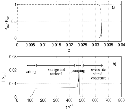
Figure 6: a) $\rho_{cc}$ (dashed) and $\rho_{aa}$ (solid) as a function of $z$ during the retrieval process. A significant population resides in the excited state during the retrieval process. b) $|\rho_{cb}(0.024,\tau)|$ as a function of $\tau\gamma^{-1}$. The spike in the graph shows the effect of optical pumping by the retrieval beam which overwrites the stored coherence.

Using this description of the dynamics, one can explain many of the features exhibited by the retrieved pulse. The time reversal occurs because the wavefront of the retrieval beam moves slowly from left to right, so the part of the stored coherence that is closest to the cell entrance sees the retrieval beam first. This part of the coherence near the medium entrance corresponds to the tail end of the input pulse (i.e. the part of the input pulse that entered the cell last), so the tail end of the input pulse will be retrieved first, resulting in an output that is time reversed. Figure 3 also demonstrates that the retrieved pulse can be amplified, and in this particular example the amplitude is increased by a factor of about twenty. This occurs because the new retrieval scheme has a larger reservoir of atoms available for producing photons. In the normal EIT setup photon number in the retrieved pulse is limited by the number of atoms in state $|c\rangle$ during the storage process which is strictly less than the number of photons in the input pulse. In this scheme the number of photons generated is limited by the maximum number of atoms in state $|c\rangle$ that the medium can sustain without destroying the stored coherence. This is a property of both the size of the stored coherence and the medium (e.g. optical density). It is, however, independent of the properties of the retrieval beam. For an optically dense medium, this is generally much larger than the number of photons in the input pulse.

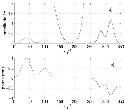
Figure 7: Comparison of a) amplitude and b) phase of retrieved (solid) and input (dashed) pulses. The input pulse has been magnified by a factor of ten. The amplitude of the retrieval beam is now $\Omega_{p}^{0}=5.3052\gamma$ twice the value in Figure 3. We see that the retrieved pulse is made earlier in time and narrower in time because of the increased pumping rate by the retrieval beam. All other parameters are identical to those in Figure 3.

It is also clear that the width of the retrieved pulse is determined by the speed at which the wavefront of the retrieval beam propagates across the medium and not the initial pulse length. Figure 7 shows the retrieved pulse when the amplitude of the retrieval beam is doubled compared to Figure 3 while keeping all other parameters identical. We see that the output pulse is narrower and its amplitude larger while the total number of photons (as indicated by the area underneath the graph of intensities) remains approximately the same. This is due to the the more intense retrieval beam now being able to pump atoms out of $|b\rangle$ at a higher rate, enabling it to move across the medium more quickly and ensuring a shorter time interval between the retrieval of the front and back part of the original input pulse. Since the total number of generated photons is unaffected by the intensity of the retrieval beam, energy conservation necessitates that the retrieved pulse has greater amplitude.

The phase conjugation of the output pulse is most easily understood by examining the equations of motion (4) and (3). On a short time scale, we have $\rho_{bb}\approx 1\gg\rho_{cc},\rho_{aa}$, and the following set of equations describes the generation of the retrieved pulse from the conjugate of the stored coherence $\rho_{cb}^{\ast}$

$$\left(\frac{\partial}{\partial t}\right. + \left.c\frac{\partial}{\partial z}\right)\Omega_{c}=i\alpha_{c}\rho_{ac}$$ (8)

$$\rho_{ac}(z,t) = i\int_{T_{on}}^{t}e^{-\gamma(t-s)}\Omega_{p}(z,s)\rho_{cb}^{\ast}(z,s)ds.$$ (9)

Since $\rho_{cb}^{\ast}$ stores the conjugate of the input phase, the retrieved pulse is therefore the phase conjugate of the input pulse.

From examining the phase of the generated output field compared to the input, it is clear that the quality of the retrieval process, (in terms of extracting a pulse of the same shape as the time reversed input) is not perfect. For example, from Figure 3 (b), we see that the phase of the retrieved pulse fails to decay to zero after a certain time. This feature is even more prominent when we set the collective atom-light coupling constants to be equal $\alpha_{p}=\alpha_{c}$, as shown in Figure 8. Again we see that the phase of the retrieved pulse plateaus, this time near the peak of the second Gaussian. Increasing $\alpha_{c}$ further to move into the regime $\alpha_{c}>\alpha_{p}$, we see from Figure 9 that the quality of the retrieval process is so bad that the output pulse does not even display the characteristic double peak of the input pulse.

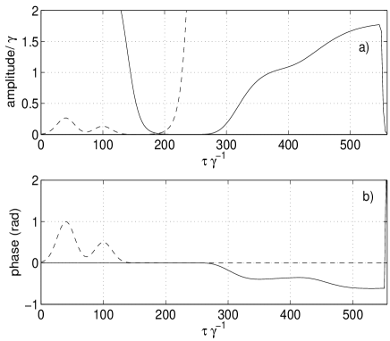
Figure 8: Comparison of a) amplitude and b) phase of retrieved (solid) and input (dashed) pulses. The input pulse has been magnified by a factor of ten. The abrupt cut off of the retrieved pulse near $\tau\gamma^{-1}=600$ is due to the arrival of the retrieval beam at the exit of the cell $z=0.04$ which pumps all atoms into state $|c\rangle$ and prevents any field existing on this transition. The parameters are $\alpha_{p}=\alpha_{c}=30177\gamma$, $l=4$cm. The input pulses are as given in Figure 2

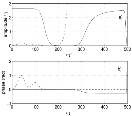
Figure 9: Comparison of a) amplitude and b) phase of retrieved (solid) and input (dashed) pulses. The input pulse has been magnified by a factor of ten. The parameters are $\alpha_{p}=30177c\gamma$ ¡ $\alpha_{c}=31082c\gamma$, $l=4$cm. The input pulses are as given in Figure 2.

To further investigate the behavior of the retrieved pulse as the relative strength of the collective coupling constant is varied, we consider a Gaussian input envelope as this makes clearer the difference in retrieval quality. Figure 10 show the three cases $\alpha_{p}>\alpha_{c}$, $\alpha_{p}=\alpha_{c}$, and $\alpha_{p}<\alpha_{c}$.

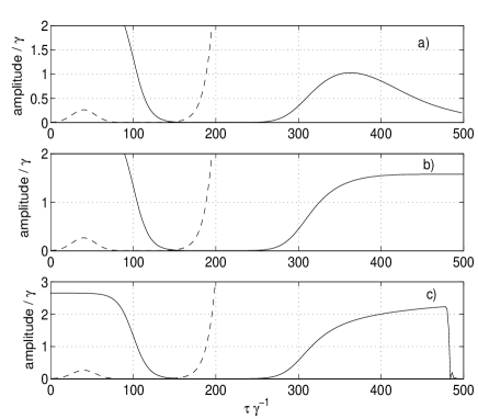
Figure 10: Comparison of amplitudes of input pulse (dashed) magnified by a factor of ten and output pulse (solid) for the three parameter regimes $\alpha_{p}>\alpha_{c}$ (a), $\alpha_{p}=\alpha_{c}$ (b) and $\alpha_{p}<\alpha_{c}$.

For $\alpha_{p}>\alpha_{c}$, the generation of the output pulse automatically ceases so that the retrieved pulse will always display the falling end of the Gaussian input. However, as $\alpha_{c}$ approaches the value of $\alpha_{p}$, the pulse generation takes a longer time to cease giving the assymetric long tail shape shown in Figure 10 (a). When $\alpha_{p}=\alpha_{c}$, eventually a constant value of the generated field is maintained until the retrieval beam reaches the exit of the cell and pumps all the atoms to $|c\rangle$. Continuing the trend, Figure 10 (c) shows that in the regime of $\alpha_{p}<\alpha_{c}$, the generated pulse amplitude grows until the retrieval beam has optically pumped all the atomic population into $|c\rangle$. The phase variation of the retrieved pulse confirms the general trend that quality of the retrieval process decreases as we move across the three parameter regimes.

IV Soliton-Like Behavior

Our numerical results strongly indicate the existence of a soliton solution at the critical point $\alpha_{p}=\alpha_{c}$. At this point the field $\Omega_{c}$ generated from the stored coherence is able to induce a nonzero coherence $\rho_{cb}$ by a co-operative action with the retrieval beam $\Omega_{p}$. The induced $\rho_{cb}$ in turn can then be used to generate $\Omega_{c}$. This steady state cycling action explains why the system can continue to generate an output even when the ’dynamic’ region (region II in Figure 5) has moved beyond where the input pulse was originally stored. More specifically, when $\alpha_{p}>\alpha_{c}$, the induced coherence is not large enough to maintain the cycling action, causing the effect to die out; if $\alpha_{p}=\alpha_{c}$, the effect is self sustaining where the induced $\rho_{cb}$ is just sufficient to maintain the value of $\Omega_{c}$ that generated it; and for $\alpha_{p}<\alpha_{c}$, a greater coherence ($\rho_{cb}$) is induced, leading to an output at the cell exit that is continually amplified in time until cut off by the arrival of the retrieval beam. However, we have observed that when the cell length is increased, the amplitude of the output pulse appears to tend to a limiting value.

Figure 11 shows the induced $\rho_{cb}$, $\Omega_{p}$ and $\Omega_{c}$ for $\alpha_{p}=\alpha_{c}$ when the initially stored coherence no longer exists. We note that the shape and size of $\rho_{cb}$ and the fields propagate unchanged across the cell, indicating behavior characteristic of solitons. We also found that the shape and size of the final output is independent of the values of the coherences originally stored, indicating that the final field-coherence formation is a characteristic of the system independent of the storage/retrieval process requiring an initial nonzero $\rho_{bc}$ coherence only as a seed.

To demonstrate analytically that our results are in fact solitons we substitute the ansatz $\Omega_{i}(z,t)=\Omega_{i}(z-vt)$, $\rho_{\mu\nu}(z,t)=\rho_{\mu\nu}(z-vt)$ into equations (4) for the case $\alpha_{p}=\alpha_{c}$, where $v$ is the soliton parameter that designates the constant speed with which the soliton propagates across the medium. This allows us to determine the following relationship between the two pulses and the coherence generated as

$$\rho_{cb}(s)=-\frac{c-v}{\alpha_{0}v}\Omega_{p}(s)\Omega_{c}^{\ast}(s)$$ (10)

where $\alpha_{p}=\alpha_{c}=\alpha_{0}$ is the collective light-atom coupling constant identical for both transitions and $s=z-vt$. We also obtain the following relationship between the limiting values of the two fields

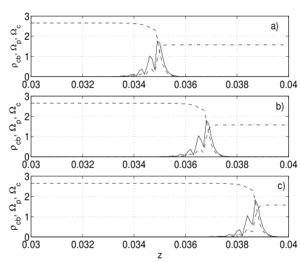
Figure 11: $|\Omega_{p}|$ (dash), $|\Omega_{c}|$ (dash-dot) and $|\rho_{cb}|\times 5$ (solid) as a function of $z$ at times $\tau\gamma^{-1}=477.6$ (a), $489$ (b), $501.6$ (c) for $\alpha_{p}=\alpha_{c}$ case. The field and atomic coherence propagates together unchanged across the cell

$$\frac{c-v}{\alpha_{0}v}(|\Omega_{p}^{\infty}|^{2}+|\Omega_{c}^{\infty}|^{2})=2$$ (11)

where $\Omega_{p}^{\infty}=\lim_{s\rightarrow-\infty}\Omega_{p}(s)$ and $\Omega_{c}^{\infty}=\lim_{s\rightarrow\infty}\Omega_{c}(s)$. When we compare equations (10) and (11) against the results of our numerics for various soliton parameters (the soliton parameter can be changed by varying the amplitude of the retrieval beam), we find good agreement. After further elimination of all the atomic variables, we obtain the two soliton equations relating the two fields

$$v\left[\Omega_{p}\frac{d^{2}\Omega_{c}^{\ast}}{ds^{2}}-\Omega_{c}^{\ast}\frac{d^{2}\Omega_{p}}{ds^{2}}\right]-\gamma\left[\Omega_{p}\frac{d\Omega_{c}^{\ast}}{ds}\right. - \left.\Omega_{c}^{\ast}\frac{d\Omega_{p}}{ds}\right]$$

$$=-\Omega_{p}\Omega_{c}^{\ast}\left(\frac{|\Omega_{p}^{\infty}|^{2}}{v}\right. - \left.\frac{\alpha_{0}}{c-v}\right)$$ (12)

$$-\Omega_{p}\left(v\frac{d^{3}\Omega_{p}}{ds^{3}}-\gamma\frac{d^{2}\Omega_{p}}{ds^{2}}\right) + \left(\frac{d\Omega}{ds}+\frac{2\gamma\Omega_{p}}{v}\right)\left(v\frac{d^{2}\Omega_{p}}{ds^{2}}-\gamma\frac{d\Omega_{p}}{ds}\right)$$ (13)

$$= \frac{2\Omega_{p}^{2}}{v}\frac{d}{ds}\left(|\Omega_{c}|^{2}+|\Omega_{p}|^{2}\right)$$

$$+ \frac{\gamma}{v^{2}}\Omega_{p}^{2}(|\Omega_{p}^{\infty}|^{2}-|\Omega_{c}|^{2}-|\Omega_{p}|^{2})$$

from which the dispersive and nonlinear terms are clearly visible.

We believe the photons generated from the cycling action outlined above bear little relation to the input pulse and are therefore not useful as far as quantum information retrieval is concerned. However the existence of the soliton-like solution and its sensitivity with respect to the coupling parameters is likely to lead to other interesting possibilities. A further analysis of the generation and properties of the solitons is beyond the scope of this paper, although the possibility that solitons can exist in atomic $\Lambda$ systems has previously been considered Rybin2004 ; Konopnicki1981

In conclusion, we have demonstrated the feasibility of an alternative retrieval scheme for dynamic EIT under certain parameter regimes and provided physical explanations for its behavior. Our numerical simulation also demonstrated the ability of this new scheme to create soliton-like features that are sensitive to the relative coupling strength of the two transitions. Due to its sensitivity to parameter change, we believe this solitonic behavior could prove useful within the context of magnetometry or high precision measurement.

We thank Elena Ostrovskaya for helpful discussions regarding the soliton features.

References

- (1) S. E. Harris Phys. Today 50 36 (1997)
- (2) M. Fleischhauer and M. D. Lukin, Phys. Rev. Lett. 84, 5094 (2000)
- (3) A. B. Matsko, Y. V. Rostovtsev, O. Kocharovskaya, A. S. Zibrov and M. O. Scully, Phys. Rev. A 64 043809 (2001)
- (4) C. Liu, Z. Dutton, C. Behroozi and L. V. Hau, Nature 409 490 (2001)
- (5) D. F. Phillips, A. Fleischhauer, A. Mair, R. L. Walsworth, and M. D. Lukin, Phys. Rev. Lett. 86 783 (2001)
- (6) M. Fleischhauer and M. D. Lukin, Phys. Rev. A 65, 022314 (2002)
- (7) A. S. Zibrov, A. B. Matsko, O. Kacharovskaya, Y. V. Rostovstsev, G. R. Welch and M. O. Scully, Phys. Rev. Lett. 88 103601 (2002)
- (8) B. W. Shore, The Theory of Coherence Atomic Excitation Wiley New York 1990
- (9) G. Collecutt, P.D. Drummond, P. Cochrane and J. J. Hope, ”Extensible Multi-Dimensional Simulator,” documentation and source available from http://www.xmds.org
- (10) A. V. Rybin and I. P. Vadeiko J. Opt. B 6 416 (2004)
- (11) M. J. Konopnicki and J. H. Eberly Phys. Rev. A 24 2567 (1981)