Scaling of non-Markovian Monte Carlo wave-function methods

Abstract

We demonstrate a scaling method for non-Markovian Monte Carlo wave-function simulations used to study open quantum systems weakly coupled to their environments. We derive a scaling equation, from which the result for the expectation values of arbitrary operators of interest can be calculated, all the quantities in the equation being easily obtainable from the scaled Monte Carlo wave-function simulations. In the optimal case, the scaling method can be used, within the weak coupling approximation, to reduce the size of the generated Monte Carlo ensemble by several orders of magnitude. Thus, the developed method allows faster simulations and makes it possible to solve the dynamics of the certain class of non-Markovian systems whose simulation would be otherwise too tedious because of the requirement for large computational resources.

I Introduction

The description of the dynamics of open quantum systems has attracted increasing attention during the last few years Breuer02a . The major reason for this is the identification of the phenomena of decoherence and dissipation, which characterize the dynamics of open quantum systems interacting with their surroundings Joos03a , as a main obstacle to the realization of quantum computers and other quantum devices Nielsen00a . Secondly, recent experiments on engineering of environments Myatt00a have paved the way to new proposals aimed at creating entanglement and superpositions of quantum states exploiting decoherence and dissipation Poyatos96a ; Plenio02a .

A common approach to the dynamics of open quantum systems consists in deriving a master equation for the reduced density matrix which describes the temporal behavior of the open system. The solution for the master equation can then be searched by using analytical or simulation methods, or the combination of both.

This article concentrates on the developing of new Monte Carlo simulation methods for non-Markovian open quantum systems. The general feature of the Monte Carlo methods is the generation of an ensemble of stochastic realizations of the state vector trajectories. The density matrix and the properties of the system of interest are then consequently calculated as an appropriate average of the generated ensemble.

Some common variants of the Monte Carlo methods for open systems include the Monte Carlo wave-function (MCWF) method Dalibard92a ; Molmer96a , the quantum state diffusion (QSD) Gisin92a ; Diosi98a ; Strunz99a , and the non-Markovian wave function (NMWF) formulation unravelling the master equation in an extended Hilbert space Breuer02a ; Breuer99a ; Breuer04a . The MCWF method has been very successfully used to model the laser cooling of atoms. Actually, 3D laser cooling has so far been described only by MCWF simulations Molmer95a . QSD in turn has been found to have a close connection to the decoherent histories approach to quantum mechanics Diosi95a , and NMWF method has been recently applied to study the dynamics of quantum Brownian particles Maniscalco04a ; Maniscalco04c . The various Monte Carlo methods and related topics have been reviewed e.g. in Refs. Molmer96a ; Carmichael93a ; Gardiner96a ; Plenio98a

In general, simulating open quantum systems is a challenging task. It has been shown earlier that the methods mentioned above can solve a wide variety of problems. Nevertheless, sometimes there arise situations in which the complexity of the studied system or the parameter region under study makes the requirement for the computer resources so large that the solution may become impossible in practice, though not in principle. Thus, it is important to assess the already existing methods from this point of view, and develop new variants to improve their applicability. This is the key point of this article.

Here, we address the Monte Carlo simulation methods for the short time-evolution of non-Markovian systems which are weakly coupled to their environments. In this case, the dynamics of the system may exhibit rich features, whereas the weak coupling may lead to extremely small quantum jump probabilities, the consequence being unpractically large requirement for the size of the generated Monte Carlo ensemble. To overcome this problem, we present below a method which in general allows to reduce the ensemble size.

By studying the Hilbert space path integral for the propagator of a piecewise deterministic process (PDP) Breuer02a , we show that part of the expectation value of an arbitrary operator $A$ as a function of time $t$, $\langle A\rangle(t)$, has scaling properties which can be exploited in Monte Carlo simulations to speed up the generation of the ensemble, in the optimal case by several orders of magnitude. We derive a scaling equation, from which the result for $\langle A\rangle(t)$ can be calculated, all the quantities in the equation being easily obtainable from the scaled Monte Carlo simulations.

We concentrate first on the Lindblad-type non-Markovian case which can be solved by the standard MCWF method, and then focus on the non-Lindblad-type case which requires the use of the NMWF simulations in the doubled Hilbert space.

The paper is structured as follows. Section II introduces the master equation, the corresponding stochastic Schrödinger equation, and the appropriate simulation schemes for the Lindblad- and non-Lindblad-type systems. The Hilbert space path integral method is then used to calculate the expectation value of an arbitrary operator setting the scene for the scaling method which is presented in Sec. III. Section IV shows explicitly how the scaling can be implemented and demonstrates the usability of the method, for the example of quantum Brownian motion. Finally Sec. V presents discussion and conclusions.

II Dynamics of non-Markovian systems

We describe first in Sec. II.1 the master equation for the Lindblad-type systems and the corresponding standard MCWF method. We then continue in Sec.II.2 with the description of the non-Lindblad-type case with the corresponding stochastic Schrödinger equation and NMWF unravelling in the doubled Hilbert space. The last subsection II.3 presents the calculation of the expectation value of an arbitrary operator $A$ with the Hilbert space path integral method which paves the way for the scaling procedure.

We begin by considering master equations obtained from the time-convolutionless projection operator technique (TCL) of the form Breuer02a ; Breuer99a

$$\frac{\partial}{\partial t}\rho\left(t\right) = A\left(t\right)\rho\left(t\right)+\rho\left(t\right)B^{{\dagger}}\left(t\right)$$ (1)

$$+\sum_{i}C_{i}\left(t\right)\rho\left(t\right)D^{{\dagger}}_{i}\left(t\right),$$

with time-dependent linear operators $A\left(t\right)$, $B\left(t\right)$, $C_{i}\left(t\right)$, and $D_{i}\left(t\right)$.

II.1 Lindblad-type case: master equation and MCWF method

A specific case of the master equation (1) is the one of Lindblad-type Gorini76a ; Lindblad76a ; Maniscalco04b

$$\frac{d}{dt}\rho(t) = -i\left[H_{S},\rho(t)\right]+\sum_{i}\gamma_{i}(t)\bigg{\{}L_{i}\rho(t)L_{i}^{\dagger}-$$ (2)

$$\left.\frac{1}{2}L_{i}^{\dagger}L_{i}\rho(t)-\frac{1}{2}\rho(t)L_{i}^{\dagger}L_{i}\right\},$$

where $H_{S}$ is the system Hamiltonian, $\gamma_{i}(t)$ the time dependent decay rate to channel $i$, and $L_{i}$ is the corresponding Lindblad operator.

We define this non-Markovian master equation to be of Lindblad-type when the time dependent decay coefficients $\gamma_{i}(t)\geq 0$ for all times $t$, and non-Lindblad type when $\gamma_{i}(t)$ acquire temporarily negative values during the time-evolution Maniscalco04b . The Lindblad-type case can be treated with the standard MCWF method introduced in this subsection Dalibard92a , and the non-Lindblad case with the NMWF method in the doubled Hilbert space presented in the following subsection Breuer99a ; Breuer02a .

The core idea of the standard MCWF method is to generate an ensemble of realizations for the state vector $\psi(t)$ by solving the time dependent Schrödinger equation

$$i\hbar\frac{\partial\psi(t)}{\partial t}=H(t)\psi(t),$$ (3)

with the non-Hermitian Hamiltonian $H(t)$

$$H(t)=H_{S}(t)+H_{DEC}(t),$$ (4)

where $H_{S}(t)$ is the reduced system’s Hamiltonian and the non-Hermitian part $H_{DEC}(t)$ includes the sum over the various allowed decay channels $i$,

$$H_{DEC}(t)=-\frac{i\hbar}{2}\sum_{i}\gamma_{i}(t)L_{i}^{\dagger}L_{i},$$ (5)

where the jump operator $L_{i}$ for channel $i$ coincides with the Lindblad operator appearing in the master equation (2).

During a discrete time evolution step of length $\delta t$ the norm of the state vector may shrink due to $H_{DEC}$. The amount of shrinking gives the probability of a quantum jump to occur during the short interval $\delta t$. Based on a random number one then decides whether a quantum jump occurred or not. Before the next time step is taken, the state vector of the system is renormalized. If and when a jump occurs, one performs a rearrangement of the state vector components according to the jump operator $L_{i}$, before renormalization of $\psi$.

The jump probability corresponding to the decay channel $i$ for each of the time-evolution steps $\delta t$ is

$$P_{i}(t)=\delta t\gamma_{i}(t)\langle\psi|L_{i}^{\dagger}L_{i}|\psi\rangle.$$ (6)

The expectation value of an arbitrary operator A is then the ensemble average over the generated realizations

$$\langle A\rangle(t)=\frac{1}{N}\sum_{i=1}^{N}\langle\psi_{i}|A|\psi_{i}\rangle,$$ (7)

where $N$ is the number of realizations.

II.2 Non-Lindblad-type case: Stochastic Schrödinger equation and NMWF method in the doubled Hilbert space

The solution of the general master equation (1) can be obtained by using the NMWF unravelling in the doubled Hilbert space $\widetilde{\cal H}={\cal H}_{S}\oplus{\cal H}_{S}$ where ${\cal H}_{S}$ is the Hilbert space of the system Breuer02a ; Breuer99a . The state of the system is described by a pair of stochastic state vectors

$$\theta\left(t\right)=\left(\begin{array}[]{c}\phi\left(t\right)\\ \psi\left(t\right)\end{array}\right),$$ (8)

such that $\theta(t)$ becomes a stochastic process in the doubled Hilbert space $\widetilde{\cal H}$. Denoting the corresponding probability density functional by $\widetilde{P}[\theta,t]$, we can define the reduced density matrix as

$$\rho(t)=\int D\theta D\theta^{\ast}|\phi\rangle\langle\psi|\tilde{P}[\theta,t].$$ (9)

The time-evolution of $\theta\left(t\right)$ can be described as a piecewise deterministic process (PDP) and the corresponding stochastic Schrödinger equation reads Breuer02a

$$d\theta(t)=-iG\left(\theta,t\right)dt+$$

$$\sum_{i}\left\{\frac{\|\theta(t)\|}{\|J_{i}(t)\theta(t)\|}J_{i}(t)\theta(t)-\theta(t)\right\}dN_{i}(t),$$ (10)

where the Poisson increments satisfy the equations

$$dN_{i}(t)~{}dN_{j}(t) = \delta_{ij}dN_{i}(t),$$

$$E\left[dN_{i}(t)\right] = \frac{\|J_{i}(t)\theta(t)\|^{2}}{\|\theta(t)\|^{2}}dt,$$ (11)

and the non-linear operator $G(\theta,t)$ is defined as

$$G(\theta,t)=\left[F\left(t\right)+\frac{1}{2}\sum_{i}\frac{\|J_{i}\left(t\right)\theta\left(t\right)\|^{2}}{\|\theta\left(t\right)\|^{2}}\right]\theta\left(t\right),$$ (12)

with the time-dependent operators

$$F\left(t\right) = \left(\begin{array}[]{cc}A\left(t\right)&0\\ 0&B\left(t\right)\end{array}\right)$$ (15)

$$J_{i}\left(t\right) = \left(\begin{array}[]{cc}C_{i}\left(t\right)&0\\ 0&D_{i}\left(t\right)\end{array}\right),$$ (18)

where $A\left(t\right)$, $B\left(t\right)$, $C_{i}\left(t\right)$, and $D_{i}\left(t\right)$ are the operators appearing in Eq. (1).

The deterministic part of the PDP is obtained by solving the following differential equation

$$i\frac{\partial}{\partial t}\theta\left(t\right)=G(\theta,t),$$ (19)

and the jumps of the PDP take the form

$$\theta\left(t\right)\rightarrow\frac{\|\theta\left(t\right)\|}{\|J_{i}\left(t\right)\theta\left(t\right)\|}\left(\begin{array}[]{c}C_{i}\left(t\right)\phi\left(t\right)\\ D_{i}\left(t\right)\psi\left(t\right)\end{array}\right).$$ (20)

Once the ensemble of stochastic realizations has been generated, one can then calculate the density matrix of the reduced system from Eq. (9).

II.3 The Hilbert space path integral for the propagator of the PDP and the expectation value of arbitrary operators

For simplicity, we present here the Hilbert space path integral for the Lindblad-type case. The derivation of the non-Lindblad-type case follows closely the presentation below.

We assume that the initial state of the system is a pure state $\psi_{0}$. In this case the propagator $T$ of the PDP (conditional transition probability) coincides with the probability density functional $P$ of the stochastic process Breuer02a

$$P\left[\psi,t\right]=T\left[\psi,t|\psi_{0},t_{0}\right].$$ (21)

This quantity describes the probability of the system being in the state $\psi$ at time $t$ when it was in the state $\psi_{0}$ at some earlier time $t_{0}$. For short time non-Markovian evolutions and weak couplings, we assume that the maximum number of jumps per realization is one. Thus, the expansion of the propagator $T$ in terms of number of jumps contains two terms: deterministic evolution without jumps $T^{(0)}$ and paths with one jump $T^{(1)}$

$$T\left[\psi,t|\psi_{0},0\right]=T^{(0)}\left[\psi,t|\psi_{0},0\right]+T^{(1)}\left[\psi,t|\psi_{0},0\right].$$ (22)

With the assumptions above, the expectation value of an arbitrary operator $A$ at time $t$ can be calculated as Breuer02a

$$\langle A\rangle\left(t\right) = \int D\psi D\psi^{*}\langle\psi|A|\psi\rangle T\left[\psi,t|\psi_{0},t_{0}\right]$$ (23)

$$= \int D\psi D\psi^{*}\langle\psi|A|\psi\rangle$$

$$\left\{T^{(0)}\left[\psi,t|\psi_{0},t_{0}\right]+T^{(1)}\left[\psi,t|\psi_{0},t_{0}\right]\right\}.$$

By calculating $T^{(0)}$ and $T^{(1)}$, see Appendix A, we obtain for $\langle A\rangle(t)$

$$\langle A\rangle\left(t\right) = \int D\psi D\psi^{*}\langle\psi|A|\psi\rangle$$ (24)

$$\times\left\{\left[1-\int_{0}^{t}ds\sum_{i}\gamma_{i}(s)\|L_{i}g_{s}(\psi_{0})\|^{2}\right]\right.$$

$$\times\delta\left(\psi-g_{t}\left(\psi_{0}\right)\right)$$

$$+\int_{0}^{t}ds\int D\psi_{1}D\psi_{1}^{*}\int D\psi_{2}D\psi_{2}^{*}$$

$$\times\delta\left(\psi-g_{t}\left(\psi_{2}\right)\right)\sum_{i}\gamma_{i}(s)\|L_{i}\psi_{1}\|^{2}$$

$$\times\delta\left(\frac{L_{i}\psi_{1}}{\|L_{i}\psi_{1}\|}-\psi_{2}\right)\delta\left(\psi_{1}-g_{s}\left(\psi_{0}\right)\right)\Bigg{\}}.$$

Here, terms of the form $\delta\left(\psi-g_{t}\left(\psi_{0}\right)\right)$ are the functional delta-functions and the deterministic evolution of $\psi_{0}$ according to the non-Hermitian Hamiltonian $H$ is given by

$$g_{t}\left(\psi_{0}\right)=\frac{\exp\left(-i\int_{0}^{t}H(t^{\prime})dt^{\prime}\right)\psi_{0}}{\|\exp\left(-i\int_{0}^{t}H(t^{\prime})dt^{\prime}\right)\psi_{0}\|}.$$ (25)

The physical interpretation of Eq. (24) is straightforward. The expectation value of $A$ is calculated with respect to all possible paths of $\psi$ with appropriate weights. The first term in the curly brackets is the no-jump evolution of $\psi$ multiplied with the corresponding probability of no-jumps. The second term includes the integration over all possible jump times and jump routes with the appropriate transition rates for the one jump realization.

III Scaling

Denoting the expectation value of $A$ with respect to the no-jump evolution as

$$\langle A\rangle_{0}(t)=\langle\psi=g_{t}\left(\psi_{0}\right)|A|\psi=g_{t}\left(\psi_{0}\right)\rangle,$$ (26)

we obtain from Eq. (24)

$$\langle A\rangle\left(t\right)-\langle A\rangle_{0}(t)=\int D\psi D\psi^{*}\langle\psi|A|\psi\rangle$$

$$\times\left\{-\delta\left(\psi-g_{t}(\psi_{0})\right)\int_{0}^{t}ds\sum_{i}\gamma_{i}(s)\|L_{i}g_{s}(\psi)\|^{2}\right.$$

$$+\int_{0}^{t}ds\int D\psi_{1}D\psi_{1}^{*}\int D\psi_{2}D\psi_{2}^{*}~{}\delta\left(\psi-g_{t}(\psi_{2})\right)$$

$$\times\sum_{i}\gamma_{i}(s)\|L_{i}\psi_{1}\|^{2}\delta\left(\frac{L_{i}\psi_{1}}{\|L_{i}\psi_{1}\|}-\psi_{2}\right)$$

$$\times\delta\left(\psi_{1}-g_{s}(\psi_{0})\right)\bigg{\}}.$$ (27)

This equation leads to the first key observation of the paper. We notice that $\langle A\rangle\left(t\right)-\langle A\rangle_{0}(t)$ (but not $\langle A\rangle\left(t\right)$ alone) is directly proportional to the transition rates of the type

$$W\left[\psi_{2}|\psi_{1}\right]=\sum_{i}\gamma_{i}(t)\|L_{i}\psi_{1}\|^{2}\delta\left[\frac{L_{i}\psi_{1}}{\|L_{i}\psi_{1}\|}-\psi_{2}\right].$$ (28)

In the corresponding Monte Carlo simulations for the case we are considering, the required size of the generated ensemble is related to the transition rates $W$ since the rate defines the number of jumps. In more detail, if the total (cumulative) jump probability for the time evolution period of interest is $P_{c}$, we need on average to generate $1/P_{c}$ realizations to produce one realization which has a jump. To achieve good statistical accuracy we need obviously a large enough number of jumps and the minimum condition for the required ensemble size $N$ becomes $N\gg 1/P_{c}$.

This leads us to the following observation which can be used to optimize the ensemble size of the Monte Carlo simulations (within the approximations we use). We can artificially increase the number of jumps by scaling up the transition rate $W$ by a factor of $\beta$. At the same time we must leave the non-Hermitian Hamiltonian $H$ unscaled since the ensemble average contribution given by realizations with $H$ only (no jumps) appears on the l.h.s. of the equation (27). In other words, we are not allowed to scale the deterministic evolution of the state vector (which includes also the rotation of the state vector towards the state with the smallest decay rate $\gamma_{i}$) but only increase the number of jumps by scaling up the transition rates by a factor of $\beta$. In the simulation this can be done easily multiplying the jump probabilities for various decay channels by a same factor $\beta$. An explicit example how to do this for both of the cases we are considering, Lindblad- and non-Lindblad-type, is shown in the next section.

The question is now how we can calculate from the scaled simulations the result we are looking for, namely the expectation value for arbitrary operator $A$ as a function of time $\langle A\rangle(t)$. It can be shown, see Appendix B, that the final result for $\langle A\rangle(t)$ starting from Eq. (27) can be obtained as

$$\langle A\rangle(t) = \left(1-\frac{P_{tot}(t)}{\beta}-\frac{1}{\beta}\frac{N-N_{j}(t)}{N}\right)\langle A\rangle_{0}(t)$$ (29)

$$+\frac{1}{\beta}\bar{\langle A\rangle}_{tot}(t).$$

This equation is the main result of the paper. It shows that the ensemble average of the scaled simulations can be used to calculate the result for the original problem we are interested in. In this equation, $P_{tot}(t)$ is the total transition rate (see Appendix B), $N$ is the size of the ensemble, $N_{j}(t)$ the number of jumps in the simulations as a function of time, $\beta$ the scaling factor, $\langle A\rangle_{0}(t)$ the expectation value with respect the deterministic time evolution (see Eq. (26)), and $\bar{\langle A\rangle}_{tot}(t)$ the ensemble average from the modified simulations where the scaling has been used (see the discussion above). All of the quantities on the r.h.s. can be easily calculated in the simulation. Actually, from a technical point of view, the only difference between the scaled and unscaled simulations is that in the former one we have to keep track of the number of jumps as a function of time. A task which can be easily done in the simulations. We also note that at time $t=0$, $P_{tot}(0)=0$, $N_{j}(0)=0$, $\bar{\langle A\rangle}_{tot}(0)=\langle A\rangle_{0}(0)$ and we obtain correctly for time $t=0$: $\langle A\rangle(0)=\langle A\rangle_{0}(0)$.

Thus, we can optimize the ensemble size by using the following procedure in the Monte Carlo simulations: i) Scale up jump probabilities by suitable factor $\beta$. ii) Leave decay rates $\gamma_{i}(t)$ untouched in the non-Hermitian Hamiltonian $H$ iii) Calculate the result for $\langle A\rangle(t)$ from Eq. (29).

It is worth to emphasize here a common feature of Monte Carlo wave-function simulations. The deterministic evolution caused by the non-Hermitian Hamiltonian $H$ changes the relative weights of the occupied states due to the different decay rates of the various states. The scaling procedure incorporates this rotation by adding to the scaled ensemble average result [the second term on the r.h.s. of Eq. (29)] contribution from the deterministic evolution calculated with the appropriate weight (the first term).

Since the reduction in the required ensemble size is directly proportional to the used scaling factor $\beta$, the issue is now how large scaling factor we can use to optimize the simulations. The scaling method that we have developed is valid when there is maximally one jump per realization. This condition has to hold also for the scaled simulations as well. As soon as the scaling factor is so large that realizations with two or more jumps begin to occur, additional error (with respect to the normal statistical error of Monte Carlo simulations) starts to appear. In other words, the probability of having two jumps per realization has to be much smaller than the one jump probability. If the total probability for one jump is $P_{c}$ (see the discussion above), the probability for two jumps equals $P_{c}^{2}$ and the estimate for additional error is simply given by $P_{c}^{2}/P_{c}=P_{c}$. Thus we can use the scaling factor which increases the jump probabilities e.g. to the order of $0.01$ introducing a manageable $1\%$ error in addition to the normal statistical error of the Monte Carlo simulations.

For the standard Monte Carlo simulations there exists a corresponding measurement scheme interpretation based on the continuous monitoring of the environment of the system. The scaling technique modifies the Monte Carlo simulation method in such a way that the measurement scheme interpretation is lost.

The scaled simulations correspond to a stochastic Schrödinger equation where the deterministic part generated by $G$, see Eq. (10), remains the same but the jump part is scaled with $\beta$, i.e. the expectation value of the Poisson increment becomes

$$E\left[dN_{i}(t)\right]=\beta\gamma_{i}(t)\|L_{i}\psi\|^{2}dt.$$ (30)

Thus the stochastic Schrödinger equation does not have a corresponding master equation, and actually does not need to have one for the scaling to work. This is because we are not looking for two master equations whose results are scalable from each other. Rather the key point is to modify in a suitable way the equations for the simulations in order to make them faster and more efficient.

Summarizing, we have demonstrated above how the scaling works for the Lindblad-type master equation with time-dependent but always positive decay coefficients $\gamma_{i}(t)$. For this the standard Monte Carlo wave-function method can be used Dalibard92a ; Plenio98a . In a similar way, it can be shown that the scaling works also for the non-Lindblad-type case where $\gamma_{i}(t)$ may acquire temporarily negative values. In this case one needs to use the doubled Hilbert space unravelling Breuer02a . We show examples of the scaling for both of these cases in the next Section.

IV Examples for scaling

The discussion above shows how it is possible to reduce the size of the generated ensemble in the Monte Carlo simulations for non-Markovian systems. It is worth noting that for the Markovian case the scaling is not needed because the jump probabilities can be increased trivially by increasing e.g. the time step size $\delta t$ in the simulations. For the non-Markovian case this does not work because the main features of the open system dynamics may be given by the time dependence of the decay rates, and $\delta t$ has to be kept small compared to the temporal variations of the decay coefficients.

We show below two examples for the scaling. In these examples we use the scaling factors $\beta=10^{4}$ and $10^{5}$ while the generated ensembles have the sizes of the order of $10^{5}$. In other words, without the scaling, the solution of the presented problems would require at least $10^{9}$ ensemble members.

To demonstrate the scaling, we perform the simulations for the short time non-Markovian dynamics of a quantum Brownian particle (damped harmonic oscillator) Maniscalco04a ; Maniscalco04c . We demonstrate both the Lindblad-type, and non-Lindblad type cases.

The dynamics of a harmonic oscillator linearly coupled to a quantized reservoir, modelled as an infinite chain of quantum harmonic oscillators, is described, in the secular approximation, by means of the following generalized master equation Intravaia03a ; Maniscalco04b

$$\frac{d\rho(t)}{dt}=\frac{\Delta(t)\!+\!\Gamma(t)}{2}\left[2a\rho(t)a^{{\dagger}}-a^{{\dagger}}a\rho(t)-\rho(t)a^{{\dagger}}a\right]$$

$$+\frac{\Delta(t)\!-\!\Gamma(t)}{2}\left[2a^{{\dagger}}\rho(t)a-aa^{{\dagger}}\rho(t)-\rho(t)aa^{{\dagger}}\right].$$

(31)

In the previous equation, $a$ and $a^{{\dagger}}$ are the annihilation and creation operators, and $\rho(t)$ the density matrix of the system harmonic oscillator. The time dependent coefficients $\Delta(t)$ and $\Gamma(t)$ appearing in the master equation are known as diffusion and dissipation coefficients, respectively Intravaia03a ; Maniscalco04a .

For an Ohmic reservoir spectral density with Lorentz-Drude cut-off, the expression for $\Delta(t)$ is Caldeira83a ; Maniscalco04a

$$\Delta(t) = 2\alpha^{2}kT\frac{r^{2}}{1+r^{2}}\left\{1-e^{-\omega_{c}t}\left[\cos(\omega_{0}t)\right.\right.$$ (32)

$$-(1/r)\left.\sin(\omega_{0}t)\right]\big{\}},$$

where the assumption of the high temperature reservoir has been used. The dissipation coefficient $\Gamma(t)$ can be written

$$\Gamma(t)\!\!=\!\!\frac{\alpha^{2}\omega_{0}r^{2}}{r^{2}+1}\Big{[}1\!-\!e^{-\omega_{c}t}\cos(\omega_{0}t)\!-re^{-\omega_{c}t}\sin(\omega_{0}t)\Big{]}.$$ (33)

Here, $r=\omega_{c}/\omega_{0}$ is the ratio between the environment cut-off frequency $\omega_{c}$ and the oscillator frequency $\omega_{0}$, $\alpha$ is the dimensionless coupling constant, $k$ the Boltzmann constant, and $T$ the temperature. When $r>1$, the decay coefficients $\Delta(t)\pm\Gamma(t)>0$ for all times, and the master equation is of Lindblad type. When $r<1$, the decay coefficients $\Delta(t)\pm\Gamma(t)$ acquire temporarily negative values and the master equation is of non-Lindblad type Maniscalco04a . For Lindblad-type master equation, one can apply the standard MCWF method (Sec. IV.1 ) where as the non-Lindblad-type case requires the application of the NMWF method in the doubled Hilbert space (Sec. IV.2)

To demonstrate that the scaling works (in addition to the rigorous proof presented above), we compare below the results obtained from the simulations to the exact analytical results Maniscalco04a ; Intravaia03b .

IV.1 Lindblad-type master equation and MCWF simulations

For the Lindblad type case we choose parameters $2\alpha^{2}kT/\omega_{c}=1.2\times 10^{-6}$, $r=10$, $\alpha^{2}\omega_{0}/\omega_{c}=0.5\times 10^{-8}$, and the scaling factor $\beta=10^{4}$. The initial state of the system is chosen to be a coherent state $|\xi=\sqrt{2}\rangle$ such that, at $t=0$, $\langle n\rangle=|\xi|^{2}=2$. We emphasize that the present paper generalizes the scaling method we have used in Maniscalco04a for initial Fock states to arbitrary system Hamiltonians and arbitrary initial states.

The non-Hermitian part of the Hamiltonian is now given by [see Eqs. (2), (4), and (31)]

$$H_{DEC}=-\frac{i\hbar}{2}\left\{[\Delta(t)-\Gamma(t)]aa^{\dagger}+[\Delta(t)+\Gamma(t)]a^{\dagger}a\right\}.$$ (34)

The jump probabilities for each time step $\delta t$ and decay channel $i$ are now modified so that the jump probability for channel $1$ (jump up, absorption of one quantum of energy from the environment) is

$$P_{1}(t)=\beta~{}\delta t[\Delta(t)-\Gamma(t)]\langle\psi|aa^{\dagger}|\psi\rangle,$$ (35)

and for channel $2$ (jump down, emission of one quantum of energy into the environment)

$$P_{2}(t)=\beta~{}\delta t[\Delta(t)+\Gamma(t)]\langle\psi|a^{\dagger}a|\psi\rangle.$$ (36)

The ensemble average is then calculated in the usual Monte Carlo way, as presented in Section II.1 and the simulation results plugged into Eq. (29) to get the final result.

Figure 1 shows the excellent match between the analytical curve and the simulations using the scaling. For the discussion of the analytical solution, see Ref. Maniscalco04a . The results confirm once more the validity of the scaling procedure and show the short time quadratic non-Markovian behavior of the average quantum number $\langle n\rangle=\langle a^{{\dagger}}a\rangle$ of the oscillator. Moreover, for the parameters used here, the scaling reduces the required ensemble size by a factor of $10^{4}$. The simulation here contains $6\times 10^{5}$ realizations.

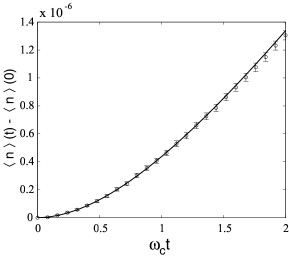
Figure 1: Comparison between analytical (solid line) and scaled simulation results (circles) with the bars of the standard error for the Lindblad-type case. The figure shows the behavior of the expectation value of the quantum number $\langle n\rangle$ as a function of time. The initial state of the system is a coherent state $|\xi=\sqrt{2}\rangle$. For the parameters used here, the scaling reduces the required ensemble size by a factor on the order of $10^{4}$. The simulation here contains $6\times 10^{5}$ realizations.

IV.2 Non-Lindblad-type unravelling in the doubled Hilbert space

For the non-Lindblad-type case we choose the following parameters $2\alpha^{2}kT/\omega_{c}=2.4\times 10^{-6}$, $r=0.1$, $\alpha^{2}\omega_{0}/\omega_{c}=0.5\times 10^{-8}$, and the scaling factor $\beta=10^{5}$. As initial state we choose a superposition of Fock states $\psi=(|0\rangle+|1\rangle)/\sqrt{2}$.

The doubled Hilbert space state vector for the harmonic oscillator reads

$$\theta(t)=\left(\begin{array}[]{c}\phi\left(t\right)\\ \psi\left(t\right)\end{array}\right)=\left(\begin{array}[]{c}\sum_{n=0}^{\infty}\phi_{n}(t)|n\rangle\\ \sum_{n=0}^{\infty}\psi_{n}(t)|n\rangle\\ \end{array}\right),$$ (37)

where $\phi_{n}(t)$ and $\psi_{n}(t)$ are the probability amplitudes in the Fock state basis.

By comparing Eq. (31) with the master equation (1), the operators $A(t)$ and $B(t)$ have to be chosen as

$$A(t) = B(t)=-i\omega_{0}a^{{\dagger}}a-\frac{1}{2}\left\{\left[\Delta(t)+\Gamma(t)\right]a^{{\dagger}}a+\right.$$ (38)

$$\left.\left[\Delta(t)-\Gamma(t)\right]aa^{{\dagger}}\right\}.$$

Accordingly, the operators $C_{i}$ and $D_{i}$ are

$$C_{1}(t) = D_{1}(t)=\sqrt{|\Delta(t)-\Gamma(t)|}a^{{\dagger}},$$

$$C_{2}(t) = D_{2}(t)=\sqrt{|\Delta(t)+\Gamma(t)|}a$$ (39)

and the corresponding operators $J_{i}$, become

$$J_{1}(t)=\sqrt{|\Delta(t)-\Gamma(t)|}\left(\begin{array}[]{cc}{\rm sgn}\left[\Delta(t)-\Gamma(t)\right]a^{{\dagger}}&0\\ 0&a^{{\dagger}}\\ \end{array}\right)$$ (42)

$$J_{2}(t)=\sqrt{|\Delta(t)+\Gamma(t)|}\left(\begin{array}[]{cc}{\rm sgn}\left[\Delta(t)+\Gamma(t)\right]a&0\\ 0&a\\ \end{array}\right).$$ (45)

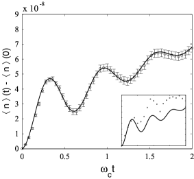
Figure 2: Comparison between analytical (solid line) and scaled simulation results (circles) with the bars of the standard error for the non-Lindblad-type case. The figure shows the behavior of the expectation value of the quantum number $\langle n\rangle$ as a function of time. The initial state of the system is the superposition of Fock states $(|0\rangle+|1\rangle)/\sqrt{2}$. For the parameters used here, the scaling reduces the required ensemble size atleast by a factor of $10^{4}$. The simulation contains $6\times 10^{5}$ realizations. The inset shows (in the same scale as the main plot) the poor match between the analytical result (solid line) and the simulation result without the scaling (circles) with $6\times 10^{8}$ realizations which is three orders of magnitude larger than used in the scaling (see text).

The statistics of the quantum jumps is described by the waiting time distribution function $F_{w}(\tau)$ which represents the probability that the next jump occurs within the time interval $[t,t+\tau)$. $F_{w}(\tau)$, derived from the properties of the stochastic process, reads

$$F_{w}(\tau)=1-\exp\left[-\int_{0}^{\tau}\sum_{i=1,2}P_{i}\left(s\right)ds\right],$$ (46)

where for channel 1 (jump up, the system absorbs a quantum of energy from the environment)

$$P_{1}(t)=\beta~{}\frac{|\Delta(t)-\Gamma(t)|}{\|\theta\left(t\right)\|^{2}}\sum_{n=0}^{\infty}(n+1)\left[|\phi_{n}(t)|^{2}+|\psi_{n}(t)|^{2}\right],$$ (47)

and for channel $2$ (jump down, the system emits a quantum of energy into the environment)

$$P_{2}(t)=\beta~{}\frac{|\Delta(t)+\Gamma(t)|}{\|\theta\left(t\right)\|^{2}}\sum_{n=0}^{\infty}n\left[|\phi_{n}(t)|^{2}+|\psi_{n}(t)|^{2}\right].$$ (48)

Here, the probabilities are scaled with a factor of $\beta$ according to the scaling scheme presented above. When the jump occurs, the choice of the decay channel is made according to the factors $P_{1}(t)$ and $P_{2}(t)$. The times at which the jumps occur are obtained from Eq. (46) by using the method of inversion Breuer02a .

Figure 2 displays the short time oscillatory non-Markovian behavior of the average quantum number $\langle n\rangle$. This type of behavior is studied in detail in Ref. Maniscalco04a . The results show the excellent match between the exact analytical solution and the simulation results using the scaling with $6\times 10^{5}$ realizations. Again, the results confirm the validity of the scaling procedure. Moreover, the inset shows a very poor match between the non-scaled simulations with $6\times 10^{8}$ realizations Piilo05a and justifies the claim that the reduction in the ensemble size is at least on the order of $10^{4}$ when the scaling procedure is used.

The reduction of the ensemble size can be estimated also by calculating the maximum jump probability of a single realization. In the example considered here, the maximum probability is of the order of $10^{-7}$, in other words on average an ensemble size of $10^{7}$ produces one jump event in the unscaled simulations. We estimate that one needs several hundreds jumps in the simulations to produce accurately the rich dynamical features of the heating function displayed in Fig. 2, and consequently the requirement for the ensemble size is at least $10^{9}$ without the scaling. Thus, the reduction in the ensemble size by the scaling method is again found to be at least on the order of $10^{4}$.

It is interesting to compare the various terms in the scaling equation (29) in the non-Lindblad case. Figure 3 shows the four terms of the scaling equation (29). One can notice that two of the terms practically cancel each other and the final result is mostly given by the two terms presented in Figs. 3 (a) and (d).

V Discussion and conclusions

We have demonstrated a scaling method for Monte Carlo wave-function simulations which can reduce the size of the generated ensemble by several orders of magnitude especially for weakly coupled non-Markovian systems. The scaling is based on the notion that once in the simulations the jump probabilities are scaled, and the deterministic evolution given by the non-Hermitian Hamiltonian left untouched, one can obtain the time evolution of the observables of interest from the scaling equation (29).

The scaling has been used in a restricted form, for a specific physical system, in Ref. Maniscalco04a . In that case the initial state of the system was a Fock state. Here, we present a generalized scaling scheme which is able to treat arbitrary initial states of the system and arbitrary Hamiltonians. We emphasize that the scaling method works very well for solving the short time dynamics of non-Markovian, systems, which bear importance e.g. for the decoherence studies for quantum information processing Alicki02a .

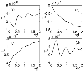
Figure 3: Contribution from the various terms of the scaling equation (29). (a) $T_{A}=\langle A\rangle_{0}(t)$, (b) $T_{B}=-P_{tot}(t)\langle A\rangle_{0}(t)/\beta$, (c) $T_{C}=-[(N-N_{j}(t))/(\beta N)]\langle A\rangle_{0}(t)$, (d) $T_{D}=\langle{\bar{A}}\rangle_{tot}(t)/\beta$. The terms has been shifted to start from the same initial value for easier comparison. Here $A$ is the number operator $A=a^{{\dagger}}a$. The final result presented in Fig. 2. is mostly given as a sum of the terms displayed in (a) and (d).

In general, non-Markovian systems, even when they are weakly coupled to their environments, can posses rich dynamical features despite of the fact that the quantum jump probability per stochastic realization is small during the time evolution period of interest (see the examples above). This is the key area where the scaling method we have presented is useful. The small jump probabilities due to the weak coupling can lead to the situations where the requirement for the size of the generated ensemble in the Monte Carlo wave function simulations is unconveniently large. In these cases, the scaling method can be used to reduce and optimize the generated ensemble size for efficient numerical simulation of weakly coupled non-Markovian systems.

The scaling method presented here can be used when the master equation of the open quantum system can be expressed in the general form of Eq. (1) obtained by the time-convolutionless projection operator techniques (the one-jump restriction still applies, see below). To compare our method to the other simulation methods for non-Markovian systems one should actually compare the validity of the TCL with respect to the methods presented e.g. in Refs. Imamoglu96a ; Yu99a ; Gambetta02a . Thus, making a rigorous comparison is an involved task and is left for future studies. We initially note here that our method is not restricted with respect to the temperature of the environment (while method presented in Ref. Gambetta02a is valid for the zero-temperature bath) and is valid, at least in principle, to the order used in the TCL expansion of master equation to be unravelled (while method presented in Ref. Yu99a is post-Markovian, i.e. first order correction to Markovian dynamics). However, it is worth mentioning that the validity of the TCL expansion is crucially related to the existence of the TCL generator (see e.g. page $447$ of Ref. Breuer02a ).

The scaling method is limited to the cases where there is maximally one jump per realization in the generated Monte Carlo ensemble. Moreover, it is also important to note that the same restriction applies also for the scaled simulations. These limits can be easily checked by calculating the jump probabilities from Eqs. (6) and (46) for the time period of interest or by monitoring the number of jumps in the simulations. As soon as more than one jump per realization in the scaled simulations begin to occur, one can estimate the error by calculating the ratio between the two-jump and the one-jump probabilities per realization. In the examples we have described, we have not used very aggressive optimization of the ensemble size (though the ensemble size reduction is on the order of $10^{4}$), and no error has been introduced. This has been confirmed by monitoring the jumps in the simulations: no two-jump realizations was generated. Thus, the error bars displayed in the Figs. (1) and (2) correspond to the usual statistical error (standard deviation) of the Monte Carlo ensemble.

In conclusion, the scaling method has limitations (one jump per realization) but it is interesting to note that in the region where the method can not be applied (more than one jump per realization), it is not needed. This is because in this region there already occurs large enough number of jumps enhancing the statistical accuracy of the simulations. In other words, the problem which the scaling solves appears only within the region of validity of the method.

Appendix A Hilbert space path integral

Expanding the exponential waiting time distribution $F$ and taking into account the terms corresponding to maximum one jump per realization for short times and weak couplings, the contribution to the propagator from the path without the jumps is Breuer02a

$$T^{(0)}\left[\psi,t|\psi_{0},0\right]=\left(1-F\left[\psi_{0},t\right]\right)\delta\left[\psi-g_{t}\left(\psi_{0}\right)\right]=$$

$$\left(1-\int_{0}^{t}ds\sum_{i}\gamma_{i}(s)\|L_{i}g_{s}(\psi_{0})\|^{2}\right)\times$$

$$\delta\left(\psi-g_{t}\left(\psi_{0}\right)\right)$$ (49)

where $\delta\left(\psi-g_{t}\left(\psi_{0}\right)\right)$ is the functional delta-function and the deterministic evolution according to the non-Hermitian Hamiltonian $H$ is given by

$$g_{t}\left(\psi_{0}\right)=\frac{\exp\left(-i\int_{0}^{t}H(t^{\prime})dt^{\prime}\right)\psi_{0}}{\|\exp\left(-i\int_{0}^{t}H(t^{\prime})dt^{\prime}\right)\psi_{0}\|}.$$ (50)

where

$$H=H_{S}-\frac{\imath\hbar}{2}\sum_{i}\gamma_{i}(t)L_{i}^{{\dagger}}L_{i}.$$ (51)

By using the recursion relation for the propagator $T$ Breuer02a and neglecting the terms of the order of $\gamma_{i}(t)^{2}$ or higher, one can now calculate the contribution of the one jump path to the propagator as

$$T^{(1)}\left[\psi,t|\psi_{0},0\right]=\int_{0}^{t}ds\int D\psi_{1}D\psi_{1}^{*}\int D\psi_{2}D\psi_{2}^{*}~{}$$

$$\delta\left(\psi-g_{t}\left(\psi_{2}\right)\right)\sum_{i}\gamma_{i}(s)\|L_{i}\psi_{1}\|^{2}\delta\left(\frac{L_{i}\psi_{1}}{\|L_{i}\psi_{1}\|}-\psi_{2}\right)$$

$$\delta\left(\psi_{1}-g_{s}\left(\psi_{0}\right)\right).$$ (52)

where the transition rate summed over the decay channels is

$$W\left[\psi_{2}|\psi_{1}\right]=\sum_{i}\gamma_{i}(s)\|L_{i}\psi_{1}\|^{2}\delta\left[\frac{L_{i}\psi_{1}}{\|L_{i}\psi_{1}\|}-\psi_{2}\right],$$ (53)

The physical interpretation of Eq. (52) is straightforward. The integrations sums over the various one jump routes and over all the possible jump times.

Appendix B Expectation value

In the simulations we scale up the jump probabilities by a factor $\beta$, and leave the non-Hermitian Hamiltonian as it is [includes also $\gamma_{i}(t)$], we get the corresponding equation for Eq. (27) as

$$\beta\left[\langle A\rangle\left(t\right)-\langle A\rangle_{0}(t)\right]=\int D\psi D\psi^{*}~{}\langle\psi|A|\psi\rangle$$

$$\times\left\{-\delta\left(\psi-g_{t}(\psi_{0})\right)\int_{0}^{t}ds\sum_{i}\beta\gamma_{i}(s)\|L_{i}g_{s}(\psi)\|^{2}\right.$$

$$+\int_{0}^{t}ds\int D\psi_{1}D\psi_{1}^{*}\int D\psi_{2}D\psi_{2}^{*}~{}\delta\left(\psi-g_{t}(\psi_{2})\right)$$

$$\times\sum_{i}\beta\gamma_{i}(s)\|L_{i}\psi_{1}\|^{2}\delta\left(\frac{L_{i}\psi_{1}}{\|L_{i}\psi_{1}\|}-\psi_{2}\right)$$

$$\times\delta\left(\psi_{1}-g_{s}(\psi_{0})\right)\bigg{\}}.$$ (54)

For scaling to work, we have to be able to extract from the simulations the information on the r.h.s. of this equation.

This can be done as follows. We note the first term on the r.h.s. of Eq. (54) as

$$\bar{\langle A\rangle_{0}}(t)=P_{tot}(t)\langle A\rangle_{0}(t)$$ (55)

where $P_{tot}(t)$ is the total transition rate

$$P_{tot}(t)=\int_{0}^{t}ds\sum_{i}\beta\gamma_{i}(s)\|L_{i}g_{s}(\psi)\|^{2}.$$ (56)

Furthermore, we denote by $\bar{\langle A\rangle_{1}}$ the second term on the r.h.s. of Eq. (54) as

$$\bar{\langle A\rangle_{1}}(t)=\int D\psi D\psi^{*}~{}\langle\psi|A|\psi\rangle$$ (57)

$$\left[\int_{0}^{t}ds\int D\psi_{1}D\psi_{1}^{*}\int D\psi_{2}D\psi_{2}^{*}~{}\delta\left(\psi-g_{t}(\psi_{2})\right)\right.$$

$$\left.\times\sum_{i}\beta\gamma_{i}(s)\|L_{i}\psi_{1}\|^{2}\delta\left(\frac{L_{i}\psi_{1}}{\|L_{i}\psi_{1}\|}-\psi_{2}\right)\delta\left(\psi_{1}-g_{s}(\psi_{0})\right)\right]$$

$$= \frac{N_{j}(t)}{N}\sum_{i=1}^{N_{j}(t)}\langle\psi_{i}(t)|A|\psi_{i}(t)\rangle/N_{j}(t),$$

where $N_{j}(t)$ is number of jumps, and $N$ the total number of realizations. Here, the second part is the one jump contribution to the expectation value, expressed formally, and the summation is carried over those realizations that have jumped till time $t$. The corresponding simulation presentation (simulation average) is given in the last part.

Now the ensemble average of all realizations $\bar{\langle A\rangle}_{tot}(t)$, the quantity which we can easily calculate in the simulation, is given by as a sum of 0 and 1 jump realization contributions

$$\bar{\langle A\rangle}_{tot}(t)=\frac{N-N_{j}(t)}{N}\langle A\rangle_{0}(t)+\bar{\langle A\rangle}_{1}(t).$$ (58)

Equation (54), which includes the quantity we are interested in, can now be written as

$$\beta\left[\langle A\rangle\left(t\right)-\langle A\rangle_{0}(t)\right]=-\bar{\langle A\rangle}_{0}(t)+\bar{\langle A\rangle}_{1}(t)=$$

$$-P_{tot}\langle A\rangle_{0}(t)-\frac{N-N_{j}}{N}\langle A\rangle_{0}(t)+\bar{\langle A\rangle}_{tot}(t).$$ (59)

From this equation we easily obtain the final result for the expectation value of arbitrary operator $A$ in compact form as

$$\langle A\rangle(t) = \left(1-\frac{P_{tot}(t)}{\beta}-\frac{1}{\beta}\frac{N-N_{j}(t)}{N}\right)\langle A\rangle_{0}(t)$$ (60)

$$+\frac{1}{\beta}\bar{\langle A\rangle}_{tot}(t).$$

References

- (1) H.-P. Breuer and F. Petruccione, The Theory of Open Quantum Systems, (Oxford University Press, Oxford, 2002).
- (2) E. Joos, H.-D. Zeh, C. Kiefer, D. Giulini, J. Kupsch, and I.-O. Stamatescu, Decoherence and the Appearance of a Classical World in Quantum Theory, 2nd ed. (Springer-Verlag, Berlin, 2003)
- (3) M. A. Nielsen and I. L. Chuang, Quantum Computation and Quantum Information (Cambridge University Press, Cambridge, England, 2000).
- (4) C. J. Myatt et al., Nature 403, 269 (2000); Q.A. Turchette et al., Phys. Rev. A 62, 053807 (2000).
- (5) J.F. Poyatos, J.I. Cirac, and P. Zoller, Phys. Rev. Lett. 77, 4728 (1996).
- (6) M.B. Plenio and S.F. Huelga, Phys. Rev. Lett. 88, 197901 (2002).
- (7) J. Dalibard, Y. Castin, and K. Mølmer, Phys. Rev. Lett. 68, 580 (1992); K. Mølmer, Y. Castin, and J. Dalibard, J. Opt. Soc. Am. B 10, 524 (1993).
- (8) K. Mølmer and Y. Castin, Quantum Semiclass. Opt. 8, 49 (1996).
- (9) N. Gisin and I. C. Percival, J. Phys. A 25, 5677 (1992); N. Gisin and I. C. Percival, J. Phys. A 26, 2233 (1993); N. Gisin and I. C. Percival, J. Phys. A 26, 2245 (1993).
- (10) W. T. Strunz, L. Diòsi, and N. Gisin, Phys. Rev. Lett. 82, 1801 (1999).
- (11) L. Diòsi, N. Gisin, and W. T. Strunz, Phys. Rev. A 58, 1699 (1998).
- (12) H.-P. Breuer, B. Kappler, and F. Petruccione, Phys. Rev. A 59, 1633 (1999).
- (13) H.-P. Breuer, Phys. Rev. A 70, 012106 (2004).
- (14) Y. Castin and K. Mølmer, Phys. Rev. Lett. 74, 3772 (1995).
- (15) L. Diòsi, N. Gisin, J. Halliwell, and I.C. Percival, Phys. Rev. Lett. 74, 203 (1995).
- (16) S. Maniscalco, J. Piilo, F. Intravaia, F. Petruccione, and A. Messina, Phys. Rev. A 70 032113 (2004).
- (17) S. Maniscalco, J. Piilo, F. Intravaia, F. Petruccione, and A. Messina, Phys. Rev. A 69 052101 (2004).
- (18) H. Carmichael, An Open System Approach to Quantum Optics, Volume m18 of Lecture Notes in Physics (Springer-Verlag, Berlin, 1993)
- (19) C. W. Gardiner and P. Zoller, Quantum Noise: A Handbook of Markovian and non-Markovian Quantum Stochastic Methods with Applications to Quantum Optics (Springer-Verlag, Berlin, 1999).
- (20) M. B. Plenio and P. L. Knight, Rev. Mod. Phys. 70, 101 (1998), and references therein.
- (21) G. Lindblad, Communn. Math. Phys. 48 119 (1976).
- (22) V. Gorini, A. Kossakowski, and E. C. G. Sudarshan, J. Math. Phys. 17, 821 (1976).
- (23) S. Maniscalco, F. Intravaia, J. Piilo and A. Messina, J. Opt. B: Quantum Semiclassical Opt. 6, S98 (2004).
- (24) F. Intravaia, S. Maniscalco, and A. Messina, Eur. Phys. J. D 32 97 (2003).
- (25) A.O. Caldeira and A.J. Leggett, Phys. A 121, 587 (1983).
- (26) F. Intravaia, S. Maniscalco, and A. Messina, Phys. Rev. A 67, 042108 (2003).
- (27) This is the largest ensemble size we can conveniently generate with the current computer resources at our disposal.
- (28) R. Alicki, M. Horodecki, P. Horodecki, and R. Horodecki, Phys. Rev. A 65, 062101 (2002).
- (29) P. Stenius and A. Imamoḡlu, Quantum Semiclassic. Opt. 8, 283 (1996).
- (30) T. Yu, L. Diósi, N. Gisin, and W. T. Strunz, Phys. Rev. A 60, 91 (1999).
- (31) J. Gambetta and H. M. Wiseman, Phys. Rev. A 66, 052105 (2002).