Conditioning two-party quantum teleportation within a three-party quantum channel

Abstract

We consider an arbitrary continuous variable three-party Gaussian quantum state which is used to perform quantum teleportation of a pure Gaussian state between two of the parties (Alice and Bob). In turn, the third party (Charlie) can condition the process by means of local operations and classical communication. We find the best measurement that Charlie can implement on his own mode that preserves the Gaussian character of the three-mode state and optimizes the teleportation fidelity between Alice and Bob.

I Introduction

Quantum information processing with continuous variables (CV) provides an interesting alternative to the traditional qubit-based approach. CV seem to be particularly suitable for quantum communications, as for example quantum teleportation telepo and quantum key distribution QKD . Multipartite CV entangled states for quantum communication networks are rather easy to produce. In particular, tripartite entangled Gaussian states realized either using squeezers and beam splitters Braun , interlinked bilinear interactions parisopto or through radiation pressure PRL ; PRA ; network ; JOBSO have been considered for the realization of a quantum teleportation network and for telecloning. Tripartite CV entanglement between optical modes has been generated using squeezing and beam splitters and experimentally characterized in cinjap , and it has been recently exploited for the realization of quantum secret sharing in Lance and for quantum telecloning in FuruNat . Here we consider a generic CV tripartite Gaussian state which is employed for the specific task of teleporting a pure Gaussian state between two of the three parties (Alice and Bob). We determine the best way the third party (Charlie) can cooperate to improve this teleportation task. To be more specific, we find the optimal Gaussian measurement at Charlie’s site which maximizes the teleportation fidelity. This is different from the optimization over all possible local Gaussian operation of CV teleportation as considered in fiurasek and also from the problem of entanglement distillation distill , where one always starts from bipartite entangled states and tries to increase their entanglement. In Sec. II we present the scenario and describe the teleportation protocols in the case when it is assisted or is not assisted by measurements at Charlie’s site. In Sec. III we discuss the case when Charlie performs a dichotomic measurement with a Gaussian and a non-Gaussian outcome, while in Sec. IV we consider the case of a local Gaussian measurement performed at Charlie’s site. In Sec. V various applications of the theorems derived in Sec. III and IV are discussed in detail, while Sec. VI is for concluding remarks.

II Assisted and non-assisted teleportation protocols

The scheme we are going to study is described in Fig. 1: Alice, Bob and Charlie each possess a continuous variable mode, characterized by an annihilation operator $\hat{a},\hat{b}$ and $\hat{c}$ respectively, and share a quantum channel given by an arbitrary three-mode Gaussian state $\rho$, characterized by a displacement $\vec{d}\in{\mathbb{R}}^{6}$ and a correlation matrix (CM)

$$V\equiv\left(\begin{array}[c]{ccc}A&F&E\\ F^{T}&B&D\\ E^{T}&D^{T}&C\end{array}\right),$$ (1)

where the blocks $A,B,...,F$ are $2\times 2$ real matrices. Alice has to teleport to Bob an unknown pure Gaussian state $\rho_{in}$ with CM $V_{in}$ and amplitude $\mu$. The most straightforward strategy is to ignore Charlie (non-assisted protocol) and use the reduced bipartite Gaussian state $\rho^{tr}\equiv{\rm Tr}_{c}(\rho)$ to implement a standard continuous variable teleportation protocol telepo . In such a case, Alice mixes her part of the reduced state $\rho^{tr}$ with the input state $\rho_{in}$ through a balanced beam-splitter and makes a homodyne detection of the output modes, i.e., she measures the quadratures $\hat{X}_{-}\equiv 2^{-1/2}(\hat{X}_{a}-\hat{X}_{in})$ and $\hat{P}_{+}\equiv 2^{-1/2}(\hat{P}_{a}+\hat{P}_{in})$. After the measurement, Alice classically communicates the result $\gamma\equiv-X_{-}+iP_{+}$ to Bob, who performs a conditional displacement $\hat{D}_{b}(\gamma^{\prime})\equiv\exp(\gamma^{\prime}\hat{b}^{\dagger}-\gamma^{\prime\ast}\hat{b})$ on his own mode $b$, where $\gamma^{\prime}=\gamma+\delta$ has the double effect to compensate the displacement due to Alice’s measurement (by $\gamma$) and the displacement of the reduced state (by $\delta$ which is connected with $\vec{d}$, see network ). This means that Bob can always implement (through a suitable displacement $\gamma^{\prime}$) a displacement-independent teleportation protocol, whose fidelity only depends on the CMs of the reduced state and the input state. When Charlie is traced out, $\rho^{tr}$ has the CM

$$V^{tr}=\left(\begin{array}[c]{cc}A&F\\ F^{T}&B\end{array}\right)$$ (2)

and the teleportation fidelity is given by $F^{tr}=(\det\Gamma^{tr})^{-1/2}$ fiurasek , where

$$\Gamma^{tr}\equiv 2V_{in}+RAR+B-RF-F^{T}R$$ (3)

and $R={\rm diag}\left(1,-1\right)$.

An alternative strategy for Alice and Bob is to ask for the help of Charlie (assisted protocol), who can perform a suitable measurement on his own mode $c$ and classically communicate the result to Bob (see Fig. 1). In this modified protocol, Bob performs his displacement only after receiving the information about the measurement outcomes from both Alice and Charlie. For every Charlie’s outcome $n$ (with probability $P_{n}$), Bob can choose a conditional displacement $\gamma_{n}^{\prime}$ aiming at optimizing the conditional fidelity $F^{(n)}$ and therefore the effective fidelity $F=\sum_{n}P_{n}F^{(n)}$ of the protocol conditional . In particular, if the bipartite reduced state conditioned to the outcome $n$, $\rho^{(n)}$, is a Gaussian state, then Bob’s displacement is given by $\gamma_{n}^{\prime}=\gamma+\delta_{n}$ where $\delta_{n}$ exactly cancels the displacement of $\rho^{(n)}$, and therefore the conditional fidelity $F^{(n)}$ depends, as before, only on the CMs. In the following we consider two general kinds of measurement at Charlie’s site: a local dichotomic measurement, with a Gaussian outcome and a non-Gaussian one, and a local Gaussian measurement, defined as a local measurement preserving the Gaussian character of the shared state for every outcome. Our aim is to compare the assisted fidelity $F$ and the non-assisted fidelity $F^{tr}$ for both kinds of measurement. We anticipate that for the dichotomic measurement one does not have an improvement ($F\leq F^{tr}$), but the results achieved for the conditional fidelities $F^{(n)}$ are interesting and they can be directly extended to the case of the Gaussian measurement where one can optimize $F$ and then surely state that $F\geq F^{tr}$.

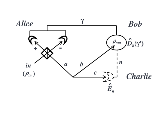
Figure 1: An arbitrary 3-mode Gaussian state is shared by Alice, Bob and Charlie. Alice is supplied with an unknown pure Gaussian state $\rho_{in}$ which she wants to teleport to Bob. In a first strategy, Charlie is traced out and Alice and Bob implement a standard continuous variable teleportation protocol. In an alternative strategy (dashed detector), Bob is helped by Charlie who measures his mode and classically communicates the result $n$ to Bob, who uses also this information for his local operation. Here we consider, for Charlie’s measurement, first a local dichotomic measurement and then a local Gaussian measurement.

III Dichotomic measurement

We first consider the case of a dichotomic measurement with measurement operators $\hat{E}_{0},\hat{E}_{1}\equiv(\hat{I}-\hat{E}_{0}^{2})^{1/2}$ where $\hat{E}_{0}$ is an arbitrary Gaussian state with displacement $\vec{d}_{0}$ and CM $V_{0}$. This implies that for the outcome $n=0$ the conditional bipartite state $\rho^{(0)}\equiv P_{0}^{-1}{\rm Tr}_{c}(\hat{E}_{0}\rho\hat{E}_{0}^{\dagger})$ is still Gaussian, while for the other outcome it is not Gaussian. One can prove (see Appendix A) that the CM of the reduced state $\rho^{(0)}$ is

$$V^{(0)}=V^{tr}-\left(\begin{array}[c]{cc}EME^{T}&EMD^{T}\\ DME^{T}&DMD^{T}\end{array}\right)$$ (4)

where $M$ is the following 2$\times$2 “measurement matrix”

$$M\equiv\frac{1}{g}\Omega\left[2(\det V_{0}+1/4)V_{0}+4(\det V_{0})C\right]\Omega^{T}$$ (5)

with

$$g\equiv 4\det V_{0}\det C+2(\det V_{0}+1/4){\rm Tr}(V_{0}\Omega C\Omega^{T})+(\det V_{0}+1/4)^{2}>0$$ (6)

and

$$\Omega\equiv\left(\begin{array}[c]{cc}0&-1\\ 1&0\end{array}\right).$$ (7)

If we use Eq. (4) in the right hand side of Eq. (3) instead of Eq. (2), we obtain

$$\Gamma^{(0)}=\Gamma^{tr}-\Sigma^{T}M\Sigma$$ (8)

where

$$\Sigma\equiv E^{T}R-D^{T}.$$ (9)

Now, the conditional teleportation fidelity is given by $F^{(0)}=(\det\Gamma^{(0)})^{-1/2}$ and satisfies the following

Proposition 1

The conditional fidelities $F^{(n)}$ corresponding to the outcomes $n=0,1$ and the assisted fidelity $F$ satisfy the inequality

$$F^{(1)}\leq F\leq F^{tr}\leq F^{(0)}$$ (10)

Proof. The proof of $F^{tr}\leq F^{(0)}$ is based on Eq. (8). Matrix $M$ is real, symmetric and strictly positive and, since $\Sigma$ is real, the matrix $\Sigma^{T}M\Sigma$ is real, symmetric and positive. Likewise $\Gamma^{tr}$ and $\Gamma^{(0)}$ are real, symmetric and strictly positive, and from linear algebra it follows that $\det(\Gamma^{(0)})=\det(\Gamma^{tr}-\Sigma^{T}M\Sigma)\leq\det(\Gamma^{tr})$. The proof of $F^{(1)}\leq F^{tr}$ is a consequence of the previous result. The characteristic functions $\Phi^{tr}$, $\Phi^{(0)}$ and $\Phi^{(1)}$ of states $\rho^{tr}$, $\rho^{(0)}$ and $\rho^{(1)}$ are related by $\Phi^{(1)}=P_{1}^{-1}[\Phi^{tr}-P_{0}\Phi^{(0)}]$ which also shows that $\rho^{(1)}$ is not Gaussian. On the other hand, the fidelity $F^{(1)}$ can be expressed in the form network  $F^{(1)}=\pi^{-1}\int d^{2}\lambda\left|\Phi_{in}(\lambda)\right|^{2}[\Phi^{(1)}(\lambda^{\ast},\lambda)]^{\ast}\exp(-\lambda\delta^{(1)\ast}+\lambda^{\ast}\delta^{(1)})$ where $\Phi_{in}$ is the characteristic function of the input state and $\delta^{(1)}$ is an additional shift optimizing $F^{(1)}$. Now, it is easy to prove that, for every $\delta^{(1)}$, one has $F^{(1)}\leq P_{1}^{-1}[F^{tr}-P_{0}F^{(0)}]\leq P_{1}^{-1}[F^{tr}-P_{0}F^{tr}]=F^{tr}$. Finally, the effective fidelity is given by $F=P_{0}F^{(0)}+P_{1}F^{(1)}$ and, since $F^{(0)}\geq F^{(1)}$, one has $F\geq F^{(1)}$. On the other hand, from inequality $F^{(1)}\leq P_{1}^{-1}[F^{tr}-P_{0}F^{(0)}]$ one can derive $F\leq P_{0}F^{(0)}+[F^{tr}-P_{0}F^{(0)}]=F^{tr}$.   

Eq. (10) shows that the dichotomic measurement leads, on average, to an assisted fidelity $F$ which does not outperform $F^{tr}$, proving that the present dichotomic scheme does not seem to bring advantages in a real teleportation network. However the situation is very interesting from the point of view of the conditional teleportation fidelities $F^{(n)}$. In fact Eq. (10) shows that teleportation fidelity always increases if Charlie performs a measurement and the corresponding conditional state is still Gaussian ($F^{(0)}\geq F^{tr}$), while it always decreases with respect to the trace case for the outcome corresponding to the non-Gaussian conditional state ($F^{(1)}\leq F^{tr}$), even if in this latter case the conditional bipartite state is more pure than that without measurement Chuang . This result suggests which is the right kind of measurement to be considered at Charlie’s site (local Gaussian measurement) and it will be the starting point of the next section IV.

Moreover, the dichotomic scheme can be used in a probabilistic way, i.e., selecting only the Gaussian outcome. In this case Bob asks Alice to perform the Bell measurement and the classical communication only if Charlie’s measurement has given the Gaussian outcome. In such a case the assisted fidelity $F$ is just the conditional one $F^{(0)}$, but the protocol has a success probability equal to $P_{0}$.

We have also explicitly verified (see section V.B) that the Gaussian outcome $n=0$ can give $F^{(0)}>1/2$ for the teleportation of coherent states when $\rho^{tr}$ is not entangled (and therefore $F^{tr}\leq 1/2$). In other words, Charlie can conditionally generate remote bipartite entanglement between Alice and Bob if the dichotomic measurement selects the Gaussian outcome. All these considerations make clear why it is profitable to optimize the “Gaussian” conditional fidelity $F^{(0)}$ upon the measurement parameters and exactly such optimization work concerns the remainder of this section.

Thus we restrict to the Gaussian outcome ($n=0$), and look for the optimal Gaussian state $\hat{E}_{0}$ (i.e. the optimal CM $V_{0}$) which maximizes the fidelity $F^{(0)}$. As a first result we can prove the following

Proposition 2

For every Gaussian state $\hat{E}_{0}$, there exists a pure Gaussian state $\hat{E}_{0,p}$ such that $F^{(0,p)}\geq F^{(0)}$.

Proof. For every Gaussian state $\hat{E}_{0}$, there exists a Gaussian unitary transformation $\hat{U}$ such that $\hat{E}_{0}=\hat{U}\rho(n_{T})\hat{U}^{\dagger}$ where $\rho(n_{T})$ is a thermal state with $n_{T}\geq 0$ mean number of photons duan . Thus, we can rewrite the reduced state $\rho^{(0)}\equiv P_{0}^{-1}{\rm Tr}_{c}(\hat{E}_{0}\rho\hat{E}_{0}^{\dagger})=P_{0}^{-1}{\rm Tr}_{c}[\rho(n_{T})\hat{U}^{\dagger}\rho\hat{U}\rho(n_{T})]$ so that the fidelity $F^{(0)}$ achieved from the tripartite Gaussian state $\rho$ and the measurement operator $\hat{E}_{0}$ is the same which is achieved from the tripartite Gaussian state $\hat{U}^{\dagger}\rho\hat{U}$ and the measurement operator $\rho(n_{T})$ i.e. $F^{(0)}\equiv F(\rho,\hat{E}_{0})=F[\hat{U}^{\dagger}\rho\hat{U},\rho(n_{T})]$. On the other hand, denoting with $M(n_{T})$ the measurement matrix corresponding to a thermal state $\rho(n_{T})$, it is easy to prove that $M(0)-M(n_{T})\geq 0$ $\forall n_{T}\geq 0$. From this relation and Eq. (8), one has that $F[\hat{U}^{\dagger}\rho\hat{U},\rho(n_{T})]\leq F[\hat{U}^{\dagger}\rho\hat{U},\rho(0)]$, but $F^{(0)}=F[\hat{U}^{\dagger}\rho\hat{U},\rho(n_{T})]\leq F[\hat{U}^{\dagger}\rho\hat{U},\rho(0)]=F[\rho,\hat{U}\rho(0)\hat{U}^{\dagger}]$ with $\hat{U}\rho(0)\hat{U}^{\dagger}\equiv\hat{E}_{0,p}$ pure Gaussian state.   

According to this latter result, the optimal Gaussian measurement operator $\hat{E}_{0}$ is actually a projection onto a pure Gaussian state and therefore has to be searched within the set of squeezed states $\left|\alpha,\varepsilon\right\rangle=\hat{D}(\alpha)\hat{S}(\varepsilon)\left|0\right\rangle$. Here $\hat{D}(\alpha)$ is the displacement operator with $\alpha$ complex amplitude, while $\hat{S}(\varepsilon)$ is the squeezing operator with $\varepsilon\equiv r\exp(2i\varphi)$ and $r,\varphi$ are the squeezing factor and phase respectively milburn . Since the CM of the input state, $V_{in}$, is given, Charlie has to optimize the protocol only with respect to the CM $V_{0}$ of the squeezed state $\left|\alpha,\varepsilon\right\rangle$, which is given by

$$V_{0}(\xi,\varphi)=\frac{1}{2}\left(\begin{array}[c]{cc}\xi\sin^{2}\varphi+\xi^{-1}\cos^{2}\varphi&(\xi-\xi^{-1})\cos\varphi\sin\varphi\\ (\xi-\xi^{-1})\cos\varphi\sin\varphi&\xi\cos^{2}\varphi+\xi^{-1}\sin^{2}\varphi\end{array}\right)$$ (11)

where $\xi\equiv\exp(2r)$, and therefore the optimization has to be done with respect to $\xi$ and $\varphi$. Finding a global maximum point $(\bar{\xi},\bar{\varphi})$ is difficult in general and therefore we split the problem in two steps: we first maximize the fidelity $F^{(0,p)}\equiv F(\xi,\varphi)$ with respect to $\xi$ for an arbitrary but fixed $\varphi$, and then we maximize the result $F(\bar{\xi}(\varphi),\varphi)$ with respect to $\varphi$. Mathematically speaking the function $F(\xi,\varphi)$ is bounded and continuous in the domain $]0,+\infty[\times[0,\pi]$ and we implicitly have to consider its continuous extension in $[0,+\infty]\times[0,\pi]$ in order to surely have the existence of global extremal points. The first step of maximization is solved by the following

Proposition 3

For every squeezing phase $\varphi\in[0,\pi]$, Charlie can select a squeezing factor $\bar{\xi}(\varphi)$ such that $F(\bar{\xi}(\varphi),\varphi)\geq F(\xi,\varphi)$ $\forall\xi$ (phase-dependent global maximum point). The point $\bar{\xi}(\varphi)$ can be derived analytically from the CMs $V$ and $V_{in}$, according to the following four-step procedure:

1. Construct the matrices $\Gamma^{tr}$ of Eq. (3), $\Sigma$ of Eq. (9) and $U\equiv\Sigma\Omega\Gamma^{tr}\Omega^{T}\Sigma^{T}$.

2. Define a 2-D vector

   $$\vec{u}\equiv\left(\begin{array}[c]{c}\det C+1/4\\ (\det\Sigma)^{2}-{\rm Tr}(\Omega C\Omega^{T}U)\end{array}\right)$$ (12)

   and a 2-D phase-dependent vector

   $$\vec{k}(\varphi)\equiv\left(\begin{array}[c]{c}\vec{\varphi}^{T}U\vec{\varphi}\\ \vec{\varphi}^{T}C\vec{\varphi}\end{array}\right)$$ (13)

   where $\vec{\varphi}^{T}\equiv(\sin\varphi,\cos\varphi)$.

3. Define the scalar product

   $$\gamma(\varphi)\equiv\vec{u}\cdot\vec{k}(\varphi)$$ (14)

   and the third component of the vector product

   $$\omega(\varphi)\equiv\frac{1}{2}[\vec{k}(\varphi)\times\vec{k}(\varphi-\pi/2)]_{z}.$$ (15)

4. Denote with $p(\varphi)$ the $\varphi$-dependent logic proposition $\gamma(\varphi)<0\wedge\gamma(\varphi-\pi/2)<0$.

Then:

$$p(\varphi) =1\Longleftrightarrow\bar{\xi}(\varphi)=\frac{\omega(\varphi)-\sqrt{\omega(\varphi)^{2}+\gamma(\varphi-\pi/2)\gamma(\varphi)}}{\gamma(\varphi-\pi/2)}\equiv\xi_{-}(\varphi)$$ (16)

$$p(\varphi) =0\Longleftrightarrow\bar{\xi}(\varphi)=0\text{\quad}\vee\quad\bar{\xi}(\varphi)=+\infty.$$ (17)

See Appendix B for the proof.

The second step concerns the maximization over the squeezing phase $\varphi$. Using vectors $\vec{u}^{T}=(u_{x},u_{y})$ in (12) and $\vec{k}(\varphi)^{T}=(k_{x}(\varphi),k_{y}(\varphi))$ in (13), the fidelity can be written as

$$F(\xi,\varphi)=\left[\det\Gamma^{tr}-\frac{-u_{y}+(\xi/2)k_{x}(\varphi-\pi/2)+(\xi^{-1}/2)k_{x}(\varphi)}{u_{x}+(\xi/2)k_{y}(\varphi-\pi/2)+(\xi^{-1}/2)k_{y}(\varphi)}\right]^{-1/2}.$$ (18)

We then consider the piecewise continuous function of $\varphi$, $\xi=\bar{\xi}(\varphi)$ defined according to (16), (17) and the corresponding phase-dependent teleportation fidelity $\bar{F}(\varphi)\equiv F(\bar{\xi}(\varphi),\varphi)$ which is continuous on $[0,\pi]$. From Eq. (11) one has

$$V_{0}(\xi,\varphi)=V_{0}(\xi,\varphi+\pi)=V_{0}(\xi^{-1},\varphi+\pi/2)$$ (19)

and therefore $F(0,\varphi)=F(+\infty,\varphi+\pi/2)$ and $F(0,\varphi+\pi/2)=F(+\infty,\varphi)$. This implies that finding the maximum point $\bar{\varphi}$ of $\bar{F}(\varphi)$ is equivalent to find the maximum point of the piecewise continuous function

$$\tilde{F}(\varphi)=\left\{\begin{array}[c]{c}F(\xi_{-}(\varphi),\varphi)\qquad\quad\qquad\qquad\qquad\qquad\qquad\mathrm{if}\quad p(\varphi)=1\\ F(0,\varphi)=[\det\Gamma^{tr}-k_{x}(\varphi)/k_{y}(\varphi)]^{-1/2}\qquad\mathrm{if}\quad p(\varphi)=0\quad.\end{array}\right.$$ (20)

Now, one has three cases: i) $\bar{\varphi}$ is a stationary point of $F(0,\varphi)$; ii) $\bar{\varphi}$ is a stationary point of $F(\xi_{-}(\varphi),\varphi)$; iii) $\bar{\varphi}$ is one of the border points dividing the intervals where $p(\varphi)=1$ from those where $p(\varphi)=0$. We report a simple analytical expression of the final global maximum point only in the first case, while in the other two cases the expressions are extremely involved. In case i), defining the $2\times 2$ matrix $\tau\equiv U\Omega C\Omega^{T}$, the stationary points $\varphi_{\pm}$ of $F(0,\varphi)$ are given by the relation

$$\cos 2\varphi_{\pm}=\frac{\tau_{12}^{2}-\tau_{21}^{2}\pm(\tau_{11}-\tau_{22})\sqrt{(\tau_{11}-\tau_{22})^{2}+4\tau_{12}\tau_{21}}}{(\tau_{11}-\tau_{22})^{2}+(\tau_{12}+\tau_{21})^{2}}.$$ (21)

In many cases of practical interest (for instance when coherent states or $\varphi=0$ squeezed states are teleported through a CM $V$ with diagonal blocks, as for example in Braun ; PRL ; PRA ; parisopto ), the above procedure allows to find the maximum point $(\bar{\xi}(\bar{\varphi}),\bar{\varphi})$ and the corresponding optimal conditional fidelity $F^{(0)}_{max}=F(\bar{\xi}(\bar{\varphi}),\bar{\varphi})$ quite quickly. In some easy cases when matrices $U$ and $C$ are proportional to the identity, we see from (13) that the above optimization becomes $\varphi$-independent and therefore the maximum point is given by $\bar{\xi}=1$ if $\gamma<0$ or by $\bar{\xi}=0$ if $\gamma\geq 0$. In the first case the optimal Gaussian state is a coherent state, i.e. $\hat{E}_{0}^{opt}=\left|\alpha\right\rangle\left\langle\alpha\right|$ (with $\alpha$ arbitrary), while in the second case it is an infinitely squeezed state, i.e. $\hat{E}_{0}^{opt}=\left|X(\varphi)\right\rangle\left\langle X(\varphi)\right|$ where $\hat{X}(\varphi)\equiv 2^{-1/2}(\hat{c}\,e^{-i\varphi}+\hat{c}^{\dagger}\,e^{i\varphi})$ (phase $\varphi$ and eigenvalue $X(\varphi)$ are arbitrary).

IV Local Gaussian measurement

The above optimization results (propositions 2 and 3) refer to the conditional scheme where Charlie performs a dichotomic measurement and the Gaussian outcome $n=0$ is selected, and they can be directly used for the conditional generation of entanglement in that configuration. However, these results can be extended to a different scheme where all the measurement outcomes are Gaussian and therefore all the conditional fidelities can potentially outperform $F^{tr}$ according to Proposition 1. More in detail, Proposition 1 suggests to consider for Charlie a measurement which creates a conditional bipartite state which is Gaussian for every outcome, and we surely achieve this condition if we consider for Charlie a local Gaussian measurement, i. e., a local measurement $\{\hat{E}(n)\}$ transforming a Gaussian multipartite state into another Gaussian state for every measurement outcome $n$. Notice that here we include in the Gaussian states also asymptotic Gaussian states, such as the infinitely squeezed states. Examples of local Gaussian measurements are provided by heterodyne measurement on a single mode $c$, i.e., $\{|\alpha\rangle\langle\alpha|/\sqrt{\pi},\alpha\in\mathbb{C}\}$, or they are obtained when the $c$ mode is coupled to ancillary modes by a Gaussian unitary interaction and then the ancillas are subject to heterodyne or homodyne measurement. Consider then an assisted protocol where Charlie performs a local Gaussian measurement $\{\hat{E}(n)\}$ on his mode $c$ and classically communicates the measurement result $n$ to Bob (who, in turn, makes a drift-cancelling displacement depending upon the measurement outcomes of both Alice and Charlie). It is possible to prove a result analogous to Proposition 2 of the dichotomic case:

Proposition 4

For every local Gaussian measurement $\{\hat{E}(n)\}$ with fidelity $F$, there exists a “pure” local Gaussian measurement $\{\hat{E}_{\varepsilon}(\alpha)\equiv\left|\alpha,\varepsilon\right\rangle\left\langle\alpha,\varepsilon\right|/\sqrt{\pi},\alpha\in\mathbb{C}\}$ with a suitable $\varepsilon$, such that its fidelity $F(\varepsilon)\geq F$.

Proof. Suppose that Charlie performs an arbitrary local Gaussian measurement $\{\hat{E}(n)\}$ on his mode $c$, so that the conditional reduced state of Alice and Bob is given by $\rho^{(n)}=P(n)^{-1}\mathrm{Tr}_{c}(\hat{E}(n)\rho\hat{E}(n)^{\dagger})$ corresponding to a fidelity $F^{(n)}$ (the effective fidelity of the protocol is the average over the results $F=\sum_{n}P(n)F^{(n)}$). Suppose now that Charlie performs a further local measurement on $c$ given by a dichotomic measurement and the Gaussian outcome $\hat{E}_{0}$ has been selected. In such a case the reduced state will be $\rho^{(n)\prime}\propto\mathrm{Tr}_{c}(\hat{E}_{0}\hat{E}(n)\rho\hat{E}(n)^{\dagger}\hat{E}_{0}^{\dagger})=\mathrm{Tr}_{c}(\hat{E}(n)^{\dagger}\hat{E}_{0}^{2}\hat{E}(n)\rho)=\mathrm{Tr}_{c}(\hat{E}(n)^{\prime}\rho\hat{E}(n)^{\prime\dagger})$ where $\hat{E}(n)^{\prime}\equiv[\hat{E}(n)^{\dagger}\hat{E}_{0}^{2}\hat{E}(n)]^{1/2}$ is a Gaussian state distill , and the corresponding fidelity will be $F^{(n)\prime}$. From Eq. (10) we have $F^{(n)}\leq F^{(n)\prime}$ $\forall n$, implying $F\leq\sum_{n}P(n)F^{(n)\prime}\leq F^{(\tilde{n})\prime}$ where $F^{(\tilde{n})\prime}$ is the maximum value achieved for a particular outcome $\tilde{n}$. Now, Proposition 2 tells us that there exists a pure Gaussian state $\hat{E}_{p}\equiv\left|\alpha,\varepsilon\right\rangle\left\langle\alpha,\varepsilon\right|$ such that $F^{(p)}\geq F^{(\tilde{n})\prime}$, with a suitably chosen squeezing complex factor $\varepsilon$, while $\alpha$ can be arbitrary. It is then evident that one has a teleportation fidelity $F^{(p)}$ also if Charlie directly applies the measurement $\hat{E}_{\varepsilon}(\alpha)\equiv\left|\alpha,\varepsilon\right\rangle\left\langle\alpha,\varepsilon\right|/\sqrt{\pi}$ on the tripartite state $\rho$ and classically communicates the result $\alpha$ to Bob, so that one has $F(\varepsilon)=F^{(p)}\geq F^{(\tilde{n})\prime}\geq F$.   

Trivially the previous proposition assures the existence of a local Gaussian measurement of the pure form $\{\hat{E}_{\varepsilon}(\alpha)\equiv\left|\alpha,\varepsilon\right\rangle\left\langle\alpha,\varepsilon\right|/\sqrt{\pi},\alpha\in\mathbb{C}\}$ which leads to an assisted fidelity $F(\varepsilon)\geq F^{tr}$. In fact it is sufficient to consider $\{\hat{E}(n)\}=I$ and apply the proposition. More importantly it implies that the optimal local Gaussian measurement must be searched for within the set of pure measurements $\{\{\hat{E}_{\varepsilon}(\alpha)\},\varepsilon\in\mathbb{C}\}$, which is equivalent to maximize with respect to the $2\times 2$ CM $V_{0}(\varepsilon)=V_{0}(\xi,\varphi)$ of Eq. (11). Thanks to this result, the optimization procedure is exactly the one given for the dichotomic measurement, i.e., it is given by the maximization over the squeezing factor as in Proposition 3 and by the subsequent maximization over the squeezing phase. Repeating such procedure it is possible to find an optimal pair of parameters $(\bar{\xi}(\bar{\varphi}),\bar{\varphi})$ which describes the optimal local Gaussian measurement $\{\hat{E}_{\bar{\varepsilon}}(\alpha)\}$ and provides the corresponding optimal assisted fidelity $F(\bar{\xi},\bar{\varphi})$ using (18). Notice that for finite squeezing ($\bar{\xi}\neq 0,+\infty$) the measurement $\{\hat{E}_{\bar{\varepsilon}}(\alpha)\}$ can be realized by first applying a unitary squeezing transformation $\hat{S}(\bar{\varepsilon})$ to mode $c$ and then making heterodyne detection. For infinite squeezing ($\bar{\xi}=0,+\infty$) the measurement $\{\hat{E}_{\bar{\varepsilon}}(\alpha)\}$ is instead equivalent to a homodyne detection, i.e., to $\left|X(\bar{\varphi})\right\rangle_{c}\left\langle X(\bar{\varphi})\right|$ for $\bar{\xi}=+\infty$ and to $\left|X(\bar{\varphi}+\pi/2)\right\rangle_{c}\left\langle X(\bar{\varphi}+\pi/2)\right|$ for $\bar{\xi}=0$, where $\hat{X}(\varphi)\equiv 2^{-1/2}(\hat{c}\,e^{-i\varphi}+\hat{c}^{\dagger}\,e^{i\varphi})$. As for the dichotomic case, we can use this optimized measurement to create conditional bipartite entanglement between Alice and Bob and now this can be done in a deterministic way since all the outcomes are Gaussian. Note that this is not in contrast with the impossibility of entanglement distillation of Gaussian states with local Gaussian operations and classical communications distill because here we only have a transfer of entanglement resources from a tripartite to a bipartite state. In the following section we give explicit examples of application of our optimization procedure.

V Examples

V.1 Optimization of fidelity

As an example of application of our theoretical results, we consider a three-mode Gaussian state with CM

$$V=\left(\begin{array}[c]{ccc}qI&wR&wR\\ wR&sI&tI\\ wR&tI&sI\end{array}\right)$$ (22)

where $R={\rm diag}\left(1,-1\right)$, $I$ is the $2\times 2$ matrix identity, and the coefficients $q,s,t$ and$\ w$ are real numbers. The CM (22) represents a genuine CM (i.e. it corresponds to a physical state) if and only if Cirac3modes

$$V-\frac{i}{2}J\geq 0$$ (23)

where

$$J\equiv\left(\begin{array}[c]{ccc}\Omega&&\\ &\Omega&\\ &&\Omega\end{array}\right)$$ (24)

with $\Omega$ given in (7). Setting $s=(q+1)/2,$ $t=q/2$ and $w=[\sqrt{(2q-1)(q+1)}]/2$ in (22), we have a $q-$dependent CM $V(q)$ which is genuine for every $q\geq 1/2$. This is exactly the correlation matrix considered in game , where a novel (cooperative) telecloning protocol is proved to outperform the standard (non cooperative) one for increasing values of $q$. We call $q$ the ‘noise parameter’ since it determines the linear entropy of the bipartite reduced state $\rho_{tr}\equiv Tr_{c}(\rho)$ used by Alice and Bob in the non-assisted protocol, i.e., $S(\rho_{tr})=1-Tr_{ab}(\rho_{tr}^{2})=q/(q+1)$.

Suppose that Alice, Bob and Charlie possess modes ${\hat{a}}$, $\hat{b}$ and ${\hat{c}}$ respectively, and Alice wants to teleport a coherent state ($V_{in}=I/2$) to Bob with the help of Charlie. Due to the simple form of $V$ and $V_{in}$, it is straightforward to compute the optimal local Gaussian measurement which Charlie can perform in order to optimize teleportation fidelity. From Proposition 4 we know that it has the pure form $\{\left|\alpha,\varepsilon\right\rangle\left\langle\alpha,\varepsilon\right|/\sqrt{\pi},\alpha\in\mathbb{C}\}$ and applying Proposition 3 we can calculate the value $\bar{\varepsilon}\equiv(\bar{\xi},\bar{\varphi})$ corresponding to a maximum. The procedure of Proposition 3 goes as follows:

1. $\Gamma^{tr}=hI$  with $\ h\equiv(1+q+s-2w),$

   $\Sigma=(w-t)I,$

   $U=(w-t)^{2}hI.$

2. $\vec{u}=\left(\begin{array}[c]{c}s^{2}+1/4\\ (w-t)^{2}[(w-t)^{2}-2sh]\end{array}\right),$

   $\vec{k}(\varphi)=\left(\begin{array}[c]{c}(w-t)^{2}h\\ s\end{array}\right)\equiv\vec{k}.$

   Note that, since Charlie’s submatrix $sI$ and matrix $U$ are proportional to the identity, vector $\vec{k}(\varphi)$ becomes $\varphi-$independent and therefore all the subsequent optimization procedure becomes $\varphi-$independent.

3. $\gamma=(w-t)^{2}[s(w-t)^{2}-s^{2}h+h/4],$

   $\omega=0.$

4. As already pointed out at the end of section III, we have the following simplification for Charlie’s optimal measurement

   $$\gamma <0\Longleftrightarrow\bar{\xi}=1$$ (25)

   $$\gamma \geq 0\Longleftrightarrow\bar{\xi}=0.$$ (26)

   The first case corresponds to an heterodyne detection while the second case corresponds to an homodyne detection.

We have $\gamma<0$ for every $q\geq 1/2$ (see Fig. 2) and therefore heterodyne detection ($\bar{\xi}=1$, $\bar{\varphi}$ arbitrary) is the optimal local Gaussian measurement which Charlie can perform in order to maximize teleportation fidelity of coherent states between Alice and Bob with this kind of shared channel. The corresponding optimal assisted fidelity $F(\bar{\xi},\bar{\varphi})$ is computed from (18) setting $\bar{\xi}=1$ and $\bar{\varphi}$ arbitrary, and it is given by

$$F=\{h^{2}-(w-t)^{2}(s+1/2)^{-2}[(2s+1)h-(w-t)^{2}]\}^{-1/2}$$ (27)

which is a function of the noise parameter $q$. Fig. 3 clearly shows the improvement provided by the optimal assisted fidelity $F(q)$ with respect to the non-assisted fidelity $F^{tr}(q)=h^{-1}$ for every $q$ and especially for increasing noise in the channel.

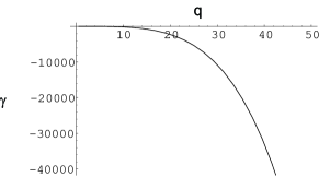
Figure 2: $\varphi$-independent scalar product $\gamma$ versus the noise parameter $q$ for $1/2\leq q\leq 50$.

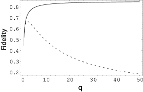
Figure 3: Optimal assisted fidelity $F(q)$ (solid line) and non-assisted fidelity $F^{tr}(q)$ (dashed line) versus the noise parameter $q$ for $1/2\leq q\leq 50$.

V.2 Conditional generation of entanglement

Consider now a three-mode Gaussian state $\rho$ with CM

$$V=\left(\begin{array}[c]{ccc}aI&fI&eR\\ fI&bI&dR\\ eR&dR&cI\end{array}\right)$$ (28)

where $R={\rm diag}\left(1,-1\right)$, $I$ is the $2\times 2$ matrix identity and

$$\{a,b,c,d,e,f\}=\{10.15,5.52,15.2,8.87,12.3,6.96\}.$$ (29)

Numerical values in (29) are chosen so that CM (28) represents a genuine CM. Tracing out mode ${\hat{c}}$ (Charlie), the remaining bipartite state $\rho^{tr}=Tr_{c}(\rho)$ of modes ${\hat{a}}$ and $\hat{b}$ has CM

$$V^{tr}=\left(\begin{array}[c]{cc}aI&fI\\ fI&bI\end{array}\right)$$ (30)

and one can verify the separability condition Simon

$$V^{tr}-\frac{i}{2}\tilde{J}\geq 0$$ (31)

where

$$\tilde{J}\equiv\left(\begin{array}[c]{cc}\Omega&\\ &-\Omega\end{array}\right).$$ (32)

Condition (31) means that the reduced state $\rho^{tr}$ shared by Alice and Bob is a separable state and therefore it cannot allow a quantum teleportation, i. e. it leads to a fidelity $F^{tr}\leq 1/2$ for teleportation of coherent states.

Here we give an explicit example where Charlie can conditionally create bipartite entanglement between Alice and Bob by performing an optimal Gaussian measurement at his site and then communicating the result. Consider, for simplicity, teleportation of coherent states, and compute the optimal local Gaussian measurement applying the procedure of Proposition 3:

1. $\Gamma^{tr}=(a+b+1)I-2fR,$

   $\Sigma=eI-dR,$

   $U=\left(\begin{array}[c]{cc}(e-d)^{2}(a+b+1+2f)&0\\ 0&(e+d)^{2}(a+b+1-2f)\end{array}\right).$

2. $\vec{u}=\left(\begin{array}[c]{c}c^{2}+1/4\\ (e^{2}-d^{2})^{2}-2c\Lambda_{0}\end{array}\right),$

   $\vec{k}(\varphi)=\left(\begin{array}[c]{c}\Lambda_{0}+\Lambda_{1}\cos(2\varphi)\\ c\end{array}\right),$

   where $\Lambda_{0}\equiv(e^{2}+d^{2})(a+b+1)-4def$  and $\Lambda_{1}\equiv-2f(e^{2}+d^{2})+2de(a+b+1).$

3. $\gamma(\varphi)=c(e^{2}-d^{2})^{2}-(c^{2}-1/4)\Lambda_{0}+(c^{2}+1/4)\Lambda_{1}\cos(2\varphi),$

   $\omega(\varphi)=c\Lambda_{1}\cos(2\varphi).$

The next step concerns the study of the value of the proposition $p(\varphi):\gamma(\varphi)<0\wedge\gamma(\varphi-\pi/2)<0$. Fig. 4 shows that $\gamma(\varphi)<0$ for every $\varphi$,  and therefore$\ p(\varphi)=1$ for every $\varphi$, so that the phase-dependent global maximum point $\bar{\xi}(\varphi)$ is always given by $\xi_{-}(\varphi)$ as in (16). For this reason the maximization over the squeezing phase $\varphi$ is equivalent to find the maximum point of $\tilde{F}(\varphi)=F(\xi_{-}(\varphi),\varphi)$ (see (20) and (18 )), which we have plotted in Fig. 5. Maximum points take the values $\varphi_{k}=k\pi/2,$ $k=0,1,...$ so that we can choose $\bar{\varphi}=0$, which gives $\bar{\xi}=\bar{\xi}(\bar{\varphi})\sim 0.087$ and $F(\bar{\xi},\bar{\varphi})=\tilde{F}(\bar{\varphi})\sim 62\%$. In conclusion, Charlie’s optimal local Gaussian measurement is equivalent to a squeezing transformation $\hat{S}(\bar{\varepsilon})$ of his mode given by $\bar{\varepsilon}\equiv(\bar{\xi},\bar{\varphi})=(0.087,0)$ followed by an heterodyne detection. Such a measurement (and the subsequent classical communication) implies a fidelity of $62\%$ for the teleportation of coherent states and therefore it is sufficient to create bipartite entanglement between Alice and Bob.

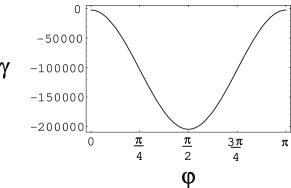
Figure 4: Scalar product $\gamma$ versus the squeezing phase $\varphi$. This refers to a tripartite Gaussian state having CM (28) with parameter choice (29).

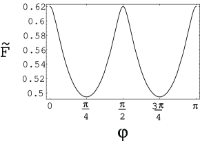
Figure 5: Fidelity $\tilde{F}$ versus the squeezing phase $\varphi$. This refers to a tripartite Gaussian state having CM (28) with parameter choice (29).

V.2.1 Different parameter choice

It is instructive to study a different parameter choice leading to a more involved situation. Setting

$$\{a,b,c,d,e,f\}=\{0.55,0.89,0.94,0.74,0.249,0.12\}$$ (33)

in (28), we have again a genuine CM and a separable reduced state $\rho^{tr}$ for Alice and Bob. However in this case the proposition $p(\varphi)$ is true only for $\varphi\in]\varphi_{1},\varphi_{2}[\ \cup\ ]\varphi_{3},\varphi_{4}[\equiv\mathcal{R}$, where the border points $\varphi_{k}$ are given by $\varphi_{1}=0.339,$ $\varphi_{2}=\pi/2-0.339,$ $\varphi_{3}=\pi/2+0.339,$ and $\varphi_{4}=\pi-0.339$ (see Fig. 6). Maximization over the squeezing phase is given by the maximization of the piecewise continuous function

$$\tilde{F}(\varphi)=\left\{\begin{array}[c]{l}F(\xi_{-}(\varphi),\varphi)\qquad\qquad\qquad\qquad\qquad\qquad\quad\ \mathrm{if}\quad\varphi\in\mathcal{R}\\ F(0,\varphi)=[\det\Gamma^{tr}-k_{x}(\varphi)/k_{y}(\varphi)]^{-1/2}\qquad\mathrm{if}\quad\varphi\in[0,\pi[-\mathcal{R}\end{array}\right.$$ (34)

(see (20) and (18)). In Fig. 7 we see that $F(\xi_{-}(\varphi),\varphi)$ does not have maximum points inside the region $\mathcal{R}$, while $F(0,\varphi)$ has two stationary points $\varphi_{-}=0$ and $\varphi_{+}=\pi/2$ which fall in $[0,\pi[-\mathcal{R}$. They are exactly the ones derived from (21) as we can easily check noting that $\tau_{12}=\tau_{21}=0$ and $\tau_{11}-\tau_{22}<0$ so that $\cos(2\varphi_{\pm})=\mp 1$. It is evident from Fig. 7 that $\varphi_{-}$ is a maximum point while $\varphi_{+}$ is a minimum point for $F(0,\varphi)$. In order to find the global maximum, we have to compare $\tilde{F}(\varphi_{-})=F(0,\varphi_{-})$ with the right and left limits of $\tilde{F}(\varphi)$ at the border points $\varphi_{k}$. Since $\tilde{F}(\varphi_{1})=\tilde{F}(\varphi_{4})=F(\xi_{-}(\varphi_{2}),\varphi_{2})=F(\xi_{-}(\varphi_{3}),\varphi_{3})=0.514,$ $F(0,\varphi_{2})=F(0,\varphi_{3})=0.446$, and $F(0,\varphi_{-})=0.526$, we have that $\bar{\varphi}=\varphi_{-}=0$. In conclusion, in this different parameter choice, the optimal Gaussian measurement at Charlie’s site is the homodyne detection $\left|X(\pi/2)\right\rangle_{c}\left\langle X(\pi/2)\right|$ which implies a fidelity of $52.6\%$ for teleportation of coherent states, and therefore it is again sufficient (together with the classical communication of the result) to create bipartite entanglement between Alice and Bob.

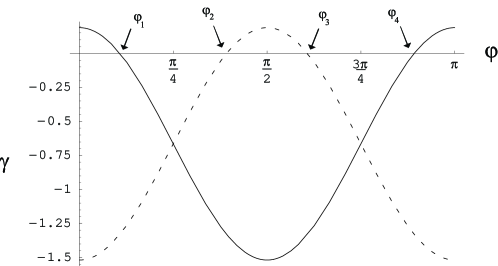
Figure 6: Scalar product $\gamma(\varphi)$ (solid line) and its displaced form $\gamma(\varphi-\pi/2)$ (dashed line) versus the squeezing phase $\varphi$. Denoting with $\varphi_{k}$ ($k=1,2,3,4$) their intersections with the $\varphi$-axis, the proposition $p(\varphi):$ $\gamma(\varphi)<0\wedge$ $\gamma(\varphi-\pi/2)<0$ is true only inside the region $\mathcal{R}\equiv]\varphi_{1},\varphi_{2}[\cup]\varphi_{3},\varphi_{4}[$. This refers to a tripartite Gaussian state having CM (28) with parameter choice (33).

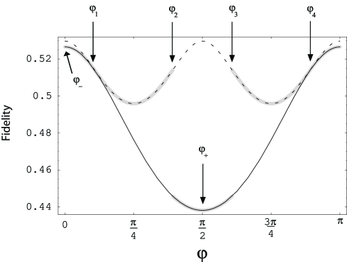
Figure 7: Fidelities $F(\xi_{-}(\varphi),\varphi)$ (dashed line), $F(0,\varphi)$ (solid line) and $\tilde{F}(\varphi)$ (thicker line) versus the squeezing phase $\varphi$. The piecewise continuous function $\tilde{F}(\varphi)$ is discontinuous at points $\varphi_{2}$ and $\varphi_{3}$. This refers to a tripartite Gaussian state having CM (28) with parameter choice (33).

VI Conclusion

We have studied how a two-party teleportation process (between Alice and Bob) within a three-party shared quantum channel can be conditioned by a local measurement and a classical communication of the third party (Charlie). In particular our analysis has been carried out for a shared Gaussian channel, the teleportation of pure Gaussian states, and two general kinds of local measurement at Charlie’s site. We have first shown the case of a dichotomic measurement and we have proved that the non-Gaussian outcome always worsens the fidelity while the Gaussian outcome always improves it, even allowing the conditional generation of entanglement. Then we have shown how the dichotomic measurement can be designed so that the Gaussian outcome optimizes the teleportation fidelity and we have extended such results directly to the case of a local Gaussian measurement at Charlie’s site. From the knowledge of the correlation matrices (the one of the shared tripartite Gaussian state and the one of the state to be teleported), Charlie can always determine and perform an optimal local Gaussian measurement given by a set of squeezed states with squeezing factor $\bar{\xi}(\bar{\varphi})$ and squeezing phase $\bar{\varphi}$, maximizing the fidelity of teleportation of pure Gaussian states between Alice and Bob.

It is an interesting and still open question to establish if this optimal Gaussian measurement is also the best among all possible measurements at Charlie’s site. Proposition 1 shows that in the dichotomic case, the Gaussian outcome yields always a better result than the non-Gaussian one. This fact and also the fact that we are here considering the particular task of teleporting a one mode Gaussian state employing a tripartite Gaussian state suggest that this optimal Gaussian measurement can actually be the best possible measurement Charlie can do to maximize this specific teleportation fidelity. Notice that the recent paper of Ref. Werner has shown that, for $1\rightarrow 2$ cloning of coherent states, even though the joint fidelity is maximized by a Gaussian cloner, the single-copy fidelity is maximized by a non-Gaussian cloner. However, from the point of view of teleportation, the Ref. [21] gives a support to our conjecture that the fidelity of teleportation, for Gaussian input and Gaussian quantum channel, is optimized by a Gaussian measurement. In fact, in Ref. [21], the particular optimal non-Gaussian cloner which realizes $F_{1}=1$ and $F_{2}=0$ (with $F_{k}$ the single-copy fidelity of the $k^{th}$ clone), and therefore gives the optimal quantum teleportation from the coherent input to one clone, actually coincides with a Gaussian cloner (see Fig. 1 in Ref. [21] at the extremal points $(1,0)$ and $(0,1)$).

We finally notice that the procedure sketched in this work can be applied to all CV teleportation networks based on a multipartite Gaussian state and can be used also for the conditional generation of bipartite entanglement.

VII Acknowledgments

Authors thank Jens Eisert for insightful comments.

Appendix A Derivation of the correlation matrix of Eq. (4)

We can derive the CM of Eq. (4) using the symmetrically ordered characteristic function milburn . The measurement operator $\hat{E}_{0}$ is a state of mode $c$ and it can be expressed as

$$\hat{E}_{0}=\pi^{-1}\int\hat{D}_{c}^{\dagger}(\eta_{c})\Phi_{0}(\eta_{c})d^{2}\eta_{c}$$ (35)

where $\hat{D}_{c}(\eta_{c})=\exp(\eta_{c}\hat{c}^{\dagger}-\eta_{c}^{\ast}\hat{c})$ is the displacement operator acting on the Hilbert space of mode $c$, $\Phi_{0}(\eta_{c})$ is the corresponding characteristic function, and $\eta_{c}\equiv\eta_{c}^{R}+i\eta_{c}^{I}$ is a complex variable corresponding to the annihilation operator $\hat{c}$ milburn . Since $\hat{E}_{0}$ is a Gaussian state, we have

$$\Phi_{0}(\vec{\eta}_{c})=\exp(-\vec{\eta}_{c}^{T}V_{0}\vec{\eta}_{c}+i\vec{d}_{0}^{T}\vec{\eta}_{c})$$ (36)

where $V_{0}$ is the CM of the state, $\vec{d}_{0}\in{\mathbb{R}}^{2}$ the displacement, and $\vec{\eta}_{c}^{T}\equiv(\eta_{c}^{I},-\eta_{c}^{R})$ an ${\mathbb{R}}^{2}$ vector connected to $\eta_{c}$. In the same way, the total three-mode Gaussian state

$$\rho=\pi^{-3}\int\int\int\hat{D}_{a}^{\dagger}(\eta_{a})\hat{D}_{b}^{\dagger}(\eta_{b})\hat{D}_{c}^{\dagger}(\eta_{c})\Phi(\eta_{a},\eta_{b},\eta_{c})d^{2}\eta_{a}d^{2}\eta_{b}d^{2}\eta_{c}$$ (37)

is associated to the characteristic function

$$\Phi(\vec{\eta})=\exp(-\vec{\eta}^{T}V\vec{\eta}+i\vec{d}^{T}\vec{\eta})$$ (38)

where $V$ is the CM of Eq. (1), $\vec{d}\in{\mathbb{R}}^{6}$ is the displacement, and $\vec{\eta}^{T}\equiv(\vec{\eta}_{a}^{T},\vec{\eta}_{b}^{T},\vec{\eta}_{c}^{T})$ an ${\mathbb{R}}^{6}$ vector connected to $(\eta_{a},\eta_{b},\eta_{c})$ as shown before.

The conditional reduced state

$$\rho^{(0)}\equiv P_{0}^{-1}\mathrm{Tr}_{c}(\hat{E}_{0}\rho\hat{E}_{0}^{\dagger})$$ (39)

corresponds to a characteristic function $\Phi^{(0)}(\eta_{a},\eta_{b})$ which is (by definition)

$$\Phi^{(0)}(\eta_{a},\eta_{b})\equiv\mathrm{Tr}_{ab}\left[\rho^{(0)}\hat{D}_{a}(\eta_{a})\hat{D}_{b}(\eta_{b})\right]$$ (40)

Putting Eqs. (35) and (37) into Eq. (39), and the subsequent result in Eq. (40), we obtain after some algebra

$$\Phi^{(0)}(\eta_{a},\eta_{b})=\pi^{-2}P_{0}^{-1}\int\int\Phi_{0}(\vartheta)\Phi_{0}(\kappa)\Phi(\eta_{a},\eta_{b},-\vartheta-\kappa)\exp\left(\frac{\vartheta\kappa^{\ast}-\vartheta^{\ast}\kappa}{2}\right)d^{2}\vartheta d^{2}\kappa$$ (41)

Inserting now Eqs. (36) and (38) into Eq. (41), and adopting the ${\mathbb{R}}^{4}$ variable $\vec{\varsigma}^{T}\equiv(\vartheta^{I},-\vartheta^{R},\kappa^{I},-\kappa^{R})$, we obtain

$$\Phi^{(0)}(\vec{\eta}_{a},\vec{\eta}_{b})=\pi^{-2}P_{0}^{-1}\Phi^{tr}(\vec{\eta}_{a},\vec{\eta}_{b})\int\exp(-\vec{\varsigma}^{T}\tilde{M}\vec{\varsigma}+\vec{v}^{T}\vec{\varsigma})d\vec{\varsigma}$$ (42)

where

$$\Phi^{tr}(\vec{\eta}_{a},\vec{\eta}_{b})=\exp\left[-(\vec{\eta}_{a}^{T},\vec{\eta}_{b}^{T})V^{tr}\left(\begin{array}[c]{c}\vec{\eta}_{a}\\ \vec{\eta}_{b}\end{array}\right)+i(\vec{d}^{tr})^{T}\left(\begin{array}[c]{c}\vec{\eta}_{a}\\ \vec{\eta}_{b}\end{array}\right)\right]$$ (43)

is the characteristic function of $\rho^{tr}$,

$$\tilde{M}\equiv\left(\begin{array}[c]{cc}C+V_{0}&C-\frac{i}{2}\Omega\\ C+\frac{i}{2}\Omega&C+V_{0}\end{array}\right)$$ (44)

is a $4\times 4$ matrix expressed in terms of the $2\times 2$ submatrices $V_{0}$, $C$ (Charlie’s submatrix in Eq. (1)) and $\Omega$ (defined in Eq. (7)),

$$\vec{v}\equiv\left(\begin{array}[c]{c}2(E^{T}\vec{\eta}_{a}+D^{T}\vec{\eta}_{b})+i(\vec{d}_{0}-\vec{d}_{c})\\ 2(E^{T}\vec{\eta}_{a}+D^{T}\vec{\eta}_{b})+i(\vec{d}_{0}-\vec{d}_{c})\end{array}\right)$$ (45)

is an ${\mathbb{R}}^{4}$ vector, with $E$ and $D$ the off-diagonal $2\times 2$ submatrices in Eq. (1) and $\vec{d}_{c}$ is the displacement of Charlie’s reduced Gaussian state $\rho_{c}=\mathrm{Tr}_{ab}(\rho)$. Solving the integral in (42), we have

$$\Phi^{(0)}(\vec{\eta}_{a},\vec{\eta}_{b})=P_{0}^{-1}\Phi^{tr}(\vec{\eta}_{a},\vec{\eta}_{b})\frac{\exp\left(\frac{1}{4}\vec{v}^{T}\tilde{M}^{-1}\vec{v}\right)}{\sqrt{g}}$$ (46)

where $g\equiv\det\tilde{M}$ is given in Eq. (6). Inserting now Eq. (43) in Eq. (46), and using $\Phi^{(0)}(\vec{0},\vec{0})=1$ ($\Longleftrightarrow\mathrm{Tr}_{ab}(\rho^{(0)})=1$), we get

$$\Phi^{(0)}(\vec{\eta}_{a},\vec{\eta}_{b})=\exp\left[-(\vec{\eta}_{a}^{T},\vec{\eta}_{b}^{T})V^{(0)}\left(\begin{array}[c]{c}\vec{\eta}_{a}\\ \vec{\eta}_{b}\end{array}\right)+i(\vec{d}^{(0)})^{T}\left(\begin{array}[c]{c}\vec{\eta}_{a}\\ \vec{\eta}_{b}\end{array}\right)\right]$$ (47)

where

$$\vec{d}^{(0)}=\vec{d}^{tr}+\left(\begin{array}[c]{c}EM(\vec{d}_{0}-\vec{d}_{c})\\ DM(\vec{d}_{0}-\vec{d}_{c})\end{array}\right)$$ (48)

is the displacement, with $M$ given in Eq. (5), and the CM $V^{(0)}$ corresponds to the expression of Eq. (4).

Appendix B Proof of Proposition 3

Using vectors $\vec{u}^{T}=(u_{x},u_{y})$ in (12) and $\vec{k}(\varphi)^{T}=(k_{x}(\varphi),k_{y}(\varphi))$ in (13), the fidelity $F(\xi,\varphi)$ can be written as in (18). For an arbitrary $\varphi$, we want to compute the stationary points $\xi_{\pm}(\varphi)$ of $F(\xi,\varphi)$ in the $\xi$ variable. We then introduce the quantity

$$N(\xi,\varphi)\equiv\frac{4\xi^{2}g(\xi,\varphi)^{2}}{F(\xi,\varphi)^{3}}\frac{d}{d\xi}F(\xi,\varphi)$$ (49)

so that they are given by $N(\xi,\varphi)=0$ (for $0<\xi<+\infty$). If the stationary points $\xi_{\pm}(\varphi)$ exist (i.e. they are finite and positive), they have the form

$$\xi_{\pm}(\varphi)=\frac{\omega(\varphi)\pm\sqrt{\Xi(\varphi)}}{\gamma(\varphi-\pi/2)}$$ (50)

with

$$\Xi(\varphi)\equiv\omega(\varphi)^{2}+\gamma(\varphi-\pi/2)\gamma(\varphi)$$ (51)

and $\gamma(\varphi)$ and $\omega(\varphi)$ defined respectively in (14) and (15). From the product

$$\xi_{+}(\varphi)\xi_{-}(\varphi)=-\frac{\gamma(\varphi-\pi/2)\gamma(\varphi)}{\left[\gamma(\varphi-\pi/2)\right]^{2}}$$ (52)

it follows that $\gamma(\varphi-\pi/2)\gamma(\varphi)>0$ implies the existence of only one stationary point ($\xi_{+}(\varphi)$ and $\xi_{-}(\varphi)$ have opposite sign). In particular

$$\gamma(\varphi-\pi/2)<0\wedge\gamma(\varphi)<0\Longrightarrow\xi_{-}(\varphi)>0,$$ (53)

while

$$\gamma(\varphi-\pi/2)>0\wedge\gamma(\varphi)>0\Longrightarrow\xi_{+}(\varphi)>0.$$ (54)

Since

$$N(\xi_{\pm}(\varphi)+\varepsilon,\varphi)=\gamma(\varphi-\pi/2)\varepsilon^{2}\pm 2\sqrt{\Xi(\varphi)}\varepsilon$$ (55)

it is easy to prove that in (53) $\xi_{-}(\varphi)$ is a global maximum ($\equiv\xi_{\max}(\varphi)$) while in (54) $\xi_{+}(\varphi)$ is a global minimum ($\equiv\xi_{\min}(\varphi)$).

Looking at (52), we then analyze the other conditions $\gamma(\varphi-\pi/2)\gamma(\varphi)<0$ and $\gamma(\varphi-\pi/2)\gamma(\varphi)=0$.

• If $\gamma(\varphi-\pi/2)\gamma(\varphi)<0$ then $\xi_{+}(\varphi)$ and $\xi_{-}(\varphi)$ are different from zero and have the same sign. Suppose that $\xi_{\pm}(\varphi)>0$ and consider the case $\gamma(\varphi-\pi/2)<0\wedge\gamma(\varphi)>0$ (the proof is analogous in the other case $\gamma(\varphi-\pi/2)>0\wedge\gamma(\varphi)<0$). From (50) it follows that $\omega(\varphi)<0$. On the other hand, from $\gamma(\varphi)=u_{x}k_{x}(\varphi)+u_{y}k_{y}(\varphi)>0$ and $\gamma(\varphi-\pi/2)=u_{x}k_{x}(\varphi-\pi/2)+u_{y}k_{y}(\varphi-\pi/2)<0$, it follows that $k_{x}(\varphi)k_{y}(\varphi-\pi/2)-k_{y}(\varphi)k_{x}(\varphi-\pi/2)=2\omega(\varphi)>0$ which is impossible. For this reason $\gamma(\varphi-\pi/2)\gamma(\varphi)<0$ implies the non existence of the stationary points $\xi_{\pm}(\varphi)$. Now, since the extended function $F(\xi,\varphi)$ surely has a maximum and a minimum, the global extremal points $\xi_{\min}(\varphi)$ and $\xi_{\max}(\varphi)$ must be the two border points $0$ or $+\infty$.

The last condition to be analyzed, i.e. $\gamma(\varphi-\pi/2)\gamma(\varphi)=0$, must be distinguished in more cases.

• First suppose that $\gamma(\varphi-\pi/2)=\gamma(\varphi)=0$. Using this condition in (18), it leads to $F(\xi,\varphi)=\left[\det\Gamma^{tr}-k_{x}(\varphi)/k_{y}(\varphi)\right]^{-1/2}$, making the fidelity $\xi-$independent, so that we can freely choose $\xi_{\min}(\varphi)$ and $\xi_{\max}(\varphi)$ at the border.

• Next suppose that $\gamma(\varphi-\pi/2)\neq 0\wedge\gamma(\varphi)=0$. In such case $\gamma(\varphi)=0\Longrightarrow$ $\omega(\varphi)=-[k_{y}(\varphi)/2u_{x}]\gamma(\varphi-\pi/2)$ and since $k_{y}(\varphi)>0$, $u_{x}>0$ we have that $\omega(\varphi)$ and $\gamma(\varphi-\pi/2)$ have opposite signs. On the other hand $\gamma(\varphi)=0\Longrightarrow\xi_{\pm}(\varphi)=\left[\omega(\varphi)\pm\left|\omega(\varphi)\right|\right]/\gamma(\varphi-\pi/2)$. Consider now $\gamma(\varphi-\pi/2)>0$ (the proof is analogous in the other case $\gamma(\varphi-\pi/2)<0$), therefore $\omega(\varphi)<0$ and we have $\xi_{-}(\varphi)=2\omega(\varphi)/\gamma(\varphi-\pi/2)=-k_{y}(\varphi)/u_{x}<0$ while $\xi_{+}(\varphi)=0$, concluding that stationary points do not exist (global extremal points at the border).

• Finally the case $\gamma(\varphi-\pi/2)=0\wedge\gamma(\varphi)\neq 0$ can be taken back to the previous ones using periodicity arguments. Setting $\tilde{\varphi}\equiv\varphi-\pi/2$ in the last logic proposition, we achieve $\gamma(\tilde{\varphi})=0\wedge\gamma(\tilde{\varphi}+\pi/2)\neq 0$, from which we can derive both $\gamma(\tilde{\varphi}-\pi/2)=\gamma(\tilde{\varphi})=0$ and $\gamma(\tilde{\varphi}-\pi/2)\neq 0\wedge\gamma(\tilde{\varphi})=0$. In either cases we have $\left(\xi_{\min}(\tilde{\varphi})=0\wedge\xi_{\max}(\tilde{\varphi})=+\infty\right)\vee\left(\xi_{\min}(\tilde{\varphi})=+\infty\wedge\xi_{\max}(\tilde{\varphi})=0\right)$. From (19) we have $F(\xi,\tilde{\varphi})=F(\xi^{-1},\tilde{\varphi}+\pi/2)=F(\xi^{-1},\varphi)$ and therefore $\left(\xi_{\min}(\varphi)=+\infty\wedge\xi_{\max}(\varphi)=0\right)\vee\left(\xi_{\min}(\varphi)=0\wedge\xi_{\max}(\varphi)=+\infty\right)$.

In conclusion we can summarize all the cases as follows:

$$\gamma(\varphi-\pi/2)\gamma(\varphi)\leq 0\Longleftrightarrow\left(\xi_{\min}(\varphi)=+\infty\wedge\xi_{\max}(\varphi)=0\right)\vee\left(\xi_{\min}(\varphi)=0\wedge\xi_{\max}(\varphi)=+\infty\right)$$ (56)

$$\gamma(\varphi-\pi/2)>0\wedge\gamma(\varphi)>0\Longleftrightarrow\xi_{\min}(\varphi)=\xi_{+}(\varphi)\wedge(\xi_{\max}(\varphi)=0\vee\xi_{\max}(\varphi)=+\infty)$$ (57)

$$\gamma(\varphi-\pi/2)<0\wedge\gamma(\varphi)<0\Longleftrightarrow\xi_{\max}(\varphi)=\xi_{-}(\varphi)\wedge(\xi_{\min}(\varphi)=0\vee\xi_{\min}(\varphi)=+\infty)$$ (58)

from which we derive propositions (16) and (17) when we consider only the global maximum point $\xi_{\max}(\varphi)\equiv\bar{\xi}(\varphi)$.

References

- (1) S. L. Braunstein and H. J. Kimble, Phys. Rev. Lett. 80, 869 (1998); A. Furusawa et al., Science 282, 706 (1998); W. P. Bowen, N. Treps, B. C. Buchler, R. Schnabel, T. C. Ralph, H.-A. Bachor, T. Symul, and P. K. Lam Phys. Rev. A 67, 032302 (2003); T. C. Zhang, K. W. Goh, C. W. Chou, P. Lodahl, and H. J. Kimble Phys. Rev. A 67, 033802 (2003).
- (2) F. Grosshans et al., Nature (London) 421, 238 (2003).
- (3) P. van Loock and S. L. Braunstein, Phys. Rev. Lett. 84, 3482 (2000); ibid. 87, 247901 (2001).
- (4) A. Ferraro, M. G. A. Paris, M. Bondani, A. Allevi, E. Puddu, A. Andreoni , J. Opt. Soc. Am. B 21, 1241 (2004).
- (5) S. Mancini et al., Phys. Rev. Lett. 90, 137901 (2003).
- (6) S. Pirandola et al., Phys. Rev. A 68, 062317 (2003).
- (7) S. Pirandola et al., J. Mod. Opt. 51, 901 (2004).
- (8) S. Pirandola et al., J. Opt. B: Quantum Semiclassical Opt 5, S523 (2003).
- (9) J. Jing, J. Zhang, Y. Yan, F. Zhao, C. Xie, and K. Peng, Phys. Rev. Lett. 90, 167903 (2003); T. Aoki, N. Takei, H. Yonezawa, K. Wakui, T. Hiraoka, A. Furusawa, and P. van Loock, Phys. Rev. Lett. 91, 080404 (2003).
- (10) A. M. Lance, T. Symul, W. P. Bowen, B. C. Sanders, and P. K. Lam, Phys. Rev. Lett. 92, 177903 (2004).
- (11) H. Yonezawa, T. Aoki, and A. Furusawa, Nature (London) 431, 430 (2004).
- (12) J. Fiurášek, Phys. Rev. A 66, 012304 (2002).
- (13) J. Eisert, S. Scheel, and M. B. Plenio, Phys. Rev. Lett. 89, 137903 (2002); G. Giedke and J.I. Cirac, Phys. Rev. A 66, 032316 (2002).
- (14) Note that both fidelities and are conditional quantities; the first one corresponds to the selection of a particular outcome of the measurement, while the second one does not depend on the outcome but it is determined by the kind of measurement chosen by Charlie.
- (15) Conditioning reduces entropy i.e , where is the Von Neumann entropy. See for instance: M. A. Nielsen and I. L. Chuang, Quantum Computation and Quantum Information, Cambridge University Press, Cambridge, 2000).
- (16) L.-M. Duan et al., Phys. Rev. Lett. 84, 2722 (2000).
- (17) D. F. Walls and G. J. Milburn, Quantum Optics, (Springer, Berlin, 1994).
- (18) G. Giedke, B. Kraus, M. Lewenstein, and J. I. Cirac, Phys. Rev. A 64, 052303 (2001).
- (19) S. Pirandola, Int. J. Quant. Inf. 3, 239-243 (2005).
- (20) R. Simon, Phys. Rev. Lett. 84, 2726 (2000).
- (21) N.J. Cerf, O. Krüger, P. Navez, R.F. Werner, and M.M. Wolf, e-print quant-ph/0410058v2.