Abstract

We present a quantum theory of nondegenerate phase-sensitive parametric amplification in a $\chi^{(3)}$ nonlinear medium. The non-zero response time of the Kerr $(\chi^{(3)})$ nonlinearity determines the quantum-limited noise figure of $\chi^{(3)}$ parametric amplification, as well as the limit on quadrature squeezing. This non-zero response time of the nonlinearity requires coupling of the parametric process to a molecular-vibration phonon bath, causing the addition of excess noise through spontaneous Raman scattering. We present analytical expressions for the quantum-limited noise figure of frequency non-degenerate and frequency degenerate $\chi^{(3)}$ parametric amplifiers operated as phase-sensitive amplifiers. We also present results for frequency non-degenerate quadrature squeezing. We show that our non-degenerate squeezing theory agrees with the degenerate squeezing theory of Boivin and Shapiro as degeneracy is approached. We have also included the effect of linear loss on the phase-sensitive process.

OCIS codes: 060.2320, 270.5290.

1 Introduction

Fiber-optical parametric amplifiers (FOPAs) are currently the subject of much research for use in wavelength conversion[1] and efficient broadband amplification[2]. They are also candidates for performing all-optical network functions[3, 4, 5]. Advances in pumping techniques have permitted improvements of the noise figure (NF) of FOPAs operated phase-insensitively [1, 6] and the manufacture of high-nonlinearity and microstructure fibers has improved the gain slope[7, 8] of FOPAs.

In order to explain our experimental noise figure result for a FOPA operated as a phase-insensitive amplifier (PIA) [9], we have recently published a quantum theory of $\chi^{(3)}$ parametric amplifiers that takes into account the non-instantaneous nonlinear response of the medium and the requisite addition of noise caused by this non-instantaneous nonlinear response [10, 11]. The FOPA operates as a PIA when an idler beam is generated wholly in the fiber or when the phase difference (twice the phase of the pump less the phases of the Stokes and anti-Stokes beams) is approximately $0$ or $\pi$ and the Stokes and anti-Stokes beams are approximately equal in amplitude. Our work with FOPAs operated as PIAs also provides analytical expressions for the noise figure of $\chi^{(3)}$ phase-insensitive parametric amplifiers [10] and wavelength converters [11]. This theory shows excellent agreement with experiment [9]. In addition, we have recently experimentally investigated the noise figure spectrum for PIA and wavelength converter operation of a FOPA, and shown good agreement to an extended theory that includes distributed loss[12]. This inclusion of distributed loss was necessary to model the experiment[12], but also provides the necessary quantum theory for predicting the performance of a distributed amplifier.

Phase-sensitive amplifiers (PSA) [13, 14] are also of interest because unlike PIAs, they can ideally provide amplification without degrading the signal-to-noise ratio (SNR) at the input[15]. Operation of a FOPA as a PSA occurs when the phase difference at the input is approximately $\pi/2$ and the signal and idler are approximately equal in amplitude. Experiments with fully frequency degenerate fiber phase-sensitive amplifiers have demonstrated a noise figure of $2.0$ dB at a gain of $16$ dB [16], a value lower than the standard phase-insensitive high-gain $3$-dB quantum limit. A noise figure below the standard PIA limit has also been reached in a low-gain phase-sensitive amplifier [17]. However, these fully frequency degenerate PSA experiments were impaired by guided-acoustic-wave Brillouin scattering (GAWBS)[18] requiring pulsed operation [19] or sophisticated techniques for partially suppressing GAWBS [17]. In order to avoid the GAWBS noise one may obtain phase-sensitive amplification with an improved experimental noise figure by use of a frequency nondegenerate PSA. In addition, the nondegenerate PSA, unlike its degenerate counterpart, can be used with multiple channels of data. A nondegenerate PSA is realized by placing the signal in two distinct frequency bands symmetrically around the pump frequency with a separation of several GHz, so that GAWBS noise scattered from the pump is not in the frequency bands of the signal. Such frequency nondegenerate regime has been demonstrated experimentally, showing good agreement with theory for the average values of the signal and idler[20]. We have also experimentally demonstrated an improved bit-error rate by use of a PSA as opposed to a PIA of comparable gain[21]. However, quantum-limited noise figure measurements have yet to be performed. So an analysis of this case is practically useful. Accordingly, we here describe in suitable detail a quantum theory of FOPAs that takes into account the non-zero response time of the $\chi^{(3)}$ nonlinearity along with the effect of distributed linear loss. We present analytical expressions for the quantum-limited noise figure of CW $\chi^{(3)}$ PSAs in the frequency nondegenerate case. We also report the limiting value of the NF when degeneracy is approached. In addition, we note that this theory is valid for FOPAs used as distributed phase-sensitive amplifiers [22].

A frequency nondegenerate parametric amplifier can also operate as a phase-sensitive deamplifier (PSD) of two-frequency input signals. This occurs when the phase-difference at the input is approximately $-\pi/2$ and the Stokes and anti-Stokes inputs are approximately equal in amplitude. When a PSD is operated with no input signal, such a parametric amplifier is said to produce “quadrature-squeezed vacuum” (parametric fluorescence of the PSD) whose two-frequency homodyne detection exhibits photocurrent variance less than that of the vacuum for suitable choice of homodyne phases [23]. Quadrature squeezing has been proposed for applications in quantum communications [24, 25, 26], improved measurement sensitivity [27, 28], and quantum lithography[29]. In the case of FOPAs, previous work by Shapiro and Boivin [30] used the dispersionless theory of self-phase modulation developed by Boivin and Kärtner  [31, 32] that included the non-instantaneous response of the $\chi^{(3)}$ nonlinearity to obtain a limit on quadrature squeezing in the fully four-degenerate-wave case. In this paper, we present results for frequency nondegenerate CW quadrature squeezing for a noninstantaneous nonlinearity in the presence of dispersion. We show that optimal squeezing occurs for slightly different input conditions than those for optimal classical deamplification. In addition, we show that, unlike the dispersionless case, the degree of squeezing reaches a constant value in the long-interaction-length limit when the linear phase-mismatch is nonzero and a non-instantaneous nonlinear response is present. Our nondegenerate squeezing theory agrees with the previous degenerate squeezing results of Boivin and Shapiro [30] when degeneracy is approached.

This paper is organized as follows: In Section 2 we discuss the solution of the equations describing evolution of the mean values of the pump, Stokes, and anti-Stokes fields. In Section 3, we present a quantum mechanically consistent theory of the FOPAs. For calculation of the noise figure in phase-sensitive operation, we need to obtain only the mean and variance of the total photocurrent at the Stokes and anti-Stokes wavelengths. Thus we chose to calculate only the output Heisenberg annihilation operators for the Stokes and anti-Stokes frequency-pair of interest. We thus obtain the desired results in a simpler way than had we used the Wigner or positive-P formalism developed by Drummond and Corney[33] for propagation of the quantum states of pulses in the fiber. In Sections 4 and 5, we apply this theory to obtain the noise figure of phase-sensitive amplification and to obtain the degree of nondegenerate quadrature squeezing, respectively. We reemphasize the main results and conclude in Section 6.

2 Classical phase-sensitive amplification and deamplification

We have discussed the $\chi^{(3)}$ nonlinear response at length [11]; only a very brief summary is presented here.

The nonlinear refractive index of the Kerr interaction can be written as

$$n_{2}=\frac{3\chi^{(3)}}{4\epsilon_{0}n_{0}^{2}c},$$ (1)

where $n_{0}$ is the linear refractive index of the nonlinear material, $\epsilon_{0}$ is the permittivity of free space, and $c$ is the speed of light in free space. For clarity, we state that

$$\chi^{(3)}\equiv\chi^{(3)}_{1111}\left[\frac{{\rm m}^{2}}{{\rm V}^{2}}\right].$$ (2)

The $\chi^{(3)}(t)$ nonlinear response is composed of a time-domain delta-function-like electronic response ($\ll 1\,{\rm fs}$) that is constant in the frequency domain over the bandwidths of interest and a time-delayed Raman response ($\approx 50\,{\rm fs}$) that varies over frequencies of interest and is caused by back action of nonlinear nuclear vibrations on electronic vibrations. Recent experimental and theoretical results demonstrate that the nonlinear response function $\chi^{(3)}(t)$ can be treated as if it were real in the time domain, [34, 35] yielding a real part that is symmetric in the frequency domain with respect to pump detuning and an imaginary part in the frequency domain that is anti-symmetric.

Although a nonlinear response is also present in the polarization orthogonal to that of the pump, this cross-polarized nonlinear interaction is ignored because we assume that the pump, Stokes, and anti-Stokes fields of interest stay copolarized as their polarization states evolve during propagation through the FOPA. Parametric fluorescence and Raman spontaneous emission are present in small amounts in the polarization perpendicular to the pump, but do not affect the NF of the amplifier.

We can write $N_{2}(\Omega)$ in the frequency domain as a sum of electronic and molecular contributions:

$$N_{2}(\Omega)=n_{2\rm{e}}+n_{2\rm{r}}F(\Omega).$$ (3)

We also define a nonlinear coefficient $\gamma_{\Omega}$ to be

$${\gamma_{\Omega}=\frac{2\pi N_{2}(\Omega)}{\lambda A_{\rm{eff}}}{\left[\frac{1}{W\cdot m}\right]}},$$ (4)

where $\lambda$ is the pump wavelength and $A_{\rm{eff}}$ is the fiber effective area. Thus our $\gamma_{0}$ is equivalent to the nonlinear coupling coefficient $\gamma$ used in Agrawal [36]. It is the scaling of $A_{\rm eff}$ with wavelength that mainly causes $\gamma_{\Omega}$ to be no longer anti-symmetric with $\gamma_{-\Omega}$ at detunings greater than several THz. In what follows, our analytical treatment of the mean fields allows for the more general case of asymmetry in the Raman-gain spectrum. However, other results including graphs assume an anti-symmetric Raman spectrum as this has a minor effect on the quantum noise at large detunings.

We next present solutions to the mean field equations governing a parametric amplifier. The optical fields are assumed to propagate in a dispersive, polarization-preserving, single-transverse-mode fiber under the slowly-varying-envelope approximation. As the involved waves are quite similar in frequency, to good approximation all fields can be treated as if their transverse mode profiles are idententical. Even though the fibers used to construct FOPAs typically support two polarization modes and the polarization state of the waves is usually elliptical at a given point $z$ in the FOPA, for typical fibers it is still appropriate to describe the system with a scalar theory if the detuning is relatively small[12]. This is because the input waves are copolarized at the beginning of the amplifier and the fields of interest remain essentially copolarized during propagation down the fiber.

Consider the field

$${A}(t)={A}_{p}+{A}_{s}\exp(i\Omega t)+{A}_{a}\exp(-i\Omega t)$$ (5)

for the total field propagating through a FOPA having a frequency and polarization degenerate pump. Here $|A|^{2}$ has units of Watts.The lower frequency field we refer to as the Stokes field, ${A}_{s}$; the higher frequency field referred to as the anti-Stokes field, ${A}_{a}$. The classical equation of motion for the total field[37] with the addition of arbitrary frequency dependent loss is:

$$\frac{\partial{A}(t)}{\partial z}=i\left[\int{\textrm{ d}}\tau\,\gamma(t-\tau){A}^{*}(\tau){A}(\tau)\right]{A}(t)-\int\frac{\alpha(\Omega)}{2}\widetilde{A}(\Omega)\exp(-i\Omega t)\,{\rm d}\Omega,$$ (6)

where $\alpha(\Omega)$ is the power attenuation coefficient at detuning $\Omega$ from the pump and $\widetilde{A}(\Omega)$ is the Fourier transform of the field. Because the involved waves (Stokes, anti-Stokes, and pump) are CW, the usual group-velocity dispersion term does not explicitly appear in Eq. (6). However, dispersion is included; its effect is simply to modify the wavevector of each CW component. Taking the Fourier transform of Eq. (6) and separating into frequency-shifted components that are capable of phase-matching, we obtain the following differential equations for the mean fields [37]:

$$\frac{{\rm{d}}{A}_{p}}{{\rm{d}}z} = i\,\gamma_{0}\,|{A}_{p}|^{2}{A}_{p}-\frac{\alpha_{p}}{2}{A}_{p},$$ (7)

$$\frac{{\rm{d}}{A}_{a}}{{\rm{d}}z} = i\,(\gamma_{0}+\gamma_{\Omega})\,|{A}_{p}|^{2}{A}_{a}+i\gamma_{\Omega}{A}_{p}^{2}{A}_{s}^{*}\exp{(-i\Delta kz)}-\frac{\alpha_{a}}{2}{A}_{a},$$ (8)

$$\frac{{\rm{d}}{A}_{s}}{{\rm{d}}z} = i\,(\gamma_{0}+\gamma_{-\Omega})\,|{A}_{p}|^{2}{A}_{s}+i\gamma_{-\Omega}{A}_{p}^{2}{A}_{a}^{*}\exp{(-i\Delta kz)}-\frac{\alpha_{s}}{2}{A}_{s}.$$ (9)

Here $\Delta k=k_{a}+k_{s}-2k_{p}$ is the phase mismatch. Expanding the wavevectors in a Taylor series around the pump frequency to second order, one obtains $\Delta k=\beta_{2}\Omega^{2}$ to second order, where $\beta_{2}$ is the group-velocity dispersion coefficient. The attenuation coefficients are $\alpha_{j}$ for $j=p,a,s$ at the pump, anti-Stokes, and Stokes wavelenths, respectively. The nonlinear coupling coefficients $\gamma_{0}$, $\gamma_{\Omega}$, and $\gamma_{-\Omega}$ are as defined in the previous section. Eqs. (7–9) are valid when the pump remains essentially undepleted by the Stokes and anti-Stokes waves and is much stronger than the Stokes and anti-Stokes waves. The solution to Eqs. (7) and (9) can be expressed as

$${A}_{a}(z,L) = \mu_{a}(z,L){A}_{a}(z)+\nu_{a}(z,L){A}_{s}^{*}(z),$$ (10)

$${A}_{s}(z,L) = \mu_{s}(z,L){A}_{s}(z)+\nu_{s}(z,L){A}_{a}^{*}(z),$$ (11)

where we have explicitly written the solution as a function of both a starting point $z$ for the parametric process and an end point $L$ for the fiber. We do this because we will be interested not only in the input-output relationships of the electromagnetic fields, i.e. $A_{a}(0,L)$, but also evolution of noise generated at a point $z$ that propagates to the end of the fiber, $L$. In the following subsections, we provide expressions for $\mu_{j}(z,L)$ and $\nu_{j}(z,L)$ for the three main cases of interest.

2.A Distributed loss solution

In the most general case, when there are no restrictions on $\Delta k$ and distributed linear loss is present, Eqs. (7–9) can be shown to have a series solution. We here briefly outline the derivation of this solution. Solving for the mean field of the pump, Eq. (7), we obtain

$${A}_{p}(z)=\exp[i\gamma_{0}I_{p}(0)z_{\rm eff}-\frac{\alpha_{p}z}{2}]{{A}_{p}(0)},$$ (12)

where the effective length $z_{\rm eff}$ is defined to be $z_{\rm eff}=[1-\exp(-\alpha_{p}z)]/\alpha_{p}$. Further defining the initial pump power in Watts to be $I_{p}(0)=|{A}_{p}(0)|^{2}$, and setting the reference phase to be that of the pump at the input of the fiber, we substitute the resulting expressions into Eqs. (8) and (9). Writing

$$\bar{A}_{a} = {B}_{a}\exp[i(\gamma_{0}+\gamma_{\Omega})I_{p}(0)z_{\rm eff}-\alpha_{a}z/2],$$ (13)

$$\bar{A}_{s} = {B}_{s}\exp[i(\gamma_{0}+\gamma_{-\Omega})I_{p}(0)z_{\rm eff}-\alpha_{s}z/2],$$ (14)

and making a change of variable from $z$ to $z_{\rm eff}$, one obtains

$$\frac{{\rm{d}}{B}_{a}}{{\rm{d}}z_{\rm eff}} = i\gamma_{\Omega}I_{p}(0)\exp[-f(z_{\rm eff})]{B}_{s}^{*},$$ (15)

$$\frac{{\rm{d}}{B}_{s}^{*}}{{\rm{d}}z_{\rm eff}} = -i\gamma_{-\Omega}^{*}I_{p}(0)\exp[f(z_{\rm eff})]{B}_{a},$$ (16)

where

$$f(z_{\rm eff})=i[\gamma_{\Omega}+\gamma_{-\Omega}^{*}]I_{p}(0)z_{\rm eff}-\frac{(\alpha_{s}-\alpha_{a}+2i\Delta k)\ln(1-\alpha_{p}z_{\rm eff})}{2\alpha_{p}}.$$ (17)

After some algebra and making use of the substitutions

$$\bar{F}_{a} = {B_{a}}\exp[f(z_{\rm eff})],$$ (18)

$$\bar{F}_{s}^{*} = {B}_{s}^{*}\exp[-f(z_{\rm eff})],$$ (19)

we can obtain the nonlinear coupled equations

$$\frac{{\rm{d}}{F}_{a}}{{\rm{d}}z_{\rm eff}}-[\Gamma+\frac{\Lambda}{1-\alpha_{p}z_{\rm eff}}]{F}_{a} = \xi_{1}{F}_{s}^{*},$$ (20)

$$\frac{{\rm{d}}{F}_{s}^{*}}{{\rm{d}}z_{\rm eff}}+[\Gamma+\frac{\Lambda}{1-\alpha_{p}z_{\rm eff}}]\bar{F}_{s}^{*} = \xi_{2}{F}_{a},$$ (21)

where the following constants are used for calculating evolution from point $z$ to $L$: $\Gamma=i[\gamma_{\Omega}+\gamma_{-\Omega}^{*}]I_{p}(z)/2$, $\Lambda=[\alpha_{s}/2-\alpha_{a}/2+i\Delta k]/2$, $\xi_{1}=i\gamma_{\Omega}I_{p}(z)$, and $\xi_{2}=-i\gamma_{-\Omega}^{*}I_{p}(z)$. Using the expansion

$$\frac{1}{1-\alpha_{p}z_{\rm eff}}=\sum_{n=0}^{\infty}\alpha_{p}^{n}z_{\rm eff}^{n},$$ (22)

on the nonlinear term in Eqs. (20) and (21), we find a series solution for ${F}_{j}$ and then obtain ${A}_{j}$.

The series solution converges in relatively few terms when $\alpha_{p}z_{\rm eff}$ is small, which is the case for practical amplifiers. The following solutions are then obtained:

$$\mu_{a}(z,L) = \exp[p(z,L)]\sum_{n=0}^{\infty}a_{n}L_{\rm eff}^{n}\,\,\,\,\,({a_{0}=1,s^{*}_{0}=0}),$$ (23)

$$\mu_{s}(z,L) = \exp[p(z,L)]\sum_{n=0}^{\infty}s_{n}L_{\rm eff}^{n}\ \,\,\,\,\,{(a_{0}=0,s^{*}_{0}=1)},$$ (24)

$$\nu_{a}(z,L) = \exp[p(z,L)]\sum_{n=0}^{\infty}a_{n}L_{\rm eff}^{n}\,\,\,\,\,({a_{0}=0,s^{*}_{0}=1}),$$ (25)

$$\nu_{s}(z,L) = \exp[p(z,L)]\sum_{n=0}^{\infty}s_{n}L_{\rm eff}^{n}\,\,\,\,\,({a_{0}=1,s^{*}_{0}=0}),$$ (26)

where

$$p(z,L) = i[\gamma_{0}+(\gamma_{\Omega}-\gamma_{-\Omega}^{*})/2]I_{p}(z)L_{\rm eff}$$ (28)

$$-i\Delta k(L-z)/2-\alpha_{a}(L-z)/4-\alpha_{s}(L-z)/4$$

and $L_{\rm eff}=\{1-\exp[-\alpha_{p}(L-z)]\}/\alpha_{p}$. The coefficients $a_{n}$ and $s^{*}_{n}$ are then calculated through the following recursion relations:

$$a_{n} = \frac{\Gamma a_{n-1}+\xi_{1}s^{*}_{n-1}+\Lambda\sum_{j=0}^{n-1}\alpha_{p}^{j}a_{n-1-j}}{n},$$ (29)

$$s^{*}_{n} = \frac{-\Gamma s^{*}_{n-1}+\xi_{2}a_{n-1}-\Lambda\sum_{j=0}^{n-1}\alpha_{p}^{j}s^{*}_{n-1-j}}{n}.$$ (30)

2.B Lossless, $\Delta k\neq 0$ solution

The solution for lossless fiber and $\Delta k\neq 0$ is well known, as are the $\mu$ and $\nu$ functions which can be expressed as[37]

$$\mu_{a}(z,L) = \exp\left(-\frac{i\left(\Delta k-[2\gamma_{0}+\gamma_{\Omega}-\gamma_{-\Omega}^{*}]I_{p}\right)(L-z)}{2}\right)$$ (31)

$$\times\left(\frac{i\kappa}{2g}\sinh[g(L-z)]+\cosh[g(L-z)]\right),$$

$$\mu_{s}(z,L) = \exp\left(-\frac{i\left(\Delta k-[2\gamma_{0}+\gamma_{-\Omega}-\gamma_{\Omega}^{*}]I_{p}\right)(L-z)}{2}\right)$$ (32)

$$\left(\frac{i\kappa^{*}}{2g^{*}}\sinh[g^{*}(L-z)]+\cosh[g^{*}(L-z)]\right),$$

$$\nu_{a}(z,L) = \exp\left(-\frac{i\left(\Delta k-[2\gamma_{0}+\gamma_{\Omega}-\gamma_{-\Omega}^{*}]I_{p}\right)(L-z)}{2}\right)\frac{i\gamma_{\Omega}{A_{p}(z)^{2}}{}}{g}\sinh[g(L-z)],$$

$$\nu_{s}(z,L) = \exp\left(-\frac{i\left(\Delta k-[2\gamma_{0}+\gamma_{-\Omega}-\gamma_{\Omega}^{*}]I_{p}\right)(L-z)}{2}\right)\frac{i\gamma_{-\Omega}{A_{p}(z)^{2}}{}}{g^{*}}\sinh[g^{*}(L-z)].$$

Here $I_{p}(z)=I_{p}=|{A}_{p}(0)|^{2}$ is the pump power in Watts, $\kappa=\Delta k+(\gamma_{\Omega}+\gamma_{-\Omega}^{*})I_{p}$, and $g=\sqrt{-(\kappa/2)^{2}+\gamma_{\Omega}\gamma_{-\Omega}^{*}I_{p}^{2}}$ is the complex gain coefficient.

2.C Lossless, $\Delta k=0$ solution

We also state the results for the lossless, $\Delta k=0$ case, which is useful in our analysis near degeneracy. We have $\Delta k=0$ when the FOPA is pumped at the zero dispersion wavelength or if the system is treated as if dispersionless. When the three frequencies are very nearly degenerate, we can also make the approximation that $\Delta k=0$. Then the $\mu$ and $\nu$ functions become

$$\mu_{a}(z,L) = \exp\left[i\left(\frac{2\gamma_{0}+\gamma_{\Omega}-\gamma_{-\Omega}^{*}}{2}\right)I_{p}(L-z)\right][1+i\gamma_{\Omega}{(L-z)}I_{p}],$$ (35)

$$\mu_{s}(z,L) = \exp\left[i\left(\frac{2\gamma_{0}+\gamma_{-\Omega}-\gamma_{\Omega}^{*}}{2}\right)I_{p}(L-z)\right][1+i\gamma_{-\Omega}{(L-z)}I_{p}],$$ (36)

$$\nu_{a}(z,L) = \exp\left[i\left(\frac{2\gamma_{0}+\gamma_{\Omega}-\gamma_{-\Omega}^{*}}{2}\right)I_{p}(L-z)\right]i\gamma_{\Omega}{(L-z)A_{p}(z)^{2}},$$ (37)

$$\nu_{s}(z,L) = \exp\left[i\left(\frac{2\gamma_{0}+\gamma_{-\Omega}-\gamma_{\Omega}^{*}}{2}\right)I_{p}(L-z)\right]i\gamma_{-\Omega}{(L-z)A_{p}(z)^{2}}.$$ (38)

Under the normal assumption of an anti-symmetric Raman gain profile ($\gamma_{\Omega}=\gamma_{-\Omega}^{*}$), we see the power gain for an input only on the anti-Stokes side, $G_{anti-Stokes}=|\mu_{a}(0,L)|^{2}=1-2{\rm Im}\{\gamma_{\Omega}\}I_{p}L+|\gamma_{\Omega}|^{2}I_{p}^{2}L^{2}$, has a four wave mixing gain that is quadratic as a function of fiber length and that the Raman loss at the anti-Stokes wavelength is linear in pump power and length ($-2{\rm Im}\{\gamma_{\Omega}\}I_{p}L$). Similarly, the Raman gain at the Stokes wavelength is linear in power and length ($2{\rm Im}\{\gamma_{-\Omega}\}I_{p}L$).

2.D Optimal classical phase-sensitive amplification and deamplification

We next find the optimal phase-sensitive amplification and phase-sensitive deamplification of a mean field consisting of a superposition of Stokes and anti-Stokes fields. We define optimal phase-sensitive amplification (deamplification) as the greatest (least) output signal power possible for a fixed amount of input signal power. Assuming coherent signal inputs $\zeta_{j}$ having powers $|\zeta_{j}|^{2}$ and phases $\exp(i\theta_{j})$ for $j=a,s$, the phase-sensitive gain of the PSA is

$$G = \frac{|{A}_{a}(L)|^{2}+|{A}_{s}(L)|^{2}}{|{A}_{a}(0)|^{2}+|{A}_{s}(0)|^{2}}$$

$$= \frac{|\mu_{a}\zeta_{a}+\nu_{a}\zeta_{s}^{*}|^{2}+|\mu_{s}\zeta_{s}+\nu_{s}\zeta_{a}^{*}|^{2}}{|\zeta_{a}|^{2}+|\zeta_{s}|^{2}}$$

$$= \frac{(|\mu_{a}|^{2}+|\nu_{s}|^{2})|\zeta_{a}|^{2}+(|\nu_{a}|^{2}+|\mu_{s}|^{2})|\zeta_{s}|^{2}+\left\{[(\mu_{s}\nu_{s}^{*}+\mu_{a}\nu_{a}^{*})|\zeta_{a}||\zeta_{s}|\,\,e^{i(\theta_{a}+\theta_{s})}]+{\rm c.c.}\right\}}{|\zeta_{a}|^{2}+|\zeta_{s}|^{2}}.$$

By properly choosing the relative power of the Stokes and anti-Stokes inputs and their sum phase $\theta=\theta_{a}+\theta_{s}$ relative to the input pump phase, one achieves maximimum (minimimum) phase-sensitive amplification (deamplification). The optimum sum phases $\theta_{\rm psa,\,\,opt}$ and $\theta_{\rm psd,\,\,opt}$ are

$$\theta_{\rm psa,\,\,opt}=-\arg[\mu_{s}\nu_{s}^{*}+\mu_{a}\nu_{a}^{*}],$$ (40)

$$\theta_{\rm psd,\,\,opt}=\pi-\arg[\mu_{s}\nu_{s}^{*}+\mu_{a}\nu_{a}^{*}],$$ (41)

for amplification and deamplification, respectively. By setting the sum input power $|\zeta_{a}|^{2}+|\zeta_{s}|^{2}=\mathcal{C}$ to be some constant $\mathcal{C}$, the extrema of Eq. (LABEL:psa_mean_out) can be found to occur when the proportion of input anti-Stokes power to the total input power is

$$\frac{|\zeta_{a}|^{2}}{|\zeta_{a}|^{2}+|\zeta_{s}|^{2}}=\frac{1}{2}\left(1\pm\frac{|\mu_{s}|^{2}-|\mu_{a}|^{2}}{\sqrt{4|\mu_{a}\nu_{a}^{*}+\mu_{s}\nu_{s}^{*}|^{2}+[|\mu_{s}|^{2}-|\mu_{a}|^{2}]^{2}}}\right)$$ (42)

where the negative root corresponds to optimum phase-sensitive amplification, the positive root to optimum phase-sensitive deamplification. The maximum PSA gain, $G_{\rm PSA}$ is found by insertion of Eqs. (40) and (42) into Eq. (LABEL:psa_mean_out). The result simplifies to:

$$G_{\rm PSA} = \frac{(|\mu_{a}|^{2}+|\mu_{s}|^{2}+|\nu_{a}|^{2}+|\nu_{s}|^{2})}{2}+\frac{\sqrt{4|\mu_{a}\nu_{a}^{*}+\mu_{s}\nu_{s}^{*}|^{2}+(|\mu_{s}|^{2}-|\mu_{a}|^{2})^{2}}}{2}$$ (43)

$$+\frac{(|\mu_{s}|^{2}-|\mu_{a}|^{2})(|\nu_{a}|^{2}-|\nu_{s}|^{2})}{\sqrt{4|\mu_{a}\nu_{a}^{*}+\mu_{s}\nu_{s}^{*}|^{2}+(|\mu_{s}|^{2}-|\mu_{a}|^{2})^{2}}}.$$

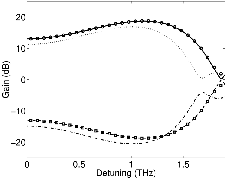
Fig. 1: Gain spectra vs. detuning for optimized PSAs made from (a) lossless fiber of length $L=3.63$ km and ${\rm Im}\{\gamma_{\Omega}\}=0$ (solid curve), (b) same as (a), but ${\rm Im}\{\gamma_{\Omega}\}$ calculated for DSF as explained in the text (circles), (c) $4.44$ km of DSF with $L_{\rm eff}=3.63$ km for $\alpha_{a}=\alpha_{s}=\alpha_{p}=0.41$ dB$/$km and ${\rm Im}\{\gamma_{\Omega}\}$ calculated for DSF as explained in the text (dotted curve). Gain spectra vs. detuning for optimized PSDs made from (d) lossless fiber of length $L=3.63$ km and ${\rm Im}\{\gamma_{\Omega}\}=0$ (dashed curve), (b) same as (a), but ${\rm Im}\{\gamma_{\Omega}\}$ calculated for DSF as explained in the text (squares), (c) $4.44$ km of DSF with $L_{\rm eff}=3.63$ km for $\alpha_{a}=\alpha_{s}=\alpha_{p}=0.41$ dB$/$km and ${\rm Im}\{\gamma_{\Omega}\}$ calculated for DSF as explained in the text (dash-dotted curve). Input pump power is $0.33$ Watts, $\lambda_{0}=1551.16$ nm, pump wavelength is $1551.5$ nm, and the dispersion slope is $57$ ps$/$(nm² km).

In Fig. 1 all of the plots are optimal in the sense that the best total phase and relative power of the input fields is chosen. It is clear that the Raman effect is negligible as those curves including the Raman effect (circles and squares) are very similar to those neglecting it (solid curve and dashed curve). This plot shows also that the definition of the effective length is a mathematical one and not a good guide for estimating the gain profile. The dotted and dash-dot curves show the gain spectrum of a lossy fiber ($0.41$ dB$/$km) $4.44$ km in length. The other curves are for a lossless fiber of effective length $L_{\rm eff}=3.63$ km. Thus distributed loss has a greater effect than might be supposed: fibers experience noticeably less gain than lossless fibers do when the lossless fiber has a length equal to the effective length of a lossy fiber.

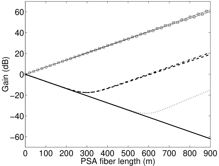
Fig. 2: Gain vs. fiber length for PSA made from DSF for (a) phase-sensitive deamplification with optimum power splitting in lossless fiber ($\alpha_{a}=\alpha_{s}=\alpha_{p}=0$) (thick solid line), (b) phase-sensitive deamplification with optimum power splitting in a lossy fiber ($\alpha_{a}=\alpha_{s}=\alpha_{p}=0.25$ dB$/$km) (dotted line), (c) phase-sensitive deamplification in a lossless fiber with $|\zeta_{a}|^{2}=|\zeta_{s}|^{2}$ (dash-dotted line), (d) phase-sensitive deamplification in a lossy fiber with $|\zeta_{a}|^{2}=|\zeta_{s}|^{2}$ (dashed line), (e) phase-sensitive amplification in a lossless fiber with $|\zeta_{a}|^{2}=|\zeta_{s}|^{2}$ (squares) and optimum input power splitting (solid curve under the squares), and (f) phase-sensitive amplification in a lossy fiber with $|\zeta_{a}|^{2}=|\zeta_{s}|^{2}$ (circles) and optimum input power splitting (solid curve under the circles). Input pump power is $4$ Watts, pump-signal detuning is $1$ THz, and phase-matching is achieved at the input [$\Delta k=-2{\rm Re}\{\gamma_{\Omega}\}I_{p}(0)$].

Some of the characteristics of the classical phase-sensitive response can be seen in Fig. 2, which is a plot of the phase-sensitive gain vs. fiber length. The primary feature of phase-sensitive amplification is that the mean-field gain is relatively insensitive to the relative strength of the two input fields (this can be seen by the overlap of the thin solid lines with the squares and circles). In addition, typical distributed losses do not significantly impact the gain of the fiber, as can be seen by comparison of the squares (lossless fiber) with the circles, which represent fiber with loss of $0.25$ dB$/$km. On the other hand, the achievable degree of phase-sensitive deamplification is much more sensitive to the relative proportion of the input fields which can be seen by comparison of the dash-dotted and dashed lines (equal power splitting, i.e., $|\zeta_{a}|^{2}=|\zeta_{s}|^{2}$) with the dotted and thick solid line (optimum relative proportion). In addition, distributed losses also set a limit on classical deamplification as can be seen by comparison of the dashed line (lossy) with the dash-dotted lines (lossless) and comparison of the dotted line (lossy) with the thick solid line (lossless).

3 Input-output quantum mode transformations

In this section, we discuss the quantum mechanics of the $\chi^{(3)}$ parametric amplifier with a strong, undepleted, coherent-state pump and derive input-output mode transformations in the Heisenberg picture which can be used to calculate the noise figure of the phase-sensitive operation of a FOPA and the accompanying quadrature squeezing. Here we also extend our previously described quantum theory[10, 11] to include the effects of loss. In order to make our treatment consistent with the customary formalism in quantum optics, we rescale our field to a photon-flux field, i.e. the expectation of the field $\langle\hat{A}\rangle=\bar{A}=A/\sqrt{\hbar\omega}$ so that $|\bar{A}|^{2}$ has units of photons/sec. We also rescale our nonlinear coefficient $\bar{\gamma}_{\Omega}=\gamma_{\Omega}\hbar\omega$, where $\hbar$ is Planck’s constant over $2\pi$.

We begin with the continuous-time quantum equation of motion for a multi-mode field in the presence of a non-instantaneous nonlinearity. This model was presented by Carter and Drummond [33, 38], solved for the case of dispersionless self-phase modulation by Boivin [31], and also derived in detail by Kärtner [32]. We have

$$\frac{\partial\hat{A}(t)}{\partial z} = -\int\frac{\alpha(\Omega)}{2}\widetilde{\hat{A}}(\Omega)\exp(-i\Omega t)\,{\rm d}\Omega+i\left[\int{\textrm{ d}}\tau\,{\bar{\gamma}}(t-\tau)\hat{A}^{\dagger}(\tau)\hat{A}(\tau)\right]\hat{A}(t)$$ (44)

$$+ i\,\hat{m}(z,t)\hat{A}(t){+\hat{l}(z,t)},$$

wherein ${\bar{\gamma}(t)}$ is the causal response function of the nonlinearity, i.e., the inverse Fourier transform of ${\bar{\gamma}_{\Omega}}$ in Eq. (4). In Eq. (44), $\hat{m}(z,t)$ is a Hermitian phase-noise operator

$${\hat{m}(z,t)=\int_{0}^{\infty}{\rm{d}}\Omega\,\,\frac{\sqrt{2{\rm Im}\{\bar{\gamma}_{\Omega}\}}}{{2\pi}}\{i\,\hat{d}^{\dagger}_{\Omega}(z)e^{i\,\Omega t}-i\,\hat{d}_{\Omega}(z)e^{-i\Omega t}\},}$$ (45)

which describes coupling of the field to a collection of localized, independent, medium oscillators (optical phonon modes). In addition, $\hat{l}(t)$ is a noise operator

$${\hat{l}(t)=\int_{-\infty}^{\infty}{\rm d}\Omega\frac{\sqrt{\alpha_{\Omega}}}{2\pi}\exp(i\Omega t)\hat{v}_{\Omega}(t)},$$ (46)

which describes the coupling of the field to a collection of localized, independent, oscillators in vacuum state. This coupling is required to preserve the continuous-time commutators

$$[\hat{A}(t),\hat{A}^{\dagger}(t^{\prime})]=\delta(t-t^{\prime}),$$ (47)

$$[\hat{A}(t),\hat{A}(t^{\prime})]=0.$$ (48)

Note that the time $t$ is in a reference frame traveling at group velocity $v_{g}$, i.e., $t=t_{\rm{stationary\,\,frame}}-\frac{z}{v_{g}}$. The weighting function ${\sqrt{2{\rm Im}\{\bar{\gamma}_{\Omega}\}}}$ must be positive for $\Omega>0$ so that the molecular vibration oscillators absorb energy from the mean fields rather than providing energy to the mean fields. The operators $\hat{d}_{\Omega}(z)$ and $\hat{d}^{\dagger}_{\Omega}(z)$ obey the commutation relation

$$[\hat{d}_{\Omega}(z),\hat{d}^{\dagger}_{\Omega^{\prime}}(z^{\prime})]=\delta(\Omega-\Omega^{\prime})\delta(z-z^{\prime})$$ (49)

and each phonon mode is in thermal equilibrium:

$$\langle\hat{d}^{\dagger}_{\Omega}(z)\hat{d}_{\Omega^{\prime}}(z^{\prime})\rangle=\delta(\Omega-\Omega^{\prime})\delta(z-z^{\prime})n_{\rm{th}}$$ (50)

with a mean phonon number $n_{\rm{th}}=[\exp(\hbar\Omega/kT)-1]^{-1}$. Here $\hbar$ is Planck’s constant over $2\pi$, $k$ is Boltzmann’s constant, and $T$ is the temperature. The operators corresponding to vacuum modes mixing into the Stokes and anti-Stokes frequencies, $\hat{v}_{\pm\Omega}$, obey the commutation relations

$$[\hat{v}_{\pm\Omega}(z),\hat{v}^{\dagger}_{\pm\Omega}(z)]=\delta(\pm\Omega-\pm\Omega^{\prime})\delta(z-z^{\prime})$$ (51)

and have no photons in them, i.e., $\langle\hat{v}^{\dagger}_{\pm\Omega}(z)\hat{v}_{\pm\Omega^{\prime}}(z^{\prime})\rangle=0$.

We assume that the total field present at the input of the fiber contains only a single-frequency pump, a Stokes field, and a symmetrically placed anti-Stokes field. The operators corresponding to these modes are

$$\hat{A}(t)=\hat{A}_{p}+\hat{A}_{s}\exp(i\Omega t)+\hat{A}_{a}\exp(-i\Omega t).$$ (52)

We do not need to consider other modes in the fiber when the pump is strong ($|\bar{A}_{p}|^{2}\gg|\bar{A}_{a}|^{2},|\bar{A}_{s}|^{2})$ and remains undepleted and the Stokes and anti-Stokes frequencies of interest are too weak to serve as pumps to other nonlinear processes. When this latter condition occurs, fluctuations from other higher order mixing modes are not coupled in. In addition, the vacuum modes at the input do not grow due to parametric fluorescence to become sufficiently strong to serve as pumps for nonlinear processes. This is because the input Stokes and anti-Stokes fields would saturate the pump long before this would happen. Thus the symmetric pairing of the Stokes and anti-Stokes fields of interest is justified and the pairs do not couple through the nonlinear process to other frequencies.

In order to obtain the coupled-wave equations for the three frequencies of interest, we insert Eq. (52) into Eq. (44), take the Fourier transform of the resulting equation, and separate into different frequencies. The resulting nonlinear quantum operator equations are:

$$\frac{{\rm d}\hat{A}_{p}}{{\rm d}z} = i\bar{\gamma}_{0}\hat{A}_{p}^{\dagger}\hat{A}_{p}\hat{A}_{p}+i[\bar{\gamma}_{0}+\bar{\gamma}_{\Omega}]\hat{A}_{s}^{\dagger}\hat{A}_{s}\hat{A}_{p}+i[\bar{\gamma}_{0}+\bar{\gamma}_{-\Omega}]\hat{A}_{a}^{\dagger}\hat{A}_{a}\hat{A}_{p}$$ (53)

$$+ i[\bar{\gamma}_{-\Omega}+\bar{\gamma}_{\Omega}]\hat{A}_{p}^{\dagger}\hat{A}_{s}\hat{A}_{a}\exp(i\Delta kz)-\sqrt{2{\rm Im}\{\bar{\gamma}_{\Omega}}\}\hat{A}_{a}\hat{d}^{\dagger}_{\Omega}(z)\exp(-i(k_{p}-k_{a})kz)$$

$$+\sqrt{2{\rm Im}\{\bar{\gamma}_{\Omega}}\}\hat{A}_{s}\hat{d}_{\Omega}(z)\exp(-i(k_{p}-k_{s})kz)+\sqrt{2{\rm Im}\{\gamma_{\Omega\rightarrow 0}\}}\hat{A}_{p}[\hat{d}_{\Omega\rightarrow 0+}(z)+\hat{d}^{\dagger}_{\Omega\rightarrow 0-}(z)]$$

$$- \frac{\alpha_{p}}{2}\hat{A}_{p}+\sqrt{\alpha_{p}}\hat{v}_{p}(z),$$

$$\frac{{\rm d}\hat{A}_{a}}{{\rm d}z} = i[\bar{\gamma}_{0}+\bar{\gamma}_{\Omega}]\hat{A}_{p}^{\dagger}\hat{A}_{p}\hat{A}_{a}+i\bar{\gamma}_{0}\hat{A}_{a}^{\dagger}\hat{A}_{a}\hat{A}_{a}+i[\bar{\gamma}_{0}+\bar{\gamma}_{2\Omega}]\hat{A}_{s}^{\dagger}\hat{A}_{s}\hat{A}_{a}$$ (54)

$$+ i\bar{\gamma}_{\Omega}\hat{A}_{p}^{2}\hat{A}_{s}^{\dagger}\exp(-i\Delta kz)-\sqrt{2{\rm Im}\{\bar{\gamma}_{\Omega}}\}\hat{A}_{p}\exp[i(k_{p}-k_{a})z]\hat{d}_{\Omega}(z)$$

$$- \frac{\alpha_{a}}{2}\hat{A}_{a}+\sqrt{\alpha_{a}}\hat{v}_{a}(z),$$

$$\frac{{\rm d}\hat{A}_{s}}{{\rm d}z} = i[\bar{\gamma}_{0}+\bar{\gamma}_{-\Omega}]\hat{A}_{p}^{\dagger}\hat{A}_{p}\hat{A}_{s}+i\bar{\gamma}_{0}\hat{A}_{s}^{\dagger}\hat{A}_{s}\hat{A}_{s}+i[\bar{\gamma}_{0}+\bar{\gamma}_{-2\Omega}]\hat{A}_{a}^{\dagger}\hat{A}_{a}\hat{A}_{s}$$ (55)

$$+ i\bar{\gamma}_{-\Omega}\hat{A}_{p}^{2}\hat{A}_{a}^{\dagger}\exp(-i\Delta kz)+\sqrt{2{\rm Im}\{\bar{\gamma}_{\Omega}}\}\hat{A}_{p}\exp[i(k_{p}-k_{s})z]\hat{d}_{\Omega}^{\dagger}(z)$$

$$- \frac{\alpha_{s}}{2}\hat{A}_{s}+\sqrt{\alpha_{s}}\hat{v}_{s}(z).$$

Eqs. (53 - 55) are nonlinear in the quantum operators (except for the last two terms of each equation) and are difficult to solve. However, one may linearize these equations around the mean values of the operators and obtain solutions accurate to first order in the fluctuations. Using the definition

$$\hat{A}_{j}=\bar{A}_{j}+\hat{a}_{j},$$ (56)

where $\bar{A}_{j}$ represents a c-number mean value of $\hat{A}_{j}$ and $\hat{a}_{j}$ represents the quantum fluctuations of $\hat{A}_{j}$, and where $j=p,a,s$, we expand Eqs. (53 - 55) to obtain the following equations for the mean values (i.e., those terms containing no fluctuation operators):

$$\frac{{\rm d}\bar{A}_{p}}{{\rm d}z} = i\bar{\gamma}_{0}\bar{A}_{p}^{*}\bar{A}_{p}\bar{A}_{p}+i[\bar{\gamma}_{0}+\bar{\gamma}_{\Omega}]\bar{A}_{s}^{*}\bar{A}_{s}\bar{A}_{p}+i[\bar{\gamma}_{0}+\bar{\gamma}_{-\Omega}]\bar{A}_{a}^{*}\bar{A}_{a}\bar{A}_{p}$$ (57)

$$+i[\bar{\gamma}_{-\Omega}+\bar{\gamma}_{\Omega}]\bar{A}_{p}^{*}\bar{A}_{s}\bar{A}_{a}\exp(i\Delta kz)-\frac{\alpha_{p}}{2}\bar{A}_{p},$$

$$\frac{{\rm d}\bar{A}_{a}}{{\rm d}z} = i[\bar{\gamma}_{0}+\bar{\gamma}_{\Omega}]\bar{A}_{p}^{*}\bar{A}_{p}\bar{A}_{a}+i\bar{\gamma}_{0}\bar{A}_{a}^{*}\bar{A}_{a}\bar{A}_{a}+i[\bar{\gamma}_{0}+\bar{\gamma}_{2\Omega}]\bar{A}_{s}^{*}\bar{A}_{s}\bar{A}_{a}$$ (58)

$$+i\bar{\gamma}_{\Omega}\bar{A}_{p}^{2}\bar{A}_{s}^{*}\exp(-i\Delta kz)-\frac{\alpha_{a}}{2},\bar{A}_{a}$$

$$\frac{{\rm d}\bar{A}_{s}}{{\rm d}z} = i[\bar{\gamma}_{0}+\bar{\gamma}_{-\Omega}]\bar{A}_{p}^{*}\bar{A}_{p}\bar{A}_{s}+i\bar{\gamma}_{0}\bar{A}_{s}^{*}\bar{A}_{s}\bar{A}_{s}+i[\bar{\gamma}_{0}+\bar{\gamma}_{-2\Omega}]\bar{A}_{a}^{*}\bar{A}_{a}\bar{A}_{s}$$ (59)

$$+i\bar{\gamma}_{-\Omega}\bar{A}_{p}^{2}\bar{A}_{a}^{*}\exp(-i\Delta kz)-\frac{\alpha_{s}}{2}\bar{A}_{s}.$$

The equations for those terms which contain one fluctuation operator are

$$\frac{{\rm d}\hat{a}_{p}}{{\rm d}z} = i\bar{\gamma}_{0}[2|\bar{A}_{p}|^{2}\hat{a}_{p}+\bar{A}_{p}^{2}\hat{a}_{p}^{\dagger}]+i[\bar{\gamma}_{0}+\bar{\gamma}_{\Omega}][|\bar{A}_{s}|^{2}\hat{a}_{p}+\bar{A}_{s}^{*}\bar{A}_{p}\hat{a}_{s}+\bar{A}_{s}\bar{A}_{p}\hat{a}_{s}^{\dagger}]$$ (60)

$$+i[\bar{\gamma}_{0}+\bar{\gamma}_{-\Omega}][|\bar{A}_{a}|^{2}\hat{a}_{p}+\bar{A}_{a}^{*}\bar{A}_{p}\hat{a}_{a}+\bar{A}_{a}\bar{A}_{p}\hat{a}_{a}^{\dagger}]$$

$$+i[\bar{\gamma}_{-\Omega}+\bar{\gamma}_{\Omega}][\bar{A}_{p}^{*}\bar{A}_{s}\hat{a}_{a}+\bar{A}_{p}^{*}\bar{A}_{a}\hat{a}_{s}+\bar{A}_{s}\bar{A}_{a}\hat{a}_{p}^{\dagger}]\exp(i\Delta kz)$$

$$-\sqrt{2{\rm Im}\{\bar{\gamma}_{\Omega}}\}\bar{A}_{a}\hat{d}^{\dagger}_{\Omega}(z)\exp(-i(k_{p}-k_{a})kz)+\sqrt{2{\rm Im}\{\bar{\gamma}_{\Omega}}\}\bar{A}_{s}\hat{d}_{\Omega}(z)\exp(-i(k_{p}-k_{s})kz)$$

$$+\sqrt{2{\rm Im}\{\gamma_{\Omega\rightarrow 0}\}}\bar{A}_{p}[\hat{d}_{\Omega\rightarrow 0+}(z)+\hat{d}^{\dagger}_{\Omega\rightarrow 0-}(z)]-\frac{\alpha_{p}}{2}\hat{a}_{p}+\sqrt{\alpha_{p}}\hat{v}_{p}(z),$$

$$\frac{{\rm d}\hat{a}_{a}}{{\rm d}z} = i[\bar{\gamma}_{0}+\bar{\gamma}_{\Omega}][|\bar{A}_{p}|^{2}\hat{a}_{a}+\bar{A}_{p}^{*}\bar{A}_{a}\hat{a}_{p}+\bar{A}_{p}\bar{A}_{a}\hat{a}_{p}^{\dagger}]+i\bar{\gamma}_{0}[2|\bar{A}_{a}|^{2}\hat{a}_{a}+\bar{A}_{a}^{2}\hat{a}_{a}^{\dagger}]$$ (61)

$$+i[\bar{\gamma}_{0}+\bar{\gamma}_{2\Omega}][|\bar{A}_{s}|^{2}\hat{a}_{a}+\bar{A}_{s}^{*}\bar{A}_{a}\hat{a}_{s}+\bar{A}_{s}\bar{A}_{a}\hat{a}_{s}^{\dagger}]+i\bar{\gamma}_{\Omega}[\bar{A}_{p}^{2}\hat{a}_{s}^{\dagger}+2\bar{A}_{p}\bar{A}_{s}^{*}\hat{a}_{p}]\exp(-i\Delta kz)$$

$$+\sqrt{2{\rm Im}\{\bar{\gamma}_{\Omega}}\}\hat{A}_{p}\exp[i(k_{p}-k_{a})z]\hat{d}_{\Omega}(z)-\frac{\alpha_{a}}{2}\hat{a}_{a}+\sqrt{\alpha_{a}}\hat{v}_{a}(z),$$

$$\frac{{\rm d}\hat{a}_{s}}{{\rm d}z} = i[\bar{\gamma}_{0}+\bar{\gamma}_{-\Omega}][|\bar{A}_{p}|^{2}\hat{a}_{s}+\bar{A}_{p}^{*}\bar{A}_{s}\hat{a}_{p}+\bar{A}_{p}\bar{A}_{s}\hat{a}_{p}^{\dagger}]+i\bar{\gamma}_{0}[2|\bar{A}_{s}|^{2}\hat{a}_{s}+\bar{A}_{s}^{2}\hat{a}_{s}^{\dagger}]$$ (62)

$$+i[\bar{\gamma}_{0}+\bar{\gamma}_{-2\Omega}][|\bar{A}_{a}|^{2}\hat{a}_{s}+\bar{A}_{a}^{*}\bar{A}_{s}\hat{a}_{a}+\bar{A}_{a}\bar{A}_{s}\hat{a}_{a}^{\dagger}]+i\bar{\gamma}_{-\Omega}[\bar{A}_{p}^{2}\hat{a}_{a}^{\dagger}+2\bar{A}_{p}\bar{A}_{a}^{*}\hat{a}_{p}]\exp(-i\Delta kz)$$

$$-\sqrt{2{\rm Im}\{\bar{\gamma}_{\Omega}}\}\hat{A}_{p}\exp[i(k_{p}-k_{s})z]\hat{d}_{\Omega}^{\dagger}(z)-\frac{\alpha_{s}}{2}\hat{a}_{s}+\sqrt{\alpha_{s}}\hat{v}_{s}(z).$$

When the amplifier is operating in the unsaturated regime, the pump is depleted to a negligible degree. Thus one may neglect the four wave-mixing terms in Eq. (57). We next make the strong pump approximation, i.e., $|\bar{A}_{p}|^{2}\gg|\bar{A}_{a}|^{2},|\bar{A}_{s}|^{2}$ , which is valid at the input of the fiber under typically used operating conditions and remains valid when there is essentially no pump depletion. Under these conditions, we note that the cross-phase modulation of the pump wave due to the Stokes and anti-Stokes fields is negligible. We thus obtain the final form of the mean-field equations:

$$\frac{{\rm{d}}\bar{A}_{p}}{{\rm{d}}z} = i\,\bar{\gamma}_{0}\,|\bar{A}_{p}|^{2}\bar{A}_{p}-\frac{\alpha_{p}}{2}\bar{A}_{p},$$ (63)

$$\frac{{\rm{d}}\bar{A}_{a}}{{\rm{d}}z} = i\,(\bar{\gamma}_{0}+\bar{\gamma}_{\Omega})\,|\bar{A}_{p}|^{2}\bar{A}_{a}+i\bar{\gamma}_{\Omega}\bar{A}_{p}^{2}\bar{A}_{s}^{*}\exp{(-i\Delta kz)}-\frac{\alpha_{a}}{2}\bar{A}_{a},$$ (64)

$$\frac{{\rm{d}}\bar{A}_{s}}{{\rm{d}}z} = i\,(\bar{\gamma}_{0}+\bar{\gamma}_{-\Omega})\,|\bar{A}_{p}|^{2}\bar{A}_{s}+i\bar{\gamma}_{-\Omega}\bar{A}_{p}^{2}\bar{A}_{a}^{*}\exp{(-i\Delta kz)}-\frac{\alpha_{s}}{2}\bar{A}_{s}.$$ (65)

The solution of these mean-field equations [Eqs. (7-9)] were examined in the previous section. Examining the fluctuation equations, we note that the first-order fluctuation equations [Eqs. (60-62)] are linear in their quantum operators. The higher-order fluctuation terms are nonlinear in the quantum-fluctuation operators, but their contribution is negligible because they cannot contain terms proportional to $\bar{A}_{p}^{2}$. We thus neglect the higher-order fluctuation equations which are not reported here.

Similarly, those fluctuation terms in Eqs. (60-62) that do not contain two pump factors can be neglected, as they are much weaker than the other terms. We remark here that the Langevin-noise terms due to the Raman effect in Eqs. (61-62) will not be neglected. This is justified because comparison of the amplitude of the Langevin terms, $\sqrt{2{\rm Im}\{\bar{\gamma}_{\Omega}}\}\hat{A}_{p}$, in Eqs. (61-62) with the the amplitude of those four-wave-mixing terms in Eqs. (61-62) that contain only one pump term, for example $\bar{\gamma}_{-\Omega}\bar{A}_{p}\bar{A}_{a}^{*}\hat{a}_{p}$ shows that the Langevin term is much greater than the one-pump-field four-wave-mixing terms. For example, consider the symmetrized magnitude of the two terms:

$$\sqrt{\frac{2{\rm Im}\{\bar{\gamma}_{-\Omega}\}|\bar{A}_{p}|^{2}[\langle\hat{d}^{\dagger}_{\Omega}\hat{d}_{\Omega}+\hat{d}_{\Omega}\hat{d}^{\dagger}_{\Omega}\rangle]/2}{4\bar{\gamma}_{-\Omega}^{2}|\bar{A}_{a}|^{2}|\bar{A}_{p}|^{2}[\langle\hat{a}_{p}^{\dagger}\hat{a}_{p}+\hat{a}_{p}\hat{a}_{p}^{\dagger}\rangle]/2}}=\sqrt{\frac{{\rm Im}\{\bar{\gamma}_{-\Omega}\}(n_{\rm{th}}+1)}{2|\bar{\gamma}_{-\Omega}|^{2}\langle\hat{n}_{a}\rangle}}.$$ (66)

For an anti-Stokes amplitude of up to 10 mW (a flux of $\hat{n}_{a}=7.8\times 10^{16}$ photons/s ) this ratio is greater than 25 for pure silica and even better for materials with stronger Raman gains (such as dispersion-shifted and highly nonlinear fibers). This means that the Langevin noise term should be included.

One last simplification can be made to the pump equation, Eq. (60). We simply note that all of the remaining noise terms in Eq. (60) affect only the pump field and that under the undepleted, strong-pump approximation, the Stokes and anti-Stokes fields do not interact with the pump fluctuations to first degree. This is the case if one assumes that the pump is, or nearly is, in a coherent state. Thus, as we are only interested in the noise introduced during the amplification process to the Stokes and anti-Stokes fields, we neglect the pump fluctuations and replace Eq. (60) with

$$\frac{{\rm d}\hat{a}_{p}}{{\rm d}z}=0.$$ (67)

This allows one to treat the pump field fully classically. To summarize the steps taken, the undepleted, strong, coherent-state pump approximation yields the following equations for the first-order fluctuations:

$$\frac{{\rm d}\hat{a}_{a}}{{\rm d}z} = i[\bar{\gamma}_{0}+\bar{\gamma}_{\Omega}]|\bar{A}_{p}|^{2}\hat{a}_{a}+i\bar{\gamma}_{\Omega}\bar{A}_{p}^{2}\hat{a}_{s}^{\dagger}\exp(-i\Delta kz)$$ (68)

$$+\sqrt{2{\rm Im}\{\bar{\gamma}_{\Omega}}\}\hat{A}_{p}\exp[i(k_{p}-k_{a})z]\hat{d}_{\Omega}(z)-\frac{\alpha_{a}}{2}\hat{a}_{a}+\sqrt{\alpha_{a}}\hat{v}_{a}(z),$$

$$\frac{{\rm d}\hat{a}_{s}}{{\rm d}z} = i[\bar{\gamma}_{0}+\bar{\gamma}_{-\Omega}]|\bar{A}_{p}|^{2}\hat{a}_{s}+i\bar{\gamma}_{-\Omega}\bar{A}_{p}^{2}\hat{a}_{a}^{\dagger}\exp(-i\Delta kz)$$ (69)

$$-\sqrt{2{\rm Im}\{\bar{\gamma}_{\Omega}}\}\hat{A}_{p}\exp[i(k_{p}-k_{s})z]\hat{d}_{\Omega}^{\dagger}(z)-\frac{\alpha_{s}}{2}\hat{a}_{s}+\sqrt{\alpha_{s}}\hat{v}_{s}(z).$$

We note that Eqs. (67-69) can be combined with Eqs. (63-65) by using Eq. (56) to yield:

$$\frac{{\rm{d}}\bar{A}_{p}}{{\rm{d}}z} = i\,\bar{\gamma}_{0}\,|\bar{A}_{p}|^{2}\bar{A}_{p}-\frac{\alpha_{p}}{2}\bar{A}_{p},$$ (70)

$$\frac{{\rm{d}}\hat{A}_{a}}{{\rm{d}}z} = i\,(\bar{\gamma}_{0}+\bar{\gamma}_{\Omega})\,|\bar{A}_{p}|^{2}\hat{A}_{a}+i\bar{\gamma}_{\Omega}\bar{A}_{p}^{2}\hat{A}_{s}^{\dagger}\exp{(-i\Delta kz)}-\frac{\alpha_{a}}{2}\hat{A}_{a}$$ (71)

$$+\sqrt{2{\rm Im}\{\bar{\gamma}_{\Omega}\}}\bar{A}_{p}\exp[i(k_{p}-k_{a})z]\hat{d}_{\Omega}(z)+\sqrt{\alpha_{a}}\hat{v}_{a}(z),$$

$$\frac{{\rm{d}}\hat{A}_{s}}{{\rm{d}}z} = i\,(\bar{\gamma}_{0}+\bar{\gamma}_{-\Omega})\,|\bar{A}_{p}|^{2}\hat{A}_{s}+i\bar{\gamma}_{-\Omega}\bar{A}_{p}^{2}\hat{A}_{a}^{\dagger}\exp{(-i\Delta kz)}-\frac{\alpha_{s}}{2}\hat{A}_{s}$$ (72)

$$-\sqrt{2{\rm Im}\{\bar{\gamma}_{\Omega}\}}\bar{A}_{p}\exp[i(k_{p}-k_{s})z]\hat{d}_{\Omega}^{\dagger}(z)+\sqrt{\alpha_{s}}\hat{v}_{s}(z).$$

This final form of the equations allows one to evolve the mean fields of all three frequencies and the fluctuations of the Stokes and anti-Stokes wavelengths simultaneously.

The solution of Eqs. (71) and (72) is

$$\hat{A}_{a}(L) = \mu_{a}(0,L)\hat{A}_{a}(0)+\nu_{a}(0,L)\hat{A}_{s}^{\dagger}(0)+$$ (73)

$$\sqrt{2{\rm Im}\{\bar{\gamma}_{\Omega}\}}\int_{0}^{L}{\rm d}z\,\bar{A}_{p}(z)\exp[i(k_{p}-k_{a})z]\left[\mu_{a}(z,L)-\nu_{a}(z,L)\right]\hat{d}_{\Omega}(z),$$

$$+\int_{0}^{L}{\rm d}z\,[\sqrt{\alpha_{a}}\mu_{a}(z,L)\hat{v}_{a}(z)+\sqrt{\alpha_{s}}\nu_{a}(z,L)\hat{v}_{s}^{\dagger}(z)]$$

$$\hat{A}_{s}(L) = \mu_{s}(0,L)\hat{A}_{s}(0)+\nu_{s}(0,L)\hat{A}_{a}^{\dagger}(0)+$$ (74)

$$\sqrt{2{\rm Im}\{\bar{\gamma}_{\Omega}\}}\int_{0}^{L}{\rm d}z\,\bar{A}_{p}(z)\exp[i(k_{p}-k_{s})z]\left[-\mu_{s}(z,L)+\nu_{s}(z,L)\right]\hat{d}_{\Omega}^{\dagger}(z).$$

$$+\int_{0}^{L}{\rm d}z\,[\sqrt{\alpha_{s}}\mu_{s}(z,L)\hat{v}_{s}(z)+\sqrt{\alpha_{a}}\nu_{s}(z,L)\hat{v}_{a}^{\dagger}(z)]$$

In the notation used in this paper, the functions $\mu_{j}(z,L)$ and $\nu_{j}(L,z)$ denote evolution from a point $z$ in the fiber to the end of the fiber ($L$) where the intensity and phase of the pump at point $z$ must be used.

In this section, we have presented a thorough derivation of the input-output mode transformations that govern a $\chi^{(3)}$ parametric amplifier. In the following two sections, we use these input-output mode transformations to obtain the noise figure of $\chi^{(3)}$ phase-sensitive parametric amplifiers and the squeezing parameter for quadrature squeezing.

4 Noise Figure of phase-sensitive amplification

In this section we discuss the noise figure of phase-sensitive amplification, which is defined as

$${\rm NF}=\frac{{\rm SNR}_{\rm in}}{{\rm SNR}_{\rm out}}.$$ (75)

We assume for our treatment here that the difference between the Stokes and anti-Stokes frequencies exceeds the bandwidth of the detector. Thus beat frequencies of these two waves will not be detected and can be neglected. The mean photon flux at the Stokes and anti-Stokes wavelength is $\langle\hat{n}_{j}\rangle=\langle\hat{A}_{j}^{\dagger}(0)\hat{A}_{j}(0)\rangle=|\zeta_{j}|^{2}$, and is assumed to be in a coherent state. In what follows, we neglect the small frequency difference between $\omega_{a}$ and $\omega_{s}$. Thus the input SNR can be written as

$${\rm SNR}_{\rm in}=\frac{(\langle\hat{n}_{a}\rangle+\langle\hat{n}_{s}\rangle)^{2}}{\langle\Delta\hat{n}^{2}_{a}\rangle+\langle\Delta\hat{n}^{2}_{s}\rangle}=\frac{(|\zeta_{a}|^{2}+|\zeta_{s}|^{2})^{2}}{|\zeta_{a}|^{2}+|\zeta_{s}|^{2}}=|\zeta_{a}|^{2}+|\zeta_{s}|^{2}.$$ (76)

Calculating the output SNR in a similar way and plugging into Eq. (75), the NF for phase-sensitive amplification can be expressed as

$${\rm NF}=\frac{(|\zeta_{a}|^{2}+|\zeta_{s}|^{2})(\langle\Delta\hat{n}^{2}_{\rm PI}\rangle+\langle\Delta\hat{n}^{2}_{\rm PS}\rangle)}{(P_{a}+P_{s})^{2}},$$ (77)

where the mean output power at each wavelength, $P_{a}$ and $P_{s}$, is

$$P_{a} = |\mu_{a}|^{2}|\zeta_{a}|^{2}+|\nu_{a}|^{2}|\zeta_{s}|^{2}+(\zeta_{a}\zeta_{s}\mu_{a}\nu_{a}^{*}+{\rm c.c.}),$$ (78)

$$P_{s} = |\mu_{s}|^{2}|\zeta_{s}|^{2}+|\nu_{s}|^{2}|\zeta_{a}|^{2}+(\zeta_{a}\zeta_{s}\mu_{s}\nu_{s}^{*}+{\rm c.c.}).$$ (79)

In Eq. (77), we have expressed the variance of the output photocurrent as the sum of a phase-insensitive portion, $\langle\Delta\hat{n}^{2}_{\rm PI}\rangle$, and a phase-sensitive portion, $\langle\Delta\hat{n}^{2}_{\rm PS}\rangle$, which are calculated to be

$$\langle\Delta\hat{n}^{2}_{\rm PI}\rangle = P_{a}B_{a}+P_{s}B_{s},$$ (80)

$$\langle\Delta\hat{n}^{2}_{\rm PS}\rangle = 2Q^{*}B_{1}+2QB_{2},$$ (81)

where the quantities

$$B_{j} = |\mu_{j}|^{2}+|\nu_{j}|^{2}+(2n_{\rm{th}}+1)|r_{j}|^{2}+|c_{j1}|^{2}+|c_{j2}|^{2},\,\,\,(j=a,s)$$ (82)

$$Q = (\mu_{a}\zeta_{a}+\nu_{a}\zeta_{s}^{*})(\mu_{s}\zeta_{s}+\nu_{s}\zeta_{a}^{*}),$$ (83)

$$B_{1} = c_{x1}+r_{x}(n_{\rm{th}}+1)+\mu_{a}\nu_{s},$$ (84)

$$B_{2} = c_{x2}^{*}+r_{x}^{*}n_{\rm{th}}+\mu_{s}^{*}\nu_{a}^{*},$$ (85)

have noise terms defined as follows:

$$|r_{a}|^{2} = 2{\rm Im}\{\bar{\gamma}_{\Omega}\}\int_{0}^{L}{\rm d}z\,|\bar{A}_{p}(z)|^{2}|\mu_{a}(z,L)-\nu_{a}(z,L)|^{2},$$ (86)

$$|r_{s}|^{2} = -2{\rm Im}\{\bar{\gamma}_{-\Omega}\}\int_{0}^{L}{\rm d}z\,|\bar{A}_{p}(z)|^{2}|\mu_{s}(z,L)-\nu_{s}(z,L)|^{2},$$ (87)

$$|c_{a(s)1}|^{2} = \int_{0}^{L}{\rm d}z\,\alpha_{a(s)}|\mu_{a(s)}(z,L)|^{2},$$ (88)

$$|c_{a(s)2}|^{2} = \int_{0}^{L}{\rm d}z\,\alpha_{s(a)}|\nu_{a(s)}(z,L)|^{2},$$ (89)

$$r_{x} = 2{\rm Im}\{\bar{\gamma}_{\Omega}\}\int_{0}^{L}{\rm d}z\,\bar{A}_{p}^{2}(z)\exp(-i\Delta kz)$$ (90)

$$\times[\mu_{a}(z,L)-\nu_{a}(z,L)][-\mu_{s}(z,L)+\nu_{s}(z,L)],$$

$$c_{x1} = \alpha_{a}\int_{0}^{L}{\rm d}z\,\mu_{a}(z,L)\nu_{s}(z,L),$$ (91)

$$c_{x2}^{*} = \alpha_{s}\int_{0}^{L}{\rm d}z\,\nu_{a}(z,L)^{*}\mu_{s}(z,L)^{*}.$$ (92)

In the above expressions, $|r_{a(s)}|^{2}$ represents the integrated amplified noise at the anti-Stokes (Stokes) wavelength seeded by thermally populated optical phonon modes that are coupled in by the Raman process. The terms $|c_{a(s)1}|^{2}$ represent integrated amplified noise at the anti-Stokes (Stokes) wavelength seeded by vacuum noise mixed in through distributed loss at the anti-Stokes (Stokes) wavelength, while the terms $|c_{a(s)2}|^{2}$ represent amplified noise at the anti-Stokes (Stokes) wavelength seeded by vacuum noise mixed in through distributed loss at the Stokes (anti-Stokes) wavelength.

In addition, the phase-sensitive terms $\mu_{a}\nu_{s}$ and $\mu_{s}^{*}\nu_{a}^{*}$ represent amplified phase-sensitive noise seeded by the vacuum noise at the anti-Stokes and Stokes wavelengths. The quantity $r_{x}$ represents amplified phase-sensitive noise seeded by the thermal-phonon fields due the Raman effect, and $c_{x1}$ and $c_{x2}$ represent the amplified phase-sensitive noise seeded by the vacuum noise due to distributed linear losses. Phase-sensitive noise is present when the photocurrent variance with both Stokes and anti-Stokes waves impinging on a detector is different from the sum of the individual noise variances of the Stokes and anti-Stokes frequencies.

4.A Degenerate Limit

By taking the limiting value of the NF as $\Omega\rightarrow 0$, we find the NF performance of a fully degenerate FOPA. We find this limiting value of the NF by expanding the anti-symmetric imaginary part of $\bar{\gamma}_{\Omega}$ in a Taylor seris and expanding the exponential in $n_{th}=\{\exp[\hbar\Omega/(kT)]-1\}^{-1}$ before allowing $\Omega\rightarrow 0$. We also use the fact that in this limit, $\Delta k$ also approaches $0$ and the optimum power splitting ratio approaches $0.5$. This NF limit is:

$${\rm NF}_{\rm PSA,\,\Omega\rightarrow 0}=1+\frac{\frac{4kT\bar{\gamma}_{i}^{{}^{\prime}}(0)}{\hbar\bar{\gamma}_{0}}\left[1-\frac{\phi_{\rm NL}}{\sqrt{1+\phi_{\rm NL}^{2}}}\right]}{1+2\phi_{\rm NL}^{2}+2\phi_{\rm NL}\sqrt{1+\phi_{\rm NL}^{2}}},$$ (93)

where $\phi_{\rm NL}=\bar{\gamma}_{0}|\bar{A}_{p}|^{2}L$ is the nonlinear phase shift and $\bar{\gamma}_{i}^{{}^{\prime}}(0)$ is the slope of the imaginary part of $\bar{\gamma}_{\Omega}$ as $\Omega\rightarrow 0$. We observe that the PSA noise figure for $\Omega\rightarrow 0$ increases to a maximum of slightly more than $0$ dB and then decreases again and approaches $0$ dB in the high-gain limit. This unusual behaviour of decreasing noise figure vs. nonlinear phase shift is due to the relative scaling of the Raman and FWM processes when $\Delta k=0$ and fact that the mean Raman gain of the Stokes and anti-Stokes frequencies vanishes. The total Raman noise scales linearly whereas the two-frequency signal undergoes quadratic gain. Consequently, the Raman noise being created at the Stokes and anti-Stokes frequencies does not grow.

4.B Results

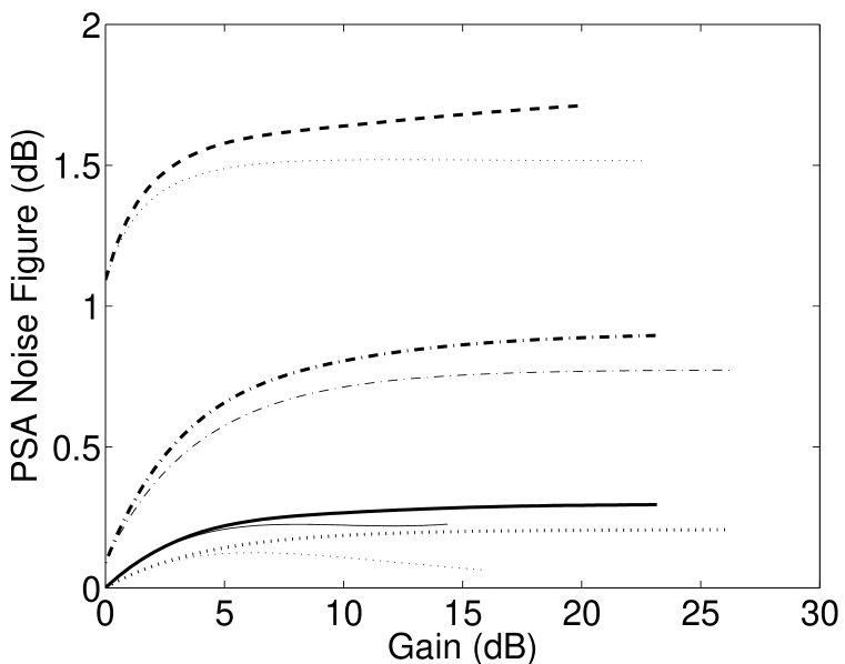
Fig. 3: PSA noise figure vs. gain for various detunings for a highly-nonlinear fiber. For thick lines, fiber attenuation is $0.75$ dB/km at pump, Stokes, and anti-Stokes wavelengths; for thin lines, fiber is lossless. $\Omega/2\pi=13.8$ THz, dashed curves; $\Omega/2\pi=1.38$ THz, dash-dotted curves; $\Omega/2\pi=40$ GHz, solid curves; and $\Omega/2\pi=0$ Hz, dotted curves. Except for dotted curves, phase matching at the input [$\Delta k=-2{\rm Re}\{\gamma_{\Omega}\}I_{p}(0)$] is achieved. For dotted curves, $\Delta k=0$. The anti-Stokes/Stokes relative phase and power splitting at the input is for optimal classical gain. Initial pump power is $340$ mW, $\gamma(0)=9\times 10^{-3}$ W^-1m^-1, peak imaginary part of $\gamma_{\Omega}$ is $3.5\times 10^{-3}$ W^-1m^-1. Fiber length is $1$ km.

In Fig. 3, we plot the noise figure vs. PSA gain for several values of detuning for a typical highly-nonlinear fiber with a loss coefficient corresponding to $0.75$ dB$/$km. The plots show that for detunings achievable by use of electrooptic elements (40 GHz detuning, phase-matched, solid curve), the results are almost exactly the same as would be achieved in the limit of zero detuning ( dotted). For these simulations, we use realistic values for $\bar{\gamma}(0)$ and for the distributed loss. We have additionally assumed that the highly-nonlinear fiber has the same ratio of ${\rm Im}\{\bar{\gamma}(\Omega)\}$ to ${\rm Re}\{\bar{\gamma}(\Omega)\}$ as the standard dispersion-shifted fiber, i.e., the two have the same germanium content. Unsurprisingly, we see by comparing the thick curves (lossy) to thin curves (lossless), that the distributed loss increases the noise figure. We aslo see that as the Raman-gain coefficient decreases, the noise figure improves.

Interestingly, unlike the PIA case, Fig. 3 shows that the PSA noise figure is greater than $0$ dB as the gain approaches $0$ dB. This occurs because the Raman gain and loss processes dominate in the early parts of the amplifier (Raman gain and loss are linear in the early parts of the amplifier while the four-wave-mixing gain is quadratic), adding noise to both frequencies, while the mean field undergoes no net gain due to the Raman loss at one frequency and the Raman gain at the other.

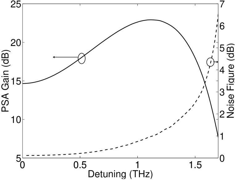
Fig. 4: PSA gain and noise-figure spectrum vs. detuning. Anti-Stokes/Stokes relative phase and input-power splitting is for optimal classical gain. Initial pump power is $300$ mW, $\gamma_{0}=2\times 10^{-3}$ W^-1m^-1, peak imaginary part of $\gamma_{\Omega}$ is $0.75\times 10^{-3}$ W^-1m^-1. Attenuation is $0.41$ dB/km at the pump, Stokes, and anti-Stokes wavelengths. Fiber length is $4$ km. $\lambda_{0}=1551.15$ nm, $\lambda_{p}=1555.5$ nm, and the dispersion slope is $57$ ps$/$nm$/$km²

In Fig. 4, we show the gain and noise-figure spectrum for a $4$ km fiber with fiber parameters as described in the caption. This plot shows that the increasing Raman-gain coefficient with detuning causes an increasing noise figure. These results show that for realistic optical fibers, a FOPA operated as a PSA can achieve a noise figure below $1$ dB for detunings up to $1$ THz.

5 Nondegenerate quadrature squeezing

When no light is injected into the FOPA, the quantum correlations between the Stokes and anti-Stokes modes imply the presence of quadrature squeezing, which is measurable by homodyne detection with a two-frequency local oscillator (LO).

The difference current of the homodyne detector may be written as

$$\hat{I}=\hat{b}^{\dagger}_{a}\hat{q}_{a}+\hat{b}^{\dagger}_{s}\hat{q}_{s}+{\rm H.c.},$$ (94)

where H.c. stands for the Hermitian conjugate of the first two terms; $\hat{q}_{a}$ and $\hat{q}_{s}$ are the annihilation operators corresponding to the anti-Stokes and Stokes components of the LO beams, which are in a coherent state each with photon flux $|\alpha_{{\rm LO},j}|^{2}$, relative intensity

$$y_{j}=\frac{|\alpha_{{\rm LO},j}|^{2}}{|\alpha_{{\rm LO},a}|^{2}+|\alpha_{{\rm LO},s}|^{2}},$$ (95)

and phase $\theta_{j}$ for $j=a,s$.

The squeezing parameter is defined as the ratio of the photocurrent variance with the pump on to the photocurrent variance with vacuum input to the homodyne detector (i.e., pump off).

5.A Lossless fiber with Raman effect

In this paper, we concentrate on squezzing results for a lossless FOPA. This is because increased nonlinear drive will, theoretically at least, overpower linear loss, leading to no hard limit on the achievable squeezing. However, as the Raman effect at each $z$ scales with pump intensity as does the four-wave-mixing process, the lossless case illustrates a fundamental limit on the achievable squeezing. Using Eqs. (94) and (95), we obtain, after some simple algebra, for the lossless Raman-active case:

$$S = \frac{\langle\Delta\hat{I}^{2}\rangle}{\langle\Delta\hat{I}^{2}\rangle_{\rm vac}}$$ (96)

$$= [1+2(|\nu_{a}|^{2}+|r_{a}|^{2}n_{\rm{th}})]y_{a}+\{1+2[|\nu_{s}|^{2}+|r_{s}|^{2}(1+n_{\rm{th}})]\}y_{s}$$

$$+2\{[\mu_{s}\nu_{a}(1+n_{\rm{th}})-\mu_{a}\nu_{s}n_{\rm{th}}]\exp[-i(\theta_{a}+\theta_{s})]+{\rm c.c.}\}\sqrt{y_{a}y_{s}}.$$

In order to produce the best squeezing, one must choose the best phase and relative intensity. Once again, these two choices are independent. In order to choose the LO phases, we note that the third term in Eq. (96) has a negative sign when

$$\theta_{a}+\theta_{s}=\pi+\arg[\mu_{s}\nu_{a}(1+n_{\rm{th}})-\mu_{a}\nu_{s}n_{\rm{th}}].$$ (97)

Since the total LO power is conserved ($y_{a}+y_{s}=1$), we may use this fact to eliminate $y_{s}$ in Eq. (96), which then becomes quadratic in $y_{a}$. Maximizing the magnitude of the third term in Eq. (96) as a function of $y_{a}$ yields the additional condition for maximal squeezing,

$$y_{a}=\frac{1}{2}\left[1+\frac{|r_{s}|^{2}(1+n_{\rm{th}})-|r_{a}|^{2}n_{\rm{th}}}{\sqrt{4|\mu_{s}\nu_{a}(1+n_{\rm{th}})-\mu_{a}\nu_{s}n_{\rm{th}}|^{2}+[|r_{s}|^{2}(n_{\rm{th}}+1)-|r_{a}|^{2}n_{\rm{th}}]^{2}}}\right].$$ (98)

Thus the power splitting of the LOs for maximal squeezing is slightly different from $50\%$ and also slightly different from that for maximal classical deamplification.

Use of this optimal two-frequency LO yields the following optimal squeezing result

$$S_{\rm opt} = 1+|\nu_{a}|^{2}+|\nu_{s}|^{2}+|r_{a}|^{2}n_{\rm{th}}+|r_{s}|^{2}(n_{\rm{th}}+1)$$ (99)

$$-\sqrt{4|\mu_{s}\nu_{a}(1+n_{\rm{th}})-\mu_{a}\nu_{s}n_{\rm{th}}|^{2}+[|r_{s}|^{2}(1+n_{\rm{th}})-|r_{a}|^{2}n_{\rm{th}}]^{2}}.$$

In order to make a connection with previous work, we show that in the limit of degenerate operation we reach the same result as obtained by Shapiro[30]. By placing the pump at the zero-dispersion wavelength of the fiber, our solutions are then identical to those in a dispersionless fiber (assuming the higher-order terms in an expansion of $\beta$ are negligible). We thus use the expressions in Eqs. (35) to (38) for $\mu_{j}$ and $\nu_{j}$. In order to evaluate the limit as the detuning approaches zero, we expand the anti-symmetric imaginary part of $\bar{\gamma}_{\Omega}$ as an odd power series around $\Omega=0$ and take the Taylor series expansion of the exponential in $n_{\rm{th}}=1/[\exp(\hbar\Omega/(kT))-1]$. Then taking the limit as $\Omega\rightarrow 0$, the squeezing approaches the limit derived by Shapiro[30] for the fully degenerate case. This limit is

$$S_{\rm opt}(\Omega\rightarrow 0) = 1+2\phi_{\rm NL}\left[\phi_{\rm NL}+\frac{2kT\gamma_{i}^{{}^{\prime}}(0)}{\hbar\bar{\gamma}_{0}}\right]$$ (100)

$$-2\phi_{\rm NL}\left\{1+\left[\phi_{\rm NL}+\frac{2kT\bar{\gamma}_{i}^{{}^{\prime}}(0)}{\hbar\bar{\gamma}_{0}}\right]^{2}\right\}^{1/2},$$

where $\phi_{\rm NL}=\bar{\gamma}_{0}|\bar{A}_{p}|^{2}L$ is the nonlinear phase shift and $\bar{\gamma}_{i}^{{}^{\prime}}(0)$ is the slope of the imaginary part of $\bar{\gamma}_{\Omega}$ as $\Omega\rightarrow 0$.

In Fig 5, the main features of this squeezing theory are illustrated for a lossless fiber. First, it is clear that the Raman effect degrades the achievable amount of squeezing. In addition, it can be seen by comparing the dashed lines (phase-matched), dash-dotted lines (partially phase-matched) and other lines ($\Delta k=0$) that when the Raman effect is included, phase-matching leads to worse squeezing instead of improved squeezing predicted by an instantaneous nonlinearity model. Finally, by comparing the Raman-included dashed and dash-dotted lines, we see that when $\Delta k\neq 0$, precise unequal balancing of the relative power splitting of the two LO frequencies is required. When this optimum splitting is achieved, the squeezing can be seen to approach a constant value. However, when $\Delta k=0$, the possible amount of squeezing is not bounded, and squeezing asymtotically scales as $1/\phi_{\rm NL}$, which is explained by the quadratic scaling of the four-wave-mixing process and the linear scaling of the Raman process. The hard limit of constant squeezing with increasing nonlinear drive in the phase-matched ($\Delta k\neq 0$ and $\kappa=0$) case occurs when the excess noise due to the Raman effect balances the strength of the squeezing process.

6 Conclusion

In conclusion, we have presented a quantum theory of parametric amplification in a $\chi^{(3)}$ nonlinear medium that includes the noninstantaneous response of the nonlinearity and the effect of distributed linear loss. We have applied this theory to nondegenerate phase-sensitive amplification and deamplification and have found the input conditions for optimal amplification and deamplification. We have also found the input conditions for operation at the minimum noise figure, which for detunings $<1$ THz is predicted to be $<0.4$ dB in the high-gain limit for FOPAs made from typical dispersion-shifted fibers. We anticipate that nondegenerate phase-sensitive amplifiers will produce record noise-figure performance, as they allow circumvention of GAWBS noise that is present in the degenerate case. We have also presented a theory of non-degenerate squeezing and found the optimal continuous-wave local oscillator for a lossless FOPA with non-instantaneous nonlinear response. Our results agree with the limit previously found by Shapiro[30] as degeneracy is reached. Away from degeneracy and with a nonzero linear phase-mismatch, we have shown that optimal squeezing in a dispersive fiber when $\Delta k\neq 0$ reaches a constant limit, unlike the $1/\phi_{\rm NL}$ scaling that occurs when the linear phase-mismatch vanishes.

7 Acknowledgments

This work was supported by the U.S. Army Research Office, under a MURI grant DAAD19-00-1-0177.

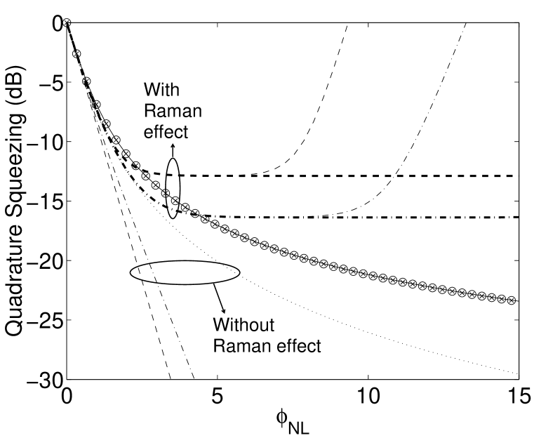
Fig. 5: Squeezing vs. nonlinear phase shift in a lossless fiber. Lower lines, without Raman effect. Upper lines, with Raman effect. Dashed lines signify that phase-matching is achieved at the input [$\Delta k=-2{\rm Re}\{\gamma_{\Omega}\}|A_{p}|^{2}$]. The thick dashed line is for optimal LO power splitting, thin dashed lines for equal LO power splitting. Dash-dotted lines are for $\Delta k=-(2/3){\rm Re}\{\gamma_{\Omega}\}|A_{p}|^{2}$. Thick dash-dotted line is for optimal LO power splitting, thin dashed lines for equal LO power splitting. In all other lines, $\Delta k=0$. Raman effect neglected, dotted line; Raman effect included and equal LO power splitting, marked with x; Raman effect included and optimal LO power splitting, circles; CW limit of Eq. (100) with $\bar{\gamma}_{i}^{{}^{\prime}}(0)kT/\hbar\bar{\gamma}_{0}=0.026$, thin solid line. Pump-signal detuning is 40 GHz.

References

• [1] K. K. Y. Wong, K. Shimizu, M. E. Marhic, K. Uesaka, G. Kalogerakis, and L. G. Kazovsky, “Continuous-wave fiber optical parametric wavelength converter with 40 dB conversion efficiency and a 3.8-dB noise figure,” Opt. Lett. 28, 692–694 (2003).
• [2] J. Hansryd, P. A. Andrekson, M. Westlund, J. Li, and P. Hedekvist, “Fiber-Based Optical Parametric Amplifiers and their Applications,” IEEE J. of Sel. Top. in Quantum Electron. 8, 506–520 (2002).
• [3] Y. Su, L. Wang, A. Agarwal, and P. Kumar, “Wavelength-Tunable All-Optical Clock Recovery Using a Fiber-Optic Parametric Oscillator,” Opt. Comm. 184, 151 (2000).
• [4] L. Wang, Y. Su, A. Agarwal, and P. Kumar, “Synchronously Mode-Locked Fiber Laser Based on Parametric Gain Modulation and Soliton Shaping,” Opt. Commun. 194, 313–317 (2001).
• [5] L. Wang, A. Agarwal, Y. Su, and P. Kumar, “All-Optical Picosecond-Pulse Packet Buffer Based on Four-Wave Mixing Loading and Intracavity Soliton Control,” IEEE J. of Quantum Electron. 38, 614–619 (2002).
• [6] J. L. Blows and S. E. French, “Low-noise-figure optical parametric amplifier with a continuous-wave frequency-modulated pump,” Opt. Lett. 27, 491–493 (2002).
• [7] R. Tang, J. Lasri, P. Devgan, J. E. Sharping, and P. Kumar, “Record performance of parametric amplifier constructed with highly nonlinear fibre,” Electron. Lett. 39 (2003).
• [8] S. Radic, C. J. McKinstrie, R. M. Jopson, J. Centanni, Q. Lin, and G. Agrawal, “Record performance of parametric amplifier constructed with highly nonlinear fibre,” Electron. Lett. 39 (2003).
• [9] P. L. Voss, R. Y. Tang, and P. Kumar, “Measurement of the photon statistics and the noise figure of a fiber-optic parametric amplifier,” Opt. Lett. 28, 549–551 (2003).
• [10] P. L. Voss and P. Kumar, “Raman-noise induced noise-figure limit for $\chi^{(3)}$ parametric amplifiers,” Opt. Lett. 29, 445–447 (2004).
• [11] P. Voss and P. Kumar, “Raman-effect induced noise limits on $\chi^{(3)}$ parametric amplifiers and wavelength converters,” J. Optic. B. 6, S762–S770 (2004).
• [12] R. Tang, P. L. Voss, J. Lasri, P. Devgan, and P. Kumar, “Noise-figure of a fiber parametric amplifier and wavelength converter: Experimental investigation,” Opt. Lett. 29, 2372–2374 (2004).
• [13] M. E. Marhic, C. H. Hsia, and J. M. Jeong, “Optical amplification in a nonlinear fiber interferometer,” Electron. Lett. 27, 201 (1991).
• [14] G. Bartolini, R. D. Li, P. Kumar, W. Riha, and K. V. Reddy, “1.5-mm phase-sensitive amplifier for ultrahigh-speed communications,” in Proc. OFC’94, pp. 202–203 (1994).
• [15] C. M. Caves, “Quantum Limits on Noise in Limited Amplifiers,” Phys. Rev. D 26, 1817–1839 (1982).
• [16] W. Imajuku, A. Takada, and Y. Yamabayashi, “Inline coherent optical amplifier with noise figure lower than 3dB quantum limit,” Electron. Lett. 36 (2000).
• [17] D. Levandovsky, M. Vasilyev, and P. Kumar, “Near-noiseless amplification of light by a phase-sensitive fibre amplifier,” Pramana J. Phys. 2–3 (2001).
• [18] R. M. Shelby, M. D. Levenson, and P. W. Bayer, “Guided acoustic-wave Brillouin scattering,” Phys. Rev. B 31, 5244– 5252.
• [19] K. Bergman, H. A. Haus, E. P. Ippen, and M. Shirasaki, “Squeezing in a Fiber Interferometer with a Gigahertz Pump,” Opt. Lett. 19, 290–292 (1994).
• [20] R. Tang, P. Devgan, P. L. Voss, V. Grigoryan, and P. Kumar, “An in-line frequency-nondegenerate phase-sensitive fiber-optical parametric amplifier,” Photon. Tech. Lett. 17, 1845 (2005).
• [21] R. Tang, P. Devgan, V. Grigoryan, and P. Kumar, “In-line frequency-non-degenerate phase-sensitive fiber parametric amplifier for fiber-optic communications,” Accepted for publication in Electron. Lett. (2005).
• [22] M. Vasilyev, “Distributed Phase Sensitive Amplification,” Submitted to Optics Express (2005).
• [23] H. P. Yuen, “2-Photon Coherent States Of Radiation-Field,” Phys. Rev. A 13, 2226–2243 (1976).
• [24] H. P. Yuen and J. H. Shapiro, “Optical Communication With 2-Photon Coherent States .1. Quantum-State Propagation And Quantum-Noise Reduction,” IEEE Trans. Inf. Theory 24, 657–668 (1978).
• [25] J. H. Shapiro, H. P. Yuen, and J. A. M. Mata, “Optical Communication with 2-Photon Coherent States .2. Photoemissive Detection and Structured Receiver Performance,” IEEE Trans. Inf. Theory 25, 179–192 (1979).
• [26] H. P. Yuen and J. H. Shapiro, “Optical Communication with 2-Photon Coherent States .3. Quantum Measurements Realizable with Photo-Emissive Detectors,” IEEE Trans. Inf. Theory 26, 78–82 (1980).
• [27] C. M. Caves, “Quantum-mechanical noise in an interferometer,” Phys. Rev. D 23, 1693–1708 (1981).
• [28] N. Treps, N. Grosse, W. P. Bowen, C. Fabre, H. A. Bachor, and P. K. Lam, “A Quantum Laser Pointer,” Science 301, 940–943 (2003).
• [29] A. N. Boto, P. Kok, D. S. Abrams, S. L. Braunstein, C. P. Williams, and J. P. Dowling, “Quantum Interferometric Optical Lithography: Exploiting Entanglement to Beat the Diffraction Limit,” Phys. Rev. Lett. 86, 2736–2739 (2000).
• [30] J. H. Shapiro and L. Boivin, “Raman-Noise Limit on Squeezing in Continuous-Wave Four-Wave Mixing,” Opt. Lett. 20, 925–927 (1995).
• [31] L. Boivin, F. X. Kärtner, and H. A. Haus, “Analytical Solution to the Quantum Field Theory of Self-Phase Modulation with a Finite Response Time,” Phys. Rev. Lett. 73, 240–243 (1994).
• [32] F. X. Kärtner, D. J. Dougherty, H. A. Haus, and E. P. Ippen, “Raman noise and soliton squeezing,” J. Opt. Soc. B 11, 1267–1276 (1994).
• [33] P. D. Drummond and J. F. Corney, “Quantum Noise in Optical Fibers: I. Stochastic Equations,” J. of Opt. Soc. Amer. B 18, 139–152 (2001).
• [34] N. R. Newbury, “Raman gain: pump-wavelength dependence in single-mode fiber,” Opt. Lett. 27, 1232–1234 (2002).
• [35] N. R. Newbury, “Pump-wavelength dependence of Raman gain in single-mode optical fibers,” J. Lightwave Technol. 21, 3364–3373 (2003).
• [36] G. P. Agrawal, Nonlinear Fiber Optics, Third Edition (Academic Press, San Diego, CA, 2001).
• [37] E. Golovchenko, P. V. Mamyshev, A. N. Pilipetskii, and E. M. Dianov, “Mutual influence of the parametric effects and stimulated Raman scattering in optical fibers,” IEEE Journal of Quantum Electronics 26, 1815–1820 (1990).
• [38] S. J. Carter, P. D. Drummond, M. D. Reid, and R. M. Shelby, “Squeezing of quantum solitons,” Phys. Rev. Lett 58 (1987).
Refer to caption