Towards feedback control of entanglement

Abstract

We provide a model to investigate feedback control of entanglement. It consists of two distant (two-level) atoms which interact through a radiation field and becomes entangled. We then show the possibility to stabilize such entanglement against atomic decay by means of a feedback action.

1 Introduction

Over the last decade, the rapid development of quantum technology has led to the possibility of continuously monitoring an individual quantum system with very low noise and manipulating it on its typical evolution time scale mab99 . It is therefore natural to consider the possibility of controlling individual quantum systems in real time by using feedback. A theory of quantum-limited feedback has been introduced by Wiseman and Milburn wismil93 ; wis94 . Among recent developments we mention the feedback stabilization of the state of a two level atom (single qubit) against amplitude damping wanwis01 .

Because of the relevant role played by entanglement in quantum processes, it would be straightforward to also consider its feedback control. Here we extend the basic idea of Ref.wanwis01 to a recently proposed model manbos01 consisting of two distant (two-level) atoms (two qubit) which interact through a radiation field and becomes entangled. We then show the possibility to stabilize such entanglement against atomic decay by means of a feedback action.

2 The Model

We consider a very simple model consisting of two two-level atoms, $1$ and $2$, placed in distant cavities and interacting through a radiation field in a dispersive way. The two cavities are arranged in a cascade-like configuration such that, given a coherent input field with amplitude $A$ in one of them, the output of each cavity enters the other as depicted in Fig.1.

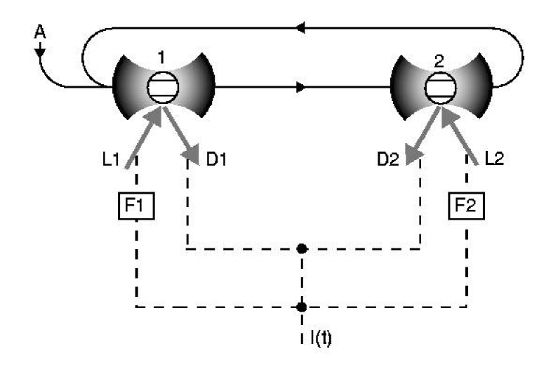
Figure 1: Schematic description of the considered set-up. Two distinct cavites, each containing a two-level atom ($1$ and $2$ respectively), are connected via radiation fields (solid lines). A coherent input of amplitude $A$ is provided in one of them. Furthermore, $L1$, $L2$ and $D1$, $D2$ represent local operations, namely driving fields and homodyne detection respectively. $I$ is the current arising from local measurements and $F1$, $F2$ indicate the consequent local feedback actions (dashed lines).

Then, it is possible to show manbos01 , after eliminating the radiation fields, that the effective interaction Hamiltonian for the internal degrees of the two atoms becomes of Ising type, namely

$$H_{int}=2J\sigma_{1}^{(z)}\sigma_{2}^{(z)}\,,$$ (1)

where $\sigma_{1,2}^{(x,y,z)}$ indicate the usual Pauli operators. Hereafter we shall also use $\sigma_{1,2}\equiv(\sigma_{1,2}^{(x)}+i\sigma_{1,2}^{(y)})/2$. The spin-spin coupling constant $J$ scales as radiation pressure $|A|^{2}$ and goes to zero for negligible cavity detuning manbos01 .

To get entanglement in an Ising model, it is necessary to break its symmetry gunetal01 . To this end, we consider local laser fields applied to each atom (L1 and L2 of Fig.1) such that a local Hamiltonian $H_{drive}$ given by

$$H_{drive}=\alpha\sigma_{1}^{(y)}+\alpha\sigma_{2}^{(y)},\qquad(\alpha\in{\bf R})$$ (2)

acts in addition to $H_{int}$. Thus, the total Hamiltonian of the system results

$$H_{tot}=H_{drive}+H_{int}.$$ (3)

Let us introduce the ground and excite atomic states $|g\rangle_{1,2}$, $|e\rangle_{1,2}$ as eigenvectors of $\sigma_{1,2}^{(z)}$ with $-1$ and $+1$ eigenvalues respectively, and $\eta\equiv\alpha/J$. Then, the eigenvectors of the Hamiltonian $H_{tot}$ read

$$|\psi_{1}\rangle = \frac{\eta}{2\sqrt{1+\eta^{2}+\sqrt{1+\eta^{2}}}}\left(|g\rangle_{1}|g\rangle_{2}-|e\rangle_{1}|e\rangle_{2}\right)$$

$$+i\frac{1+\sqrt{1+\eta^{2}}}{2\sqrt{1+\eta^{2}+\sqrt{1+\eta^{2}}}}\left(|e\rangle_{1}|g\rangle_{2}+|g\rangle_{1}|e\rangle_{2}\right)\,,$$

$$|\psi_{2}\rangle = \frac{1}{\sqrt{2}}\left(|e\rangle_{1}|g\rangle_{2}-|g\rangle_{1}|e\rangle_{2}\right)\,,$$

$$|\psi_{3}\rangle = \frac{1}{\sqrt{2}}\left(|g\rangle_{1}|g\rangle_{2}+|e\rangle_{1}|e\rangle_{2}\right)\,,$$

$$|\psi_{4}\rangle = \frac{\eta}{2\sqrt{1+\eta^{2}-\sqrt{1+\eta^{2}}}}\left(|g\rangle_{1}|g\rangle_{2}-|e\rangle_{1}|e\rangle_{2}\right)$$

$$+i\frac{1-\sqrt{1+\eta^{2}}}{2\sqrt{1+\eta^{2}-\sqrt{1+\eta^{2}}}}\left(|e\rangle_{1}|g\rangle_{2}+|g\rangle_{1}|e\rangle_{2}\right)\,,$$

with eigenvalues $E_{1}=-2\sqrt{\alpha^{2}+J^{2}}$, $E_{2}=-2J$, $E_{3}=2J$ and $E_{4}=2\sqrt{\alpha^{2}+J^{2}}$.

It is reasonable to consider as initial state of the two atoms the ground state $|g\rangle_{1}|g\rangle_{2}$; then we can expand it over the eigenstates basis (2) as

$$|\Psi(0)\rangle\equiv|g\rangle_{1}|g\rangle_{2}=\sum_{j=1}^{4}C_{j}|\psi_{j}\rangle\,,$$ (5)

with

$$C_{1} = -\frac{\left(1-\sqrt{1+\eta^{2}}\right)\sqrt{1+\eta^{2}+\sqrt{1+\eta^{2}}}}{2\eta\sqrt{1+\eta^{2}}}\,,$$

$$C_{2} = 0\,,$$

$$C_{3} = \frac{1}{\sqrt{2}}\,,$$

$$C_{4} = \frac{\left(1+\sqrt{1+\eta^{2}}\right)\sqrt{1+\eta^{2}-\sqrt{1+\eta^{2}}}}{2\eta\sqrt{1+\eta^{2}}}\,.$$ (6)

3 System dynamics

The evolution of the state (5) under $H_{tot}$ gives

$$|\Psi(t)\rangle = C_{1}e^{2i\tau\sqrt{1+\eta^{2}}}|\psi_{1}\rangle$$ (7)

$$+C_{2}e^{-2i\tau}|\psi_{2}\rangle$$

$$+C_{4}e^{-2i\tau\sqrt{1+\eta^{2}}}|\psi_{4}\rangle\,,$$

where we have introduced the scaled time $\tau=Jt$.

In Ref.wanwis01 it was shown that homodyne measurement of the light scattered by an atom allows indirect measurement of its spin flip operators. Then, let us consider, such type of local measurements so that after combining homodyne currents, the total current $I(t)$ carries out information about the observable ${\cal O}\equiv\sigma_{1}^{(x)}-\sigma_{2}^{(x)}$. Its variance over the state (7) is

$$\langle\Psi(t)|{\cal O}^{2}|\Psi(t)\rangle-\langle\Psi(t)|{\cal O}|\Psi(t)\rangle^{2}$$

$$=2-\frac{\eta^{2}}{1+\eta^{2}}\left[1-\cos\left(4\tau\sqrt{1+\eta^{2}}\right)\right]\,.$$ (8)

Notice that this quantity being strictly less than $2$ at almost any time, shows the presence of correlations for the state (7). On the other hand, in Ref.manbos01 it has been shown that the state (7) exhibits entanglement at almost any time. We are thus led to ascribe the correlations of Eq.(3) to the presence of entanglement in Eq.(7), though this would not generally true. Then, we are going to consider the quantity ${\cal O}$ as a “marker” of entanglement while characterizing the open system dynamics.

When we include the effect of spontaneous atomic decay at rate $\gamma$, the dynamics of the two distant atoms is described by the master equation

$$\dot{\rho} = -i\left[H_{tot},\rho\right]+{\bf D}\left[\sigma_{1}\right]\rho+{\bf D}\left[\sigma_{2}\right]\rho$$ (9)

$$\equiv -i\left[H_{tot},\rho\right]+{\bf D}\left[c_{+}\right]\rho+{\bf D}\left[c_{-}\right]\rho\,,$$

where $c_{\pm}=(\sigma_{1}\pm\sigma_{2})/\sqrt{2}$ and ${\bf D}$ is the Lindblad decoherence superoperator, i.e. ${\bf D}[a]b\equiv aba^{{\dagger}}-a^{{\dagger}}ab/2-ba^{{\dagger}}a/2$. The following replacements $J/\gamma\to J$, $\alpha/\gamma\to\alpha$, $\gamma t\to t$ have been made deriving Eq.(9).

The steady state solution of Eq.(9) can be easily found by writing the density operator in a matrix form, in the basis $\{|e\rangle_{1}|e\rangle_{2},|g\rangle_{1}|e\rangle_{2},|e\rangle_{1}|g\rangle_{2},|g\rangle_{1}|g\rangle_{2}\}$, as

$$\rho_{ss}=\left(\begin{array}[]{cccc}{\cal A}&{\cal B}_{1}+i{\cal B}_{2}&{\cal C}_{1}+i{\cal C}_{2}&{\cal D}_{1}+i{\cal D}_{2}\\ {\cal B}_{1}-i{\cal B}_{2}&{\cal E}&{\cal F}_{1}+i{\cal F}_{2}&{\cal G}_{1}+i{\cal G}_{2}\\ {\cal C}_{1}-i{\cal C}_{2}&{\cal F}_{1}-i{\cal F}_{2}&{\cal H}&{\cal I}_{1}+i{\cal I}_{2}\\ {\cal D}_{1}-i{\cal D}_{2}&{\cal G}_{1}-i{\cal D}_{2}&{\cal I}_{1}-i{\cal I}_{2}&{\cal L}\end{array}\right)\,,$$ (10)

while the matrix representation of the other operators (in the same basis) comes from

$$\sigma_{1}=\left(\begin{array}[]{cccc}0&0&0&0\\ 1&0&0&0\\ 0&0&0&0\\ 0&0&1&0\end{array}\right)\,,\quad\sigma_{2}=\left(\begin{array}[]{cccc}0&0&0&0\\ 0&0&0&0\\ 1&0&0&0\\ 0&1&0&0\end{array}\right)\,.$$ (11)

By inserting these matrices in the r.h.s. of Eq.(9) and equating to $0$ at l.h.s. we are left with a set of $16$ linear equations from which we can calculate (together with the normalization condition ${\rm tr}(\rho)=1$) all the real coefficients of the matrix (10), namely

$${\cal A} = \frac{1}{\Xi}16\alpha^{4},$$

$${\cal B}_{1} = -\frac{1}{\Xi}8\alpha^{3},\qquad{\cal B}_{2}=0,$$

$${\cal C}_{1} = -\frac{1}{\Xi}8\alpha^{3},\qquad{\cal C}_{2}=0,$$

$${\cal D}_{1} = \frac{1}{\Xi}4\alpha^{2},\qquad{\cal D}_{2}=\frac{1}{\Xi}16\alpha^{2}J,$$

$${\cal E} = \frac{1}{\Xi}\left(16\alpha^{4}+4\alpha^{2}\right),$$

$${\cal F}_{1} = \frac{1}{\Xi}4\alpha^{2},\qquad{\cal F}_{2}=0,$$

$${\cal G}_{1} = -\frac{1}{\Xi}2\alpha(4\alpha^{2}+1),\qquad{\cal G}_{2}=-\frac{1}{\Xi}8\alpha J,$$

$${\cal H} = \frac{1}{\Xi}\left(16\alpha^{4}+4\alpha^{2}\right),$$

$${\cal I}_{1} = -\frac{1}{\Xi}2\alpha(4\alpha^{2}+1),\qquad{\cal I}_{2}=-\frac{1}{\Xi}8\alpha J,$$

$${\cal L} = \frac{1}{\Xi}\left(16\alpha^{4}+8\alpha^{2}+1+16J^{2}\right),$$ (12)

with

$$\Xi=64\alpha^{4}+16\alpha^{2}+1+16J^{2}\,.$$ (13)

4 Stationary entanglement

One can use the concurrence as measure of the degree of entanglement between two qubit described by density operator $\rho$ woo98 . It is defined as

$$C(\rho)=\max\left\{0,\xi_{1}-\xi_{2}-\xi_{3}-\xi_{4}\right\}$$ (14)

where $\xi_{i}$’s are, in decreasing order, the nonnegative square roots of the moduli of the eigenvalues of the non-hermitian matrix $\rho\tilde{\rho}$. Here $\tilde{\rho}$ is the matrix given by

$$\tilde{\rho}\equiv\left(\sigma_{1}^{(y)}\otimes\sigma_{2}^{(y)}\right)\rho^{*}\left(\sigma_{1}^{(y)}\otimes\sigma_{2}^{(y)}\right)\,,$$ (15)

where $\rho^{*}$ denotes the complex conjugate.

The stationary state concurrence $C_{0}\equiv C(\rho_{ss})$ is shown in Fig.2.

Figure 2: Concurrence $C_{0}$ of the steady state plotted versus the driving strength $\alpha$ and the coupling constant $J$.

It is clear that a relevant amount of entanglement persists at steady state only for large values of the coupling constant, i.e. $J\gg 1$, (when the original $J$ is much greater than $\gamma$).

5 Feedback action

We can now think to stabilize the entanglement, i.e. to prevent its degradation, by using a feedback action on the driving fields (L1 and L2 of Fig.1) accordingly to the measured quantity ${\cal O}$ which should reveal the status of nonclassical correlations. Then we act on the system with a local feedback operator

$$F\equiv\frac{\lambda}{\sqrt{2}}\left(\sigma_{1}^{(y)}-\sigma_{2}^{(y)}\right)\,,$$ (16)

where $\lambda$ represent the feedback strength (already scaled by $\gamma$, i.e. $\lambda/\sqrt{\gamma}\to\lambda$). The choice of $F$ is motivated by the fact that feedback mediated by indirect (homodyne) measurement requires, to squeeze the variance of a variable (${\cal O}$), a driving action on the conjugate variable man00 .

The master equation (9) then becomes wis94

$$\dot{\rho} = -i\left[H_{tot},\rho\right]+{\bf D}\left[c_{+}\right]\rho$$ (17)

$$+{\bf D}\left[c_{-}-iF\right]\rho-\frac{i}{2}\left[c_{-}^{{\dagger}}F+Fc_{-},\rho\right]\,.$$

In the above equation, the feedback operator $F$ appears in the Hamiltonian term describing the driving effect, as well as inside the decoherence superoperator accounting for quantum noise carried back into the system from measurement.

The master equation (17) can be solved at steady state with the same method of Eq.(9), obtaining $\rho^{fb}_{ss}$. However, the analytical expression is quite cumbersome, hence not reported at all. The state $\rho^{fb}_{ss}$ allows us to (numerically) calculate its concurrence. In particular, we have evaluate the quantity

$$C_{fb}\equiv\max_{\lambda\in{\bf R}}C(\rho^{fb}_{ss})\,,$$ (18)

that is shown in Fig.3.

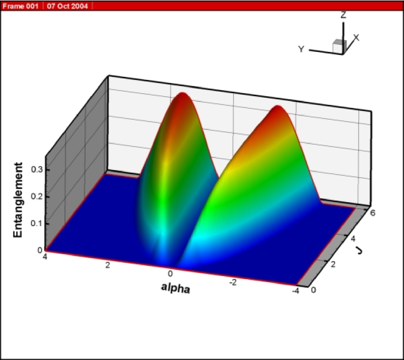
Figure 3: Concurrence $C_{fb}$ of the steady state plotted versus the driving strength $\alpha$ and the coupling constant $J$ in presence of feedback action. For each value of $\alpha$ and $J$, the feedback strength is chosen to be the optimal.

We can see that feedback improves the available entanglement with respect to previous case (Fig.2). Feedback seems especially powerful at small values of $J$ where entanglement was very fragile (it somehow enforces the coupling effect).

To better compare the results with and without feedback, in Fig.4 we have shown the difference $C_{fb}-C_{0}$.

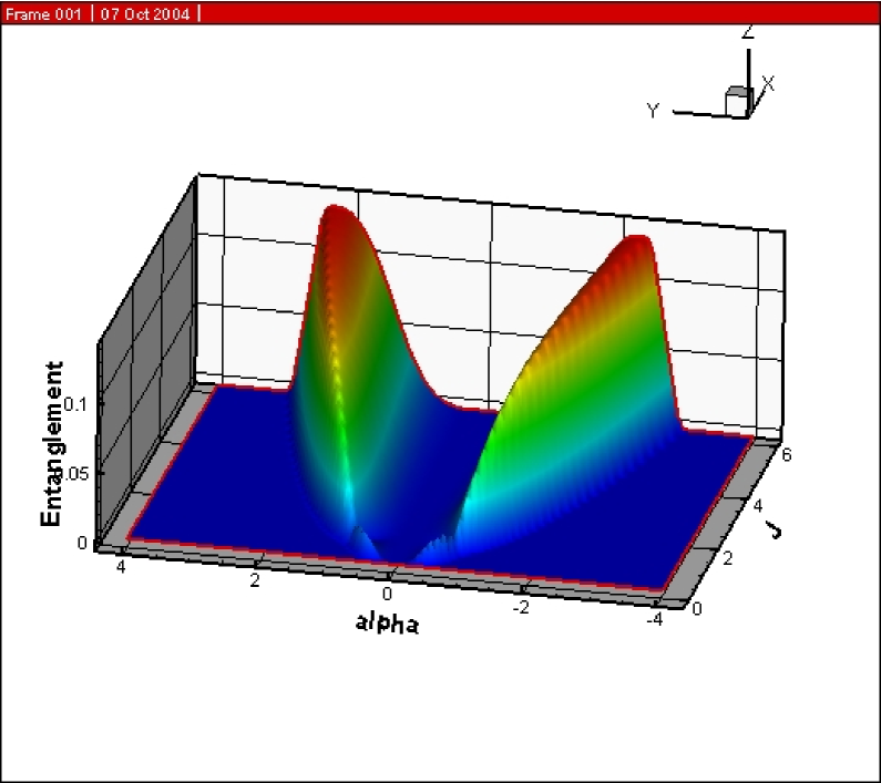
Figure 4: Concurrences difference $C_{fb}-C_{0}$ plotted versus the driving strength $\alpha$ and the coupling constant $J$.

6 Conclusion

We have shown the possibility to improve the steady state entanglement in an open quantum system by using a feedback action. Although the improvement is not very high the above result represents a proof of principle about the possibility of controlling entanglement through feedback. A complementary possibility to increase entanglement between atoms subject to joint measurements with feedback has been then proposed wanwismil04 .

Since our method only relies on Local Operations and Classical Communication (LOCC), what we have obtained is perhaps related to entanglement purification ben96 .

To improve the presented model one should find the best entanglement witness ecketal03 to measure, and then optimize the feedback action (operator). This can be phrased in terms of a numerical optimization problem and is left for future work. Moreover, since entanglement is a system state peculiarity, other feedback procedures, like state estimation based feedback doh99 , could be more powerful.

Summarizing, although we have proved the possibility of feedback control of entanglement, its effectiveness remains difficult to quantify in nonlinear systems (like that studied). Probably, investigations in linear systems would be more fruitful.

References

- (1) H. Mabuchi, J. Ye and H. J. Kimble, Appl. Phys. B 68, (1999) 1095; W. P. Smith, J. E. Reiner, L. A. Orozco, S. Kuhr and H. M. Wiseman, Phys. Rev. Lett. 89, 133601 (2002); J. M. Geremia, J. K. Stockton and H. Mabuchi, Science 304, (2004) 270.
- (2) H. M. Wiseman and G. J. Milburn, Phys. Rev. Lett. 70, (1993) 548.
- (3) H. M. Wiseman, Phys. Rev. A 49, (1994) 2133.
- (4) J. Wang and H. M. Wiseman, Phys. Rev. A 64, (2001) 063810; H. M. Wiseman, S. Mancini and J. Wang, Phys. Rev. A 66, (2002) 013807.
- (5) S. Mancini and S. Bose, Phys. Rev. A 70, 022307 (2004).
- (6) D. Gunlycke, S. Bose, V. M. Kendon and V. Vedral, Phys. Rev. A 64, (2001) 042302.
- (7) H. M. Wiseman and G. J. Milburn, Phys. Rev. A 49, (1994) 1350.
- (8) W. K. Wootters, Phys. Rev. Lett 80, 2245 (1998).
- (9) S. Mancini, D. Vitali and P. Tombesi, Phys. Rev. A 61, (2000) 053404.
- (10) J. Wang, H. M. Wiseman and G. J. Milburn, arXiv:quant-ph/0409154.
- (11) C. H. Bennett, G. Brassard, S. Popescu, B. Schumacher, J. A. Smolin and W. K. Wootters, Phys. Rev. Lett. 76, (1996) 722.
- (12) D. Bruss, J. Math. Phys. 43, 4237 (2002).
- (13) A. C. Doherty and K. Jacobs, Phys. Rev. A 60, (1999) 2700.