Cloning transformations in spin networks without external control

Abstract

In this paper we present an approach to quantum cloning with unmodulated spin networks. The cloner is realized by a proper design of the network and a choice of the coupling between the qubits. We show that in the case of phase covariant cloner the $XY$ coupling gives the best results. In the $1\to 2$ cloning we find that the value for the fidelity of the optimal cloner is achieved, and values comparable to the optimal ones in the general $N\to M$ case can be attained. If a suitable set of network symmetries are satisfied, the output fidelity of the clones does not depend on the specific choice of the graph. We show that spin network cloning is robust against the presence of static imperfections. Moreover, in the presence of noise, it outperforms the conventional approach. In this case the fidelity exceeds the corresponding value obtained by quantum gates even for a very small amount of noise. Furthermore we show how to use this method to clone qutrits and qudits. By means of the Heisenberg coupling it is also possible to implement the universal cloner although in this case the fidelity is $10\%$ off that of the optimal cloner.

I Introduction

The no-cloning theorem WZ82 states that it is impossible to make perfect copies of an unknown quantum state. At variance with the classical world, where it is possible to duplicate information faithfully, the unitarity of time evolution in quantum mechanics does not allow us to build a perfect quantum copying machine. This no-go theorem is at the root of the security of quantum cryptography gisin02 , since an eavesdropper is unable to copy the information transmitted through a quantum channel without disturbing the communication itself. Although perfect cloning is not allowed, it is, nevertheless, possible to produce several approximate copies of a given state. Several works, starting from the seminal paper by Bužek and M. Hillery BH96 , have been devoted to find the upper bounds to the fidelity of approximate cloning transformations compatible with the rules of quantum mechanics. Besides the theoretical interest on its own, applications of quantum cloning can be found in quantum cryptography, because they allow us to derive bounds for the security in quantum communication gisin02 , in quantum computation, where quantum cloning can be used to improve the performance of some computational tasks galvao , and in the problem of state estimation lopresti .

As mentioned above, the efficiency of the cloning transformations is usually quantified in terms of the fidelity of each output cloned state with respect to the input. The largest possible fidelity depends on several parameters and on the characteristics of the input states. For an $N\to M$ cloner it depends on the number $N$ of the input states and on the number $M$ of output copies. It also depends on the dimension of the quantum systems to be copied. Moreover, the fidelity increases if some prior knowledge of the input states is assumed. In the universal cloning machine the input state is unknown. A better fidelity is achieved, for example, in the phase covariant cloner (PCC) where the state is known to lie on the equator of the Bloch sphere (in the case of qubits). Upper bounds to the fidelity for copying a quantum state were obtained in Refs. BH96 and  bruss98 in the case of universal and state dependent cloning respectively. The more general problem of copying $N\to M$ qubits has been also addressed cloner_n-m . The PCC has been proposed in Ref. bruss00 . Several protocols for implementing cloning machines have been already achieved experimentally cummins02 ; bouwmeester02 ; demartini ; ekert03 . In all the above proposals the cloning device is described in terms of quantum gates, or otherwise is based on post-selection methods. For example, the quantum network corresponding to the $1\to 2$ PCC consists of two controlled-not (C-NOT) gates together with a controlled rotation niu99 .

The implementation of given tasks by means of quantum gates is not the the only way to execute the required quantum protocols. Recently it has been realized that there are situations where it is sufficient to find a proper architecture for the qubit network and an appropriate form for the coupling between qubits to achieve the desired task. Under these conditions the execution of a quantum protocol is reached by the time evolution of the quantum-mechanical system. The only required control is on the preparation of the initial state of the network and on the read-out after the evolution. This perspective is certainly less flexible than the traditional approach with quantum gates. Nevertheless it offers great advantages as it does not require any time modulation for the qubits couplings. Moreover, among the reasons for this “no-control” approach to quantum information is that the system is better isolated from the environment during its evolution. This is because there is no active control on the Hamiltonian of the system. Actually, after initializing the network one needs only to wait for some time (to be determined by the particular task) and then read the output. Several examples have been provided so far. A spin network for quantum computation based only on Heisenberg interactions has been proposed benjamin03 ; yung . Another area where this approach is attracting increasing attention is quantum communication, where spin chains have been proposed as natural candidates of quantum channels bose ; subra03 ; datta ; osborne ; lloyd ; cirac ; giovannetti . An unknown quantum state can be prepared at one end of the chain and then transferred to the other end by simply employing the ability of the chain to propagate the state by means of its dynamical evolution. These proposals seem to be particularly suited for solid state quantum information, where schemes for implementation have already been put forward romito ; paternostro .

Stimulated by the above results in quantum communication we have studied quantum cloning in this framework. The main goal is to find a spin network and an interaction Hamiltonian such that at the end of its evolution the initial state of a spin is (imperfectly) copied on the state of a suitable set of the remaining spins. In this paper we will show that this is indeed possible and we will analyze various types of quantum cloners based on the procedure just described. We will describe a setup for the $N\to M$ PCC and we will show that for $N=1$ and $M=2$ the spin network cloning (SNC) achieves the optimal bound. We will also describe the more general situation of cloning of qudits, i.e. d-level systems. An important test is to compare the performance of our SNC with the traditional approach using quantum gates. We show that in the (unavoidable) presence of noise our method is far more robust. Some of the results have been already given in Ref. dechiara . In the present paper we will give many additional details, not contained in Ref. dechiara , and extend our approach to cloning to several other situations. We discuss cloning of qutrits, universal cloning machines, and optimization of the model Hamiltonian just to mention few extentions.

The paper is organized as follows. In Section II we review the basic properties of approximate cloning showing the theoretical optimal bounds. In Section III we present the models and the networks topologies considered in this work. In Sections IV and V we briefly review and extend the results obtained in dechiara . These sections concern the spin network model to implement the $1\to M$ and $N\to M$ phase covariant cloning transformations respectively. In addition to a more detailed discussion, as compared to dechiara , here we present a detailed analysis of the role of static imperfections. We also optimize the cloning protocol over the space of a large class of model Hamiltonians which includes the $XY$ and Heisenberg as limiting cases.

The effects of noise, included in a fully quantum mechanical approach, are analyzed in Section VI, where we compare our cloning setup with cloning machines based on a gate design. In Sect. VII we study the possibility of achieving universal cloning with the spin network approach. In Section VIII we generalize the SNC for qutrits and qudits. Finally, in Section IX we propose a simple Josephson junctions circuit that realizes the protocol and in X we summarize the main results and present our conclusions.

II Optimal fidelities for Quantum Cloning

Most of this paper deals with the case of PCC. We will therefore devote this section to a brief summary of the results known so far for the optimal fidelity achievable in this case.

We start our discussion by considering quantum cloning of qubits, whose Hilbert space is spanned by the basis states $|0\rangle$ and $|1\rangle$. The most general state of a qubit can be parametrized by the angles $(\vartheta,\varphi)$ on the Bloch sphere as follows

$$|\psi\rangle=\cos\frac{\vartheta}{2}|0\rangle+e^{i\varphi}\sin\frac{\vartheta}{2}|1\rangle\,.$$ (1)

Quantum cloning was first analyzed BH96 , where the $1\to 2$ universal quantum cloning machine (UQCM) was introduced. We remind that the fidelity of a UQCM does not depend on $(\vartheta,\varphi)$ i.e. it is the same for all possible input states. As already mentioned, the quality of the cloner is quantified by means of the fidelity $\mathcal{F}$ of each output copy, described by the density operator $\rho$, with respect to the original state $|\psi\rangle$

$$\mathcal{F}=\langle\psi|\rho|\psi\rangle\;.$$ (2)

The value of the optimal fidelity is achieved by maximizing $\mathcal{F}$ over all possible cloning transformations. The result for the $1\to 2$ UQCM is $\mathcal{F}=5/6\simeq 0.83$ BH96 ; bruss98 . The general form of the optimal transformation, which requires an auxiliary qubit, has been explicitly obtained in Ref. bruss98 .

When the initial state is known to be in a given subset of the Bloch sphere, the value of the optimal fidelity generally increases. For example, in Ref. bruss98 cloning of just two non orthogonal states is studied and it is shown that the fidelity in this case is greater than that for the UQCM. The reason is that now some prior knowledge information on the input state is available. Another important class of transformations, which will be largely analyzed in the present paper, is the so called phase covariant cloning. In this type of cloner the fidelity is optimised equally well for all states belonging to the equator of the Bloch sphere:

$$|\psi\rangle=\frac{1}{\sqrt{2}}\left(|0\rangle+e^{i\varphi}|1\rangle\right)\;,$$ (3)

where $\varphi\in[0,2\pi]$. The optimal transformation for the $1\to 2$ PCC was found in bruss00 . The corresponding fidelity is given by

$$\mathcal{F}=\frac{1}{2}+\frac{1}{\sqrt{8}}\simeq 0.854\;.$$ (4)

In the $N\to M$ case of PCC, the optimal fidelities were derived in Ref. dariano03 . For the $1\to M$ PCC case they read footnote

$$\mathcal{F}= \frac{1}{2}\left(1+\frac{M+1}{2M}\right) \quad\textrm{for odd}\,M$$ (5)

$$\mathcal{F}= \frac{1}{2}\left(1+\frac{\sqrt{M(M+2)}}{2M}\right) \quad\textrm{for even}\,M$$ (6)

Optimal cloning has also been studied in higher dimensions. The universal case was discussed in Refs. werner98 . Cloning of qutrits was specifically treated in Refs. lopresti ; gisinqutrit , where the optimal fidelity for cloning some classes of states was derived. In particular the double-phase covariant symmetric $1\to 2$ cloner , which is optimized for input states of the form

$$|\psi\rangle=\frac{1}{\sqrt{3}}\left(|0\rangle+e^{i\varphi_{1}}|1\rangle+e^{i\varphi_{2}}|2\rangle\right)$$ (7)

where $\varphi_{1}$ and $\varphi_{2}$ are independent phases and the states $|0\rangle,|1\rangle,|2\rangle$ form a basis for a qutrit, was analyzed lopresti . The optimal $1\to M$ fidelity in the case of $M=3k+1$ (with $k$ positive integer) is given by the simple expression dariano03 :

$$\mathcal{F}=\frac{1}{3}\left(1+2\frac{M+2}{3M}\right)$$ (8)

For qudits, namely quantum systems with finite dimension $d$, the PCC is optimized for states of the form

$$|\psi\rangle=\frac{1}{\sqrt{d}}\sum_{i=0}^{d-1}e^{i\varphi_{i}}|i\rangle$$ (9)

where $\varphi_{0}=0$, while $\varphi_{1},\varphi_{2},\dots,\varphi_{d-1}$ are independent phases. The fidelity for $1\to 2$ PCC in dimension $d$ is given by matsu

$$\mathcal{F}=\frac{1}{d}+\frac{1}{4d}\left(d-2+\sqrt{d^{2}+4d-4}\right)\;.$$ (10)

More recently the general $N\to M$ case of PCC for qudits was analysed bdm , where explicit simple solutions were obtained for a number of output copies given by $M=kd+N$, with $k$ positive integer.

The quantum transformations corresponding to the cloning machines described above can be implemented by suitably designed quantum circuits. For example, in the $1\to 2$ and $1\to 3$ cases the circuits implementing PCC were derived in Refs. du and buzek97 respectively and they are shown in Fig.1 (note that in these cases no auxiliary qubits are needed).

a.
b.

Figure 1: a. Circuit implementing $1\to 2$ PCC for qubits and experimentally realized in du . b. Circuit implementing $1\to 3$ PCC buzek97 .

In Fig.1b. we defined $R_{i}=R_{y}(-2\vartheta_{i})$ and $\vartheta_{1}=\vartheta_{3}=\pi/8$ and $\vartheta_{2}=\arcsin\sqrt{\frac{1}{2}-\frac{\sqrt{2}}{3}}$.

This is not the only way to perform quantum cloning and quantum computation protocols in general. In the following sections we describe how to accomplish the desired task using the evolution of a spin network. The expressions for the fidelities given above will be compared to the ones derived by means of the approach proposed in Ref. dechiara and in the present paper.

III The spin network cloning

In this section we show how quantum cloning can be implemented using a spin network. First let us discuss our Hamiltonian model. We start with a fairly general model defined as

$$H_{\lambda}=\frac{1}{4}\sum_{ij}J_{ij}(\sigma^{i}_{x}\sigma^{j}_{x}+\sigma^{i}_{y}\sigma^{j}_{y}+\lambda\sigma^{i}_{z}\sigma^{j}_{z})+\frac{B}{2}\sum_{i}\sigma^{i}_{z}$$ (11)

where $\sigma^{i}_{x,y,z}$ are the Pauli matrices corresponding to the $i$-th site, $J_{ij}$ are the exchange couplings defined on the links joining the sites $i$ and $j$ and $B$ is an externally applied magnetic field. The anisotropy parameter $\lambda$ ranges from $0$ ($XY$ Model) to $1$ (Heisenberg Model). This model is named as the $XXZ$ Model. We discuss separately the two limiting cases $\lambda=1$ and $\lambda=0$. It turns out that for PCC the $\lambda=0$ case leads always to the highest fidelity. Given the model of Eq. (11) the fidelity is maximized over $B/J$ and $Jt$. We defined $B^{(M)}$ and $t^{(M)}$ the values of the parameters leading to the optimal solution. Notice that the total angular momentum as well as its $z$ component are always constants of motion independently of the topology of the network. In all the cases we consider in this work, the couplings $J_{ij}\neq 0$ only for nearest neighbors sites $i,j$. To specify which couplings are non-zero one has to define the topology of the spin network.

For the $1\to M$ PCC we choose $M+1$ spins in a star configuration (see fig. 2a). The central spin labeled by $1$ is initialized in the input state while the remaining M spins are the blank qubits and are initialized to the state $|0\rangle$ if $0<\vartheta<\pi/2$ and $|1\rangle$ if $\pi/2<\vartheta<\pi$. For this network $J_{ij}=J$ only if one of the two linked sites is the central one. This configuration has also been studied in a different context Bosestar . For the $1\to M$ case we have considered also other types of networks. These are represented in Fig.2b. The original state is placed on the top of the tree while the blank qubits are on the lowest level. The intermediary spins are ancillae. Each graph is characterized by the number $k$ of links departing from each site and the number $j$ of intermediate levels between the top and the blank qubits level. The number of blank qubits can be obtained from $j$ and $k$ as $M=k^{j+1}$. Notice that for this class of graphs a symmetry property holds: the global state of the blank qubits is invariant under any permutation of the $M$ qubits. For the $N\to M$ PCC we have considered a generalization of the star network (see Fig.2c). It consists of a star with N centers and M tips so no auxiliary qubits are present. Also this network is permutation invariant.

The cases defined above are not the most general networks and/or model Hamiltonian conceivable. Since the fidelity must be maximized over the parameters of the Hamiltonian as well as over the network topology one may wonder whether it is sufficient to consider only the cases introduced above. In Section IV.2 we partially answer to this question by considering the more general configuration for the $1\to 3$ case containing $4$ spins and we believe to have found the best possible scenario for the SNC. As far as the choice of the model Hamiltonian is concerned, the symmetry in the $XY$-plane is suggested by the phase covariance requirement for a PCC. We checked that the Ising model in transverse field, which is not phase covariant, gives poorer results for the fidelity. In principle one should also explore the possibility of multi-bit couplings, but we did not considered this (in principle interesting) situation. Multi-bit couplings are much more difficult to achieve experimentally and at the end of this work we want to propose to implement our scheme using Josephson nanocircuits, where two-qubit couplings with $XY$-symmetry are easy to realize.

Figure 2: Different topologies for $N\to M$ cloner: a) Spin star network for $1\to M$ cloner. b) Generic graph for the $1\to M$ cloner with $j$ intermediate steps and $k$ links departing from each vertex. c) Spin network for the $N\to M$ cloning

IV $1\to M$ PCC cloning

In this case the Hamiltonian (11) can be easily diagonalized because it can be mapped to the problem of a spin-1/2 interacting with a spin-M/2

$$H_{\lambda}=J\left(S^{1}_{x}S_{x}+S^{1}_{y}S_{y}+\lambda S^{1}_{z}S_{z}\right)+B(S^{1}_{z}+S_{z})\;\;.$$ (12)

where we have defined $S^{1}=\sigma^{1}/2$ and $S=1/2\sum_{2}^{M+1}\sigma^{i}$. The operators $S$ obey the usual commutation relations for an angular momentum operator. Notice that the modulus and the $z$ component of the total angular momentum $\vec{F}=\vec{S}^{1}+\vec{S}$ commute with the Hamiltonian. Thus the evolution is invariant under rotations around the $z$ axis. This property automatically makes our model a PCC.

For $0<\vartheta<\pi/2$ (the other case is equivalent) the initial state of the star is:

$$|\Psi(0)\rangle=\alpha|\underline{0}\rangle+\beta|\underline{1}\rangle$$ (13)

where $\alpha=\cos\frac{\vartheta}{2}$ and $\beta=e^{i\varphi}\sin\frac{\vartheta}{2}$. Here we use the convention that $|\underline{0}\rangle=|\underbrace{0\cdots 0}_{M+1}\rangle$ and $|\underline{j}\rangle=|\underbrace{0\cdots 1\cdots 0}_{M+1}\rangle$ where only the site $j$th is in the state $|1\rangle$.

Because of the conservation of the total angular momentum the state of the star at time $t$ will be a linear combination of $|\underline{0}\rangle$ and $|\underline{j}\rangle$ i.e. states with only one qubit in state $|1\rangle$. The state at time $t$ can thus be written in the form (apart from a global phase factor):

$$|\Psi(t)\rangle=\alpha|\underline{0}\rangle+\beta_{1}(t)|\underline{1}\rangle+\beta_{2}(t)\frac{1}{\sqrt{M}}\sum_{j=2}^{M+1}|\underline{j}\rangle$$ (14)

where the coefficients $\beta_{1}(t)$ and $\beta_{2}(t)$ depend on the particular choice of the Hamiltonian. In order to calculate the fidelity of the clones we need the expression for the reduced density matrix of one site. For symmetry reasons this is independent on the site chosen, the result being

$$\rho(t)=\left(\begin{array}[]{cc}|\alpha|^{2}+|\beta_{1}|^{2}+\left(1-\frac{1}{M}\right)|\beta_{2}|^{2}&\frac{\alpha\beta_{2}^{*}}{\sqrt{M}}\\ \frac{\alpha^{*}\beta_{2}}{\sqrt{M}}&\frac{|\beta_{2}|^{2}}{M}\end{array}\right)\;\;.$$ (15)

The fidelity for the SNC is

$$\mathcal{F}_{\lambda} = |\alpha|^{2}\left[|\alpha|^{2}+|\beta_{1}|^{2}+\left(1-\frac{1}{M}\right)|\beta_{2}|^{2}\right]$$ (16)

$$+ \frac{|\beta_{1}\beta_{2}|^{2}}{M}+2\textrm{Re}\left[\frac{|\alpha|^{2}\beta_{1}^{*}\beta_{2}}{\sqrt{M}}\right]$$

where the coefficients $\beta_{i}(t)$ depend explicitly on the chosen model (Heisenberg or $XY$ in this case).

Heisenberg model - Let us start with the Heisenberg model ($\lambda=1$) and let $B=0$ (we checked that a finite external magnetic field is not necessary to achieve the maximum fidelity). The Hamiltonian can be rewritten in the form $H=J\vec{S}^{1}\cdot\vec{S}$ and using $\vec{S^{1}}\cdot\vec{S}=1/2(F^{2}-S^{2}-S_{1}^{2})$ one finds that the eigenenergies are given by $E(F,S,S^{1})=\frac{J}{2}\left[F(F+1)-S(S+1)-S^{1}(S^{1}+1)\right]$ where $F,S,S^{1}$ are the quantum numbers associated to the corresponding operators. The eigenvectors can be found in terms of the Clebsch-Gordan coefficients. The results for the coefficients $\beta_{i}(t)$ are:

$$\beta_{1}(t) = \beta\frac{1}{1+2S}\left[2S\,e^{i\left(\frac{1}{2}+S\right)t}+1\right]$$ (17)

$$\beta_{2}(t) = \beta\frac{\sqrt{2S}}{1+2S}\left[1-e^{i\left(\frac{1}{2}+S\right)t}\right]$$ (18)

where $S=M/2$.

The maximum value for the fidelity

$$\mathcal{F}_{1}=\frac{4+M\,(3+M)+(M-1)[(3+M)\cos\vartheta-\cos 2\vartheta]}{2{(1+M)}^{2}}$$ (19)

is obtained for the parameters $Jt^{(M)}=2\pi/(M+1)$.

$XY$ model - Now let us turn our attention to the $XY$ model. Solving the eigenvalue problem as in Bosestar one finds

$$\beta_{1}(t) = \beta e^{iBt}\cos\frac{J}{2}\sqrt{M}t$$ (20)

$$\beta_{2}(t) = -i\beta e^{iBt}\sin\frac{J}{2}\sqrt{M}t$$ (21)

The fidelity is maximized when $B^{(M)}/J=\sqrt{M}/2$ and $Jt^{(M)}=\pi/\sqrt{M}$:

$$\mathcal{F}_{0}=\frac{(1+{\sqrt{M}})^{2}-\left(2-2M\right)\cos\vartheta+\left(1-{\sqrt{M}}\right)\cos 2\vartheta}{4M}$$ (23)

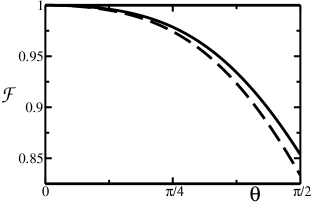
Figure 3: The fidelity $\mathcal{F}_{\lambda}$ for $M=2$ versus $\vartheta$ for the $XY$ (solid) and Heisenberg (dashed) model are shown. Notice that the optimal fidelity for the PCC is exactly that of the $XY$ model.

For $(\lambda=0)$ the fidelity is always greater than for $(\lambda=1)$. Let us analyze the previous results in two important cases. First let us discuss the case $M=2$ for arbitrary $\vartheta$ (see Fig.3):

$$\mathcal{F}_{1} = \frac{14+5\cos\vartheta-\cos 2\vartheta}{18}$$ (24)

$$\mathcal{F}_{0} = \frac{1}{8}(5+2\cos\vartheta+\cos 2\vartheta+2{\sqrt{2}}\sin^{2}\vartheta)$$ (25)

The fidelity $\mathcal{F}_{0}$ coincides with the fidelity for the $1\to 2$ PCC fiurasek03 i.e. the SNC saturates the optimal bound for the $1\to 2$ PCC. Second let us consider $\vartheta=\pi/2$ and arbitrary M (see Fig.4):

$$\mathcal{F}_{1} = \frac{1}{2}+\frac{1}{1+M}$$ (26)

$$\mathcal{F}_{0} = \frac{1}{2}\left(1+\frac{1}{\sqrt{M}}\right)$$ (27)

For $M>2$, $\mathcal{F}_{\lambda}$ is always smaller than the optimal fidelity given in Ref.dariano03 . Also in this case the XY model is better suited for quantum cloning as compared to the Heisenberg case. Although for generic $M$ the SNC does not saturate the optimal bound, there is a very appealing feature of this methods which makes it interesting also in this case. The time required to clone the state decreases with $M$. This implies that, in the presence of noise, SNC may be competitive with the quantum circuit approach, where the number of gates are expected to increase with $M$. We analyze this point in Section VI.

Recently a PCC with the star configuration has been proposed also for a multi-qubit cavity olayacastro . In this proposal the central spin is replaced by a bosonic mode of the cavity. By restricting the dynamics in the subspace with only one excitation (one excited qubit or one photon in the cavity) the Hamiltonian is equivalent to the $XY$ spin star network considered here. Indeed the optimal fidelities coincide with $\mathcal{F}_{0}$, Eq.(27).

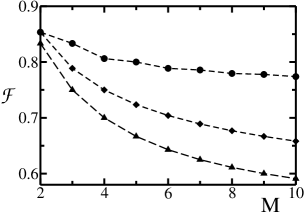
Figure 4: The fidelity $\mathcal{F}$ for PCC (circle), $XY$ (diamond) and Heisenberg (triangle) as functions of $M$ for $\vartheta=\pi/2$.

All the results discussed so far have been obtained for the star network. Obviously this is not the only choice which fulfills the symmetries of a quantum cloning network. In general one should also consider more general topologies and understand to what extent the fidelity depends on the topology. We analyzed this issue by studying the fidelity for the $XY$ model and $\vartheta=\pi/2$ for $M\leq 32$ for the graph b of Fig.2 (the fidelity for Heisenberg model in this case is much worse than in the star configuration). We conclude that the maximum fidelity obtained does not depend on the chosen graph.

IV.1 Imperfections

To assess the robustness of our protocol, it is important to analyze the effect of static imperfections in the network. In a nanofabricated network, as for example with Josephson nanocircuits, one may expect small variations in the qubit couplings. Here we analyze the $1\to M$ cloning assuming that the couplings $J_{ij}$ have a certain degree of randomness. For each configuration of disorder $J_{1i}$ are assigned in an interval of amplitude $2\epsilon$ centered around $J=1$ with a uniform distribution. First we study the case of uncorrelated disorder in different links. The values of $B$ and $t$ are chosen to be the optimal values of the ideal situation. For a given configuration of the couplings the fidelities of each of the clones are different due to the different coupling with the central spin. Only the average fidelity is again symmetric under permutation among the clones. We averaged the fidelity over the $M$ sites and over $10^{3}$ realization of disorder. For $\epsilon=10^{-1}$ and $M\leq 10$ the mean fidelity decreases by just less than $0.2\%$ of the optimal value. It is important to stress that the effect of imperfections is quite weak on the average fidelity. This is because for certain values of $J_{ij}$, even if the fidelity of a particular site can become much larger than the fidelity in the absence of disorder, at the same time for the same parameters the fidelity in other sites is very small and the average fidelity is weakly affected by imperfections. In figure 5 we show the fidelity for the $1\to 2$ SNC with imperfections as a function of the tolerance $\epsilon$. We study also the case with correlations between the signs of nearest neighbor bonds: the probability of equal signs $(J_{1i}-J)(J_{1i+1}-J)>0$ is proportional to $\mu\in[-1;1]$. The uncorrelated results are recovered for $\mu=0$. As expected this type of disorder is more destructive as shown in figure 5.

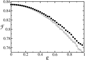
Figure 5: Mean fidelity for the $1\to 2$ case with static imperfections as a function of the tolerance $\epsilon$ with $\mu=0$ (filled squares) and $\mu=0.5$ (empty circles).

IV.2 Optimal network Hamiltonian for $1\to 3$ PCC

As shown in Fig.4, the $1\to 2$ SNC saturates the PCC optimal bound. However this is not the case for $M>2$, at least for the network topologies considered up to now. One may wonder whether a different choice for the network could allow to approach the optimal fidelity. In order to understand this point we studied the simplest non trivial case namely $M=3$ and considered the tetrahedron network shown in Fig.6.

Figure 6: The tetrahedron network analyzed for the $1\to 3$ cloning.

We concentrated on the general anisotropic $XXZ$ model presented in (11) in which the local magnetic field and the couplings between the central spin and the blank spin can be different. This is the most general Hamiltonian for $4$ spins that fulfills the symmetry and covariance property. For this general model we maximized analytically the on-site fidelity diagonalizing the corresponding Hamiltonian. We found that the maximum fidelity exactly coincides with that found with the simple star configuration. It is thus demonstrated that, at least for $M\leq 3$, the star configuration is the optimal network for cloning.

It is however important to stress that, given the transformation for the optimal PCC, it is always possible to find a Hamiltonian that generates this transformation during the dynamical evolution. Therefore, at least in principle, one should be able to saturate the optimal value by including other terms in the Hamiltonian (multi-spin coupling for example). On purpose we chose to limit ourselves to a fairly general model which however can be realized experimentally.

V $N\to M$ PCC cloning

In this section we discuss the generalization of the SNC to the $N>1$ case. The suitable network to accomplish this task is depicted in Fig.2c. The model can be mapped to the problem of the interaction between two higher dimensional spins, $N/2$ and $M/2$ respectively. Since we did not succeed in finding the analytic solution to the problem (for example for $2\to 8$ the relevant subspace has dimension $56$), we simulated it numerically.

$N$	$M$	$\mathcal{F}_{PCC}$	$\mathcal{F}_{abs}$	$Jt_{c}$	$J/B$	$Jt_{c}(10^{-2})$
2	3	0.941	0.938	1516.0	39.5	2.9
2	4	0.933	0.889	53.1	4.5	5.3
2	5	0.912	0.853	774.1	12.8	2.7
2	6	0.908	0.825	563.4	28.7	2.8
2	7	0.898	0.804	156.0	40	4.9
2	8	0.895	0.786	116.6	29.9	6.9
3	4	0.973	0.967	2201.6	47.5	111.8
3	5	0.970	0.931	1585.5	33.1	19.6
3	6	0.956	0.905	8.3	10.6	8.3
3	7	0.954	0.875	8.1	3.4	7.9

Table 1: The maximum fidelity $\mathcal{F}$ for $N\to M$ for the network of Fig.2c. $\mathcal{F}_{PCC}$ is the optimal fidelity for the PCC dariano03 . Column 5 (6) reports the corresponding evolution time $t_{c}$ (interaction strength $J$). Column 7 reports the time $t_{c}(\epsilon=10^{-2})$ at which the fidelity reaches the value $\mathcal{F}_{abs}-10^{-2}$. The results refer to the $XY$ model ($\lambda=0$). The value $\mathcal{F}$ is found by numerical maximization in the intervals $B/J\in[0.01;10]$ for $N+M<10$ and $Jt\in[0;5\cdot 10^{3}]$.

We have simulated the evolution of the network in the range $B/J\in[0.01;10]$ and $tJ<5\cdot 10^{3}$. We found the absolute maximum of the fidelity $\mathcal{F}_{abs}$ in this interval. The result of this maximization is summarized in Table 1 for several values of $N$ and $M$. We also calculated the time to reach a value of fidelity slightly lower than $\mathcal{F}_{abs}$. The time needed to reach $\mathcal{F}_{abs}-\delta$, $\delta\ll 1$, is greatly reduced. Indeed the fidelity is a quasi periodic function of time approaching several times values very close to $\mathcal{F}_{abs}$. In Table 1 both the absolute maximum $\mathcal{F}_{abs}$ (column 4) in the chosen interval and the time $t_{c}(\delta=10^{-2})$ (last column in the table) are shown.

VI Quantum cloning in the presence of noise

So far we have described the unitary evolution of isolated spin networks. Real systems however are always coupled to an environment which destroys their coherence. In this section we will try to understand the effect of noise on the SNC. We will also compare the performances of quantum cloning machines implemented with spin networks and with quantum circuits using the same Hamiltonian. The effect of the environment can be modeled in different ways. One is to add classical fluctuations to the external magnetic field $B$ or the coupling $J$. These random fluctuations can be either time independent or stationary stochastic processes. In both cases one can define an effective field variance $\Delta$ and average the resulting fidelity. In Fig. 7 we compare the fidelity $\mathcal{F}_{1\to 2}$ and $\vartheta=\pi/2$ as a function of $\Delta$ for the $XY$-model with the optimal average values for fluctuating $J$ (solid) and $B$ (dashed). The probability distributions are chosen to be Gaussian. Note that the fidelity is more sensitive to fluctuations of $B$.

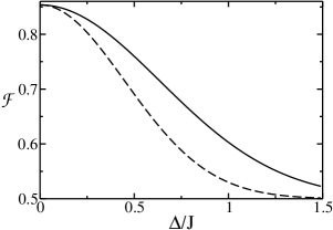
Figure 7: Fidelity for equatorial qubits in the $XY$ model with a classical fluctuating field. $\mathcal{F}$ is plotted as a function of the variance $\Delta$ for fluctuating $J$ (solid) and $B$ (dashed).

However there are situations in which the environment cannot be modeled as classical noise and one has to use a fully quantum mechanical description. Following the standard approach, we model the effects of a quantum environment by coupling the spin network to a bosonic bath. Then we describe the time evolution for the reduced density matrix of the spin system alone, after tracing out the bath degrees of freedom in terms of a master equation cohen . The Hamiltonian for the whole system is

$$H = H_{S}+H_{R}+H_{I}$$ (28)

$$H_{I} = \sum_{i=1}^{M+1}\sum_{k}\lambda_{i}(k)\,\,\sigma_{z}^{i}\left[a_{i}^{\dagger}(k)+a_{i}(k)\right]$$ (29)

$$H_{R} = \sum_{i=1}^{M+1}\sum_{k}\omega_{i}(k)\,\,a_{i}^{\dagger}(k)\,a_{i}(k)$$ (30)

where $H_{S}$ is the spin Hamiltonian defined in Eq. (11). The model is presented for generic $M$ but we will discuss the results only for $M=2$ and $M=3$. We suppose that each spin is coupled to a different bath, labeled by $i$, and that all baths are independent, $\omega_{i}(k)$ and $\lambda_{i}(k)$ are the frequency and the coupling constant of the $k$th mode of the $i$th bath. It is convenient to define the operator $E_{i}=\sum_{k}\lambda_{i}(k)\left[a_{i}^{\dagger}(k)+a_{i}(k)\right]$, the environment operator to which the system is coupled.

The master equation in the basis of eigenstates of $H_{S}$ can be written as:

$$\frac{d}{dt}\rho_{ab}=-\sum_{abcd}\mathcal{R}_{abcd}\,\,\rho_{cd}$$ (31)

where the indexes $a,b,c,d$ run over the energy eigenstates and $\mathcal{R}_{abcd}$ is the so called Bloch-Redfield tensor in the interaction picture:

$${\cal R}_{abcd}=\sum_{i}\int_{0}^{\infty}d\tau\left\{G_{i}(\tau)\Sigma_{abcd}^{>}+G_{i}(-\tau)\Sigma_{abcd}^{<}\right\}$$ (32)

where

$$\Sigma_{abcd}^{>}=\delta_{bd}\sum_{n}(\sigma_{z}^{i})_{an}(\sigma_{z}^{i})_{nc}e^{i\omega_{cn}\tau}-(\sigma_{z}^{i})_{ac}(\sigma_{z}^{i})_{db}e^{i\omega_{ac}\tau}$$ (33)

and

$$\Sigma_{abcd}^{<}=\delta_{ac}\sum_{n}(\sigma_{z}^{i})_{dn}(\sigma_{z}^{i})_{nb}e^{i\omega_{nd}\tau}-(\sigma_{z}^{i})_{ac}(\sigma_{z}^{i})_{db}e^{i\omega_{bd}\tau}$$ (34)

with $(\sigma_{z}^{i})_{ab}=\langle a|\sigma_{z}^{i}|b\rangle$. The function $G(\tau)$ is the correlation function of the environment operators in the interaction picture:

$$G_{i}(\tau)=\text{Tr}\left[\rho_{F}\widetilde{E_{i}}(\tau)\widetilde{E_{i}}(0)\right]$$ (35)

The functions $G_{i}(\tau)$ can be related to the spectral density of the bath through

$$\left[G_{i}(\tau)\right]_{\omega}=2N_{i}(\omega)J_{i}(\omega)$$ (36)

where $\left[\cdot\right]_{\omega}$ indicates the Fourier transform. In Eq.(36) $N_{i}(\omega)=(e^{\beta\omega}-1)^{-1}$ is the mean occupation number of the $\omega_{i}$ mode at temperature $T=\beta^{-1}$ and $J_{i}(\omega)=\pi\sum_{\omega_{k}}\left|\lambda_{i}(\omega_{k})\right|^{2}\delta(\omega-\omega_{k})$ is the spectral density. We suppose that the bath is Ohmic, as often encountered in several situations, i.e. $J(\omega)$ has a simple linear dependency at low frequencies up to some cut-off:

$$J_{i}(\omega)=\frac{\pi}{2}\alpha\omega e^{-\omega/\omega_{C}}$$ (37)

The parameter $\alpha$ represents the strength of the noise and $\omega_{C}$ is the cut-off frequency.

In order to to compare SNC with traditional quantum cloning machines we have to consider a specific system where the required gates are performed. Obviously this can be done in several different ways: we choose the $XY$ Hamiltonian as the model system for both schemes. In particular we compare the two methods for $M=2$ and $M=3$ equatorial qubits. For the quantum circuit approach quantum gates are implemented by a time dependent Hamiltonian. It has been shown kempe02 ; jens that the $XY$ Hamiltonian is sufficient to implement both one and two-qubit gates. The elementary two-qubit gate is the iSWAP:

$$U(iSWAP)=\left(\begin{array}[c]{cccc}1&&&\\ &0&i&\\ &i&0&\\ &&&1\end{array}\right)$$ (38)

It can be obtained turning on an $XY$ interaction between the two qubits without external magnetic field and letting them interact for $Jt=\pi/4$. By applying the iSWAP gate twice, the CNOT operation can be constructed

Figure 8: Circuit implementing the CNOT from the iSWAP. This circuit is used to implement the quantum cloning by means of gates.

This means that we need two two-qubit operations for each CNOT. We simulated the circuits shown in Fig. 1 for $M=2$ and $M=3$ in the presence of noise and we calculated the corresponding fidelities. We neglected the effect of noise during single qubit operations. This is equivalent to assume that the time needed to perform this gates is much smaller than the typical decoherence time. The results are shown in Fig.9 and Fig.10. The fidelity for the quantum gates (squares) and that for the SNC (circles) are compared as functions of the coupling parameter $\alpha$.

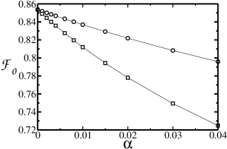
Figure 9: $1\to 2$ cloning. Comparison of the fidelity $\mathcal{F}_{0}$ obtained by the spin network method and the quantum circuit ($XY$ interaction) discussed in du ; buzek97 in the presence of an external quantum noise. Circles and squares refer to the network and gates case respectively ($\vartheta=\pi/2$.). The parameters for the environment are $\beta=10/J$ and $\omega_{C}=10^{4}J$.

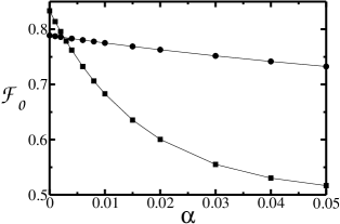
Figure 10: The same as in Fig.9 for the $1\to 3$ case.

Even for small $\alpha$ the fidelity for the circuits is much worse than that for the network. Notice that for $M=3$, though without noise ($\alpha=0$) the SNC fidelity is lower than the ideal one, for $\alpha>\alpha^{*}=2.5\cdot 10^{-3}$ the situation is reversed. This shows that our scheme is more efficient than the one based on quantum gates. Moreover for $M>3$ the time required for quantum circuit PCC grows with increasing M while, as discussed previously, the optimal $t^{(M)}$ of the SNC decreases with $M$. This suggests that our proposal is even more efficient for growing $M$. Changing the model does not affect these results. Indeed the time required to perform a CNOT using Heisenberg or Ising interactions is just half the time required for the $XY$ model.

We also believe that in a real implementation the effect of noise on our system can be very small compared to the that acting on a quantum circuit. This is because during the evolution the spin network can be isolated from the environment.

VII The universal cloner with spin networks

It would be desirable to implement also a universal quantum cloner by the same method illustrated here. In this section we briefly report our attempt to implement the $1\to 2$ universal cloner. In the previous sections we demonstrated that for the models presented the fidelity is invariant on $\varphi$ (phase covariance) but still depends on $\vartheta$. This axial symmetry relies on the selection of the $z$-axis for the initialization of the blank spins. In order to perform a universal cloner we need a spherical symmetry. This means that both the Hamiltonian and the initial state must be isotropic. The first condition is fulfilled using the Heisenberg interaction without static magnetic field that would break the spherical symmetry. The second requirement can be obtained using for the initial state of the blank qubits a completely random state. In other words the complete state of the network (initial state + blanks) is

$$\rho(0)=|\psi\rangle\langle\psi|\otimes\frac{1}{4}\mbox{$1{\bf l}$ }\;\;.$$

The maximum fidelity is obtained for $Jt=\frac{2\pi}{3}$ and has the value

$$\mathcal{F}=13/18\simeq 0.72$$

that has to be compared with the value $5/6\simeq 0.83$ of the optimal universal cloner BH96 . Our model is the most general time independent network containing three spins and fulfills the required conditions.

VIII Quantum cloning of qutrits and qudits

Spin network cloning technique can be generalized to qutrits and qudits. This is what we discuss in this Section starting, for simplicity, with the qutrit case. The cloning of qudits is a straightforward generalization. Our task is to find an interaction Hamiltonian between qutrits able to generate a time evolution as close as possible to the cloning transformation. One obvious generalization of the qubit case is to consider qutrits as spin-1 systems. In this picture the three basis states could be the eigenstates of the angular momentum with z component (-1,0,1). The natural interaction Hamiltonian would then be the Heisenberg or the $XY$ interaction

$$H_{I}=J_{ij}\vec{S^{i}}\cdot\vec{S^{j}}\quad\textrm{or}\quad H_{I}=J_{ij}(S^{i}_{X}S^{j}_{X}+S^{i}_{Y}S^{j}_{Y})$$ (39)

Alternatively one can think to use the state of physical qubits to encode the qutrits. Such an encoding, originally proposed in a different context kempe01 , uses three qubits to encode one single logical qutrit:

$$|0\rangle_{L} = |001\rangle$$

$$|1\rangle_{L} = |010\rangle$$

$$|2\rangle_{L} = |100\rangle$$

In Ref.kempe02 it is shown that this encoding, together with a time-dependent $XY$ interaction, is universal for quantum computing with qutrits. In our work however we have restricted ourselves to the use of time-independent interactions with a suitable design of the spin network. For the qubit case the $XY$ interaction is able to swap two spins. We know that this is the key to clone qubits and so one could try a similar approach also for qutrits. However, for higher spin, Hund’s rule forbids the swapping. For this reason we have turned our attention to the encoded qutrits to see if swapping is possible. It is simple to show that the network depicted in Fig.11 satisfies our requirements.

Figure 11: Arrangement of the network for qutrits. Each dot represents a spin and an ellipse encloses each logical qutrit. A line connecting two dots means that the corresponding spins interact via $XY$ model.

In the arrangement each dot represents a spin and three dots inside an ellipse correspond to an encoded qutrit. A static magnetic field $\Delta$ pointing in the $z$ direction is applied to the first spin. A line connecting two dots means that they interact via an $XY$ interaction with amplitude J. It can be easily checked that for a single couple of qutrits the exchange processes are possible. This network is the generalization of the spin star that we analyzed before in which a single qutrit interacts with the others. It is easily generalized for the $1\to M$ case using three spin stars. The single qutrit Hamiltonian is realized applying magnetic fields to the physical qubits.

In analogy with the qubit cloner we will prepare qutrit 1 in the original state

$$|\psi\rangle=\alpha|0\rangle_{L}+\beta|1\rangle_{L}+\gamma|2\rangle_{L}$$ (40)

and initialize the other qutrits in a blank state, for example $|0\rangle_{L}$. Now due to the interactions the state will evolve in a restricted subspace of the Hilbert space:

$$|\psi(t)\rangle = \alpha|000\rangle_{L}+\beta_{1}|100\rangle_{L}+\beta_{2}|010\rangle_{L}+\beta_{3}|001\rangle_{L}$$ (41)

$$+ \gamma_{1}|200\rangle_{L}+\gamma_{2}|020\rangle_{L}+\gamma_{3}|002\rangle_{L}$$

To find the fidelity of the clones with respect to the state of Eq.(40) we need the reduced density matrix of one of the clones (for example the third). The result, in the basis $(|0\rangle_{L},|1\rangle_{L},|2\rangle_{L})$, is

$$\rho_{3}=\begin{pmatrix}1-\left|\beta_{3}\right|^{2}-\left|\gamma_{3}\right|^{2}&\alpha\beta_{3}^{*}&\alpha\gamma_{3}^{*}\\ \alpha^{*}\beta_{3}&\left|\beta_{3}\right|^{2}&\beta_{3}\gamma_{3}^{*}\\ \alpha^{*}\gamma_{3}&\beta_{3}^{*}\gamma_{3}&\left|\gamma_{3}\right|^{2}\end{pmatrix}$$ (42)

In order to find the coefficients $\beta_{i}(t)$ and $\gamma_{i}(t)$ we have to diagonalize the Hamiltonian. We consider the double PCC of Eq. (7): our model is automatically invariant on $\varphi_{i}$ because there is no preferred direction in the space of the qutrits. The maximum fidelity achievable with SNC is:

$$\mathcal{F}_{3}=\frac{4+2\sqrt{2}}{9}\simeq 0.759$$ (43)

This value has been obtained with $\Delta/J=1/\sqrt{2}$ and $Jt=\pi/\sqrt{2}$. Note that this value is very close to the optimal one and the difference is only $2\cdot 10^{-3}$.

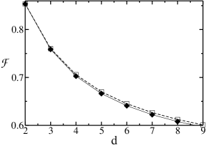
Figure 12: The optimal (square) and the SNC (diamond) fidelities for $1\to 2$ PCC in $d$ dimensions are compared.

We calculated also the fidelity for the $1\to M$ cloning of qutrits using the star configuration. The maximum fidelity is:

$$\mathcal{F}=\frac{2+4\sqrt{M}+3M}{9M}$$ (44)

obtained for the same value of the star configuration of qubits ($Jt^{(M)}=\pi/\sqrt{M}$ and $B^{(M)}/J=\sqrt{M}/2$).

The generalization to qudits is straightforward. Following the same approach we encode qudits using $d$ qubits to encode each qudit. After some algebra one finds the general expression for the PCC in d dimensions. The values $t^{(M)}$ and $B^{(M)}$ are independent from $d$ and the expression for the fidelity is:

$$\mathcal{F}_{1\to 2,d}=\frac{(d-1)(d+2\sqrt{2})+2}{2d^{2}}$$ (45)

In Fig.12 the optimal and SNC fidelities are compared. As we can see, the fidelity of the spin network implementation is very close to the ideal one.

IX Implementation with Josephson nanocircuits

The final section of this work is devoted to the possibility of implementing spin network cloning in solid-state devices. Besides the great interest in solid state quantum information, nanofabricated devices offer great flexibility in the design and allow to realize the graphs represented in Fig.2. We analyze the implementation with Josephson nanocircuits which are currently considered among the most promising candidates as building blocks of quantum information processors schoenreview ; averinreview . Here we discuss only the $1\to 2$ cloning for qubits. The generalization to the other cases is straightforward.

Figure 13: a) A sketch of the charge qubit. It consists of a superconducting electron box formed with an applied gate voltage $V_{x}$. The device operates in the charging regime, i.e. the Josephson couplings $E_{J}$ of the junction (crossed box in the figure) is much smaller than the charging energy. b) Implementation of the $1\to 2$ spin network cloning by means of Josephson qubits. The unknown state to be cloned in stored in the central qubit $c$ while the blank qubits $u$ and $d$ are the ones where the state is cloned. The coupling between the qubits is via the Josephson junctions of coupling energy $J_{K}$.

In the charge regime a Josephson qubit can be realized using a Cooper pair box schoenreview (see Fig.13a), the logical state is characterized by the box having zero or one excess charge. Among the various ways to couple charge qubits, in order to implement SNC the qubits should be coupled via Josephson junctions ourJLTP (see Fig.13b). The central qubit (denoted by $c$ in the figure) will encode the state to be cloned while the upper and lower qubits (denoted with $u$=up and $d$=down) are initially in the blank state. All the Josephson junctions are assumed to be tunable by local magnetic fluxes. The total Hamiltonian of the 3-qubit system is given by the sum of the Hamiltonians of the qubits $H_{0}$ plus the interaction between them $H_{cou}$.

$$H_{0}=\sum_{i=u,c,d}\delta E_{c}\sigma_{z}^{(i)}-E_{J}\sigma_{x}^{(i)}$$ (46)

where $E_{J}$ is the Josephson coupling in the Cooper pair box and $\delta E_{c}$ is the energy difference between the two charge states of the computational Hilbert space. The coupling Hamiltonian for the $3$-qubit system is

$$H_{cou} = \sum_{i=u,d}E_{K}^{(i)}\sigma_{z}^{(c)}\sigma_{z}^{(i)}$$ (47)

$$- (1/2)\sum_{i=u,d}J_{K}^{(i)}[\ \sigma^{(c)}_{+}\sigma^{(i)}_{-}\ +\ \ {\rm h.c.\/}\ ]$$

Here $J_{K}$ is the Josephson energy of the junctions which couple the different qubits and $\sigma_{\pm}=(\sigma_{x}\pm i\sigma_{y})/2$. If the coupling capacitance between the qubits is very small as compared to the other capacitances one can assume $E_{K}^{(j)}$ to be negligible. In practice, however the capacitive coupling is always present therefore it is necessary to have $J_{K}^{(j)}\gg 4E_{K}^{(j)}$. Then the dynamics of the system approximates the ideal $XY$ dynamics required to perform quantum cloning. The protocol to realize the SNC requires the preparation of the initial state. This can be achieved by tuning the gate voltages in such a way that the blank qubits are in $|0\rangle$ and the central qubit is in the state to be cloned. During the preparation the coupling between the qubits should be kept zero by piercing the corresponing SQUID loops of the junctsion $J_{k}$ with a magnetic field equal to a flux quantum. In the second step, $H_{0}$ is switched off and the dynamics of the system is entirely governed by $H_{cou}$. At the optimal time the original state is cloned in the $u$ and $d$ qubits.

Figure 14: Fidelity for the coupling Hamiltonian (47) as a function of $E_{K}/J_{K}$.

As the implementation with superconducting nanocircuits has a slightly different Hamiltonian as compared to the ideal $XY$ model it is important to check for the loss of fidelity due to this difference. As it is shown in Fig.14, for $J_{K}/E_{K}\leq 0.1$ the maximum fidelity achievable differs at most by $\sim 10^{-2}$ from the ideal value.

X Conclusions

We have demonstrated that quantum cloning, in particular PCC, can be realized using no external control but just with an appropriate design of the system Hamiltonian. We considered the Heisenberg and $XY$ coupling between the qubits and we found that the $XY$ model saturates the optimal value for the fidelity of the $1\to 2$ PCC. In all other cases we have analyzed ($N\to M$ PCC, universal cloning, cloning of qudits) our protocol gives a value of the fidelity of clones that is always within a few percent of the optimal value. As compared to the standard protocol using quantum gates, however, there is a major advantage. Our setup is fast and, moreover, its execution time does not increase with the number of qubits to be cloned. In the presence of noise this allows to reach a much better fidelity than the standard protocol even in the presence of a weak coupling to the external environment. In addition we expect that the system in the SNC is better isolated from the external environment because no gate pulses are needed. Finally we proposed a possible implementation of our scheme using superconducting devices available with present day technology. This would be the first experimental realization of quantum cloning in solid state systems. We want to stress that our results on cloning together with others on communication and computation open new perspectives in the realization of a quantum processor, reducing the effect of noise on the system. It would be interesting to consider if it is possible to realize other quantum information protocols or quantum algorithms, using time independent spin networks.

This work was supported by the European Community under contracts IST-SQUIBIT, IST-SQUBIT2, IST-QUPRODIS, IST-SECOQC, and RTN-Nanoscale Dynamics.

References

- (1) W.K. Wootters and W.H. Zurek, Nature 299, 802 (1982).
- (2) N. Gisin and G. Ribordy and W. Tittel and H. Zbinden, Rev. Mod. Phys. 74, 145 (2002).
- (3) V. Bužek and M. Hillery, Phys. Rev. A 54, 1844 (1996).
- (4) E.F. Galvão and L. Hardy, Phys. Rev. A 62, 022301 (2000).
- (5) G. M. D’Ariano and P. Lo Presti, Phys. Rev. A 64, 042308 (2001).
- (6) D. Bruß, D. P. DiVincenzo, A. Ekert, C. A. Fuchs, C. Macchiavello, J. A. Smolin, Phys. Rev. A 57, 2368 (1998).
- (7) N. Gisin and S. Massar, Phys. Rev. Lett. 79, 2153-2156 (1997); D. Bruss, A. Ekert and C. Macchiavello, Phys. Rev. Lett. 81, 2598 (1998); R. F. Werner, Phys. Rev. A58, 1827 (1998).
- (8) D. Bruß, M. Cinchetti, G. M. D’Ariano, C. Macchiavello, Phys. Rev. A 62, 012302 (2000).
- (9) H. K. Cummins, C. Jones, A. Furze, N. F. Soffe, M. Mosca, J. M. Peach, J. A. Jones, Phys. Rev. Lett. 88, 187901 (2002).
- (10) A. Lama-Linares, C. Simon, J.-C. Howell and D. Bouwmeester, Science 296, 712 (2002).
- (11) D. Pelliccia, V. Schettini, F. Sciarrino, C. Sias and F. De Martini, Phys. Rev. A 68, 042306 (2003); F. De Martini, D. Pelliccia and F. Sciarrino, Phys. Rev. Lett. 92, 067901 (2004).
- (12) J. Du, T. Durt, P. Zou, L.C. Kwek, C.H. Lai, C.H. Oh, and A. Ekert, quant-ph/0311010.
- (13) C.-S. Niu and R.B. Griffiths, Phys. Rev. A 60, 2764 (1999).
- (14) S. C. Benjamin and S. Bose, Phys. Rev. Lett. 90, 0247901 (2003).
- (15) M.-H. Yung, D.W. Leung and S. Bose, Quantum Inf. Comput. 4, 174 (2004).
- (16) S. Bose, Phys. Rev. Lett. 91, 207901 (2003).
- (17) V. Subrahmanyam, Phys. Rev. A 69, 034304 (2004).
- (18) T. J. Osborne and N. Linden, Phys. Rev. A 69, 052315 (2004).
- (19) M. Christandl, N. Datta, A. Ekert, and A. J. Landahl, Phys. Rev. Lett. 92, 187902 (2004).
- (20) S. Lloyd, Phys. Rev. Lett. 90, 167902 (2003).
- (21) F. Verstraete, M. A. Martín-Delgado, and J. I. Cirac, Phys. Rev. Lett. 92, 087201 (2004).
- (22) V. Giovannetti and R. Fazio, Phys. Rev. A 71, 032314 (2005).
- (23) A. Romito, R. Fazio and C. Bruder, Phys. Rev. B 71 100501 (2005).
- (24) M. Paternostro, M.S. Kim, G.M. Palma, and G. Falci, Phys. Rev. A 71, 042311 (2005).
- (25) G. De Chiara, R. Fazio, C. Macchiavello, S. Montangero, and G. M. Palma, Phys. Rev. A 70, 062308 (2004).
- (26) G. M. D’Ariano and C. Macchiavello, Phys. Rev. A 67, 042306 (2003).
- (27) A. Olaya-Castro, N. F. Johnson, and L. Quiroga, Phys. Rev. Lett. 94, 110502 (2005).
- (28) There is not a unique formula for arbitrary .
- (29) R. F. Werner, Phys. Rev. A 58, 1827 (1998).
- (30) N.J. Cerf, T. Durt and N. Gisin, J. Mod. Opt., 49, 1355 (2002).
- (31) H. Fan, H. Imai, K. Matsumoto and X.-B. Wang, Phys. Rev. A 67, 022317 (2003)
- (32) F. Buscemi, G. M. D’Ariano and C. Macchiavello, Phys. Rev. A 71, 042327 (2005).
- (33) J. Du, T. Durt, P. Zou, L.C. Kwek, C.H. Lai, C.H. Oh and A. Ekert, Phys. Rev. Lett. 94, 040505.
- (34) V. Bužek, S.L. Braunstein, M. Hillery and D. Bruß, Phys. Rev. A 56, 3446 (1997).
- (35) A. Hutton and S. Bose, Phys. Rev. A 69, 042312 (2002).
- (36) J. Fiurášek, Phys. Rev. A 67, 052314 (2003).
- (37) C. Cohen-Tannoudji, J. Dupont-Rac and G. Grynberg, Atom-Photon Interactions, John Wiley & Sons, New York, (1992)
- (38) J. Kempe and K.B. Whaley, Phys. Rev. A, 65, 052330 (2002).
- (39) N. Schuch and J. Siewert, Phys. Rev. A 67, 032301 (2003).
- (40) J. Kempe, D. Bacon, D. P. DiVincenzo and K.B. Whaley, in Quantum Information and Computation, R. Clark et al. Eds., Rinton Press, New Jersey, Vol.1, 33 (2001).
- (41) Yu. Makhlin, G. Schön, and A. Shnirman, Rev. Mod. Phys. 73, 357 (2001).
- (42) D. V. Averin, Fortschr. Phys. 48, 1055 (2000).
- (43) J. Siewert, R. Fazio, G.M. Palma, and E. Sciacca, J. Low Temp. Phys. 118, 795 (2000).