Exact and approximate many-body dynamics with stochastic one-body density matrix evolution

Abstract

We show that the dynamics of interacting fermions can be exactly replaced by a quantum jump theory in the many-body density matrix space. In this theory, jumps occur between densities formed of pairs of Slater determinants, $D_{ab}=\left|\Phi_{a}\right>\left<\Phi_{b}\right|$, where each state evolves according to the Stochastic Schrödinger Equation (SSE) given in ref. Jul02 . A stochastic Liouville-von Neumann equation is derived as well as the associated Bogolyubov-Born-Green-Kirwood-Yvon (BBGKY) hierarchy. Due to the specific form of the many-body density along the path, the presented theory is equivalent to a stochastic theory in one-body density matrix space, in which each density matrix evolves according to its own mean field augmented by a one-body noise. Guided by the exact reformulation, a stochastic mean field dynamics valid in the weak coupling approximation is proposed. This theory leads to an approximate treatment of two-body effects similar to the extended Time-Dependent Hartree-Fock (Extended TDHF) scheme. In this stochastic mean field dynamics, statistical mixing can be directly considered and jumps occur on a coarse-grained time scale. Accordingly, numerical effort is expected to be significantly reduced for applications.

I Introduction

The purpose of this paper is to discuss the possibility to substitute the description of the evolution of quantum interacting fermions by a stochastic mean-field dynamics of one-body density matrices. In view of present computational capabilities, stochastic methods appear as a promising tool to address exactly or approximately the problem of correlated mesoscopic quantum systems such as nuclei, atomic clusters or Bose-Einstein condensates. Mean field theories, i.e. Hartree-Fock theories, are rarely able to describe the large variety of phenomena occurring in quantum systems. It is generally necessary to extend mean field theory by including the effect of two-body correlations Goe82 . During the past decades, several approximate stochastic theories have been proposed to describe strongly interacting systemsKad62 ; Ayi80 ; Gra81 ; Bal81 ; Ayi88 ; Ayi99 ; Rei92 ; Rei92-2 ; Oni95 . These approaches have in common that the noise is due to the residual part of the interactions acting on top of the mean field. However they generally differ on the strategy used to incorporate noise. In some cases, the residual interaction is treated using statistical assumptions Ayi80 ; Gra81 , while in other cases the interaction induces fluctuations in the wave-packets either by random phase-shifts Bal81 or by quantum jumps according to the Fermi-Golden rule Rei92 ; Oni95 . The influence of correlations is sometimes treated using the notion of stochastic trajectories in the one-body density matrix spaceAyi88 ; Ayi99 . This latter is, among the different theories, the only one that has been applied to large amplitude collective motions in the semi-classical limit Col04 . Recently, its quantal version has been used to describe small amplitude collective vibrations in nuclei Lac01 . However the application of a stochastic approach to the quantum many-body dynamics remains an open problem both from a numerical as well as a conceptual point of view Lac04 ; Lac98-2 .

In this work a different strategy is used to obtain a stochastic formulation of the many-body problem. During the last ten years, many efforts have been made using functional integral techniques Lev80 ; Ker83 ; Neg88 to address the problem of nucleons in strong two-body interactions. These theories provide an exact stochastic formulation of quantum problems and lead to the so-called quantum Monte-Carlo methods Cep95 . Recent applications to nuclear physics have shown that stochastic methods can be applied successfully to describe the structure of nuclei Koo97 . These methods can also be applied to the description of dynamical properties Neg88 . However the self-consistent mean field does not generally play a special role. Indeed the stochastic part is driven either by the kinetic energy part of the Hamiltonian or by a fixed one-body potential in the case of shell model Monte-Carlo calculations Koo97 . Recently a new formulation Car01 ; Jul02 has been proposed that combines the advantages of the Monte-Carlo methods and of the mean field theories. Application of functional integral theories are of great interest since they pave the way to a full implementation of the nuclear static and dynamical many-body problem using mean field theories in a well defined theoretical framework. However the direct application of exact stochastic dynamics to realistic situations remains numerically impossible and proper approximations should be developed.

In the first part of the article, the functional integral method and the associated Stochastic Schroedinger Equation (SSE) developed in Jul02 for many-body and one-body wave functions are presented. The theory is formulated in the more general framework of exact stochastic dynamics in the many-body and/or in the one-body density matrix space. The link between the different formulations is underlined. In a second part, guided by the exact stochastic theory, an extended mean field theory Lac04 taking into account two-body effects in the weak coupling regime is given in terms of a new stochastic one-body evolution.

II Introduction and discussion of stochastic methods

Functional integral methods have been used for a long time to provide a useful reformulation of complex quantum systems Lev80 ; Ker83 (for a review see Neg88 ). This method has been applied with success to describe static properties of nuclei Koo97 . However, it was seldom used for dynamical problems. Recently, an alternative formulation of the path integral representation has been obtained in which the mean field theory plays a specific role. We consider a general many-body system described by the wave function $\left|\Phi\right\rangle$ which evolves according to the Hamiltonian:

$$H=\sum_{ij}T_{ij}a_{i}^{+}a_{j}+\frac{1}{4}\sum_{ijkl}V_{ijkl}a_{i}^{+}a_{j}^{+}a_{l}a_{k},$$ (1)

where the first term corresponds to the kinetic part of the Hamiltonian while the second part is the two-body interaction. We use the convention of Abe96 concerning the labelling of one and two-body operators. We denote $V_{ijkl}=\left\langle ij\left|\widetilde{v}_{12}\right|kl\right\rangle$ where $\widetilde{v}_{12}$ is the antisymmetrized two-body interaction.

II.1 Action of a quadratic Hamiltonian on a Slater determinant

In ref. Koo97 , the general strategy to obtain ground state properties of a many-body system using Monte-Carlo methods is described. The new aspect developed in ref. Jul02 is the introduction a self-consistent mean field before the application of functional integral. In that case, only the residual part of the interaction which is not taken into account in mean field Hamiltonian is treated stochastically. In this section, we summarize how a general two-body Hamiltonian applied to a Slater determinant can be separated into a mean field part and a residual two-body contribution. Details are given in ref. Jul02 .

We consider a Slater determinant $\left|\Phi\right\rangle$ defined as $\left|\Phi\right\rangle=\Pi_{\alpha}a_{\alpha}^{+}\left|0\right\rangle$ , where the single particle states $\left|\alpha\right\rangle$ may not be orthogonal. Starting from the Hamiltonian (1), we have

$$H\left|\Phi\right\rangle=\left(H_{1}+H_{res}\right)\left|\Phi\right\rangle,$$ (2)

with

$$H_{1}\left|\Phi\right\rangle=\left(E_{0}+\sum_{\alpha_{1}\overline{\alpha_{1}}}\left\langle\bar{\alpha}_{1}\left|h_{MF}\left(\rho_{1}\right)\right|\alpha_{1}\right\rangle a_{\bar{\alpha}_{1}}^{+}a_{\hat{\alpha}_{1}}\right)\left|\Phi\right\rangle,$$ (3)

where we denote by $\left|\bar{\alpha}_{1}\right\rangle$ the particle states (i.e. the unoccupied states) and where $\rho_{1}=\sum\left|\alpha_{1}\right\rangle\left\langle\hat{\alpha}_{1}\right|$ is the one-body density associated with $\left|\Phi\right\rangle$. The states $\left|\hat{\alpha}_{1}\right\rangle$ are defined by $\left\langle\hat{\alpha}_{1}\left|{}\right.\alpha_{2}\right\rangle=\delta_{\alpha_{1}\alpha_{2}}$. In this expression, $h_{MF}\left(\rho_{1}\right)$ is the mean field Hamiltonian

$$\begin{array}[]{ll}h_{MF}\left(\rho_{1}\right)&=T_{1}+\overline{v}\left(\rho_{1}\right)\end{array}.$$ (4)

In this equation, $\overline{v}\left(\rho_{1}\right)=Tr_{2}\left(\widetilde{v}_{12}\rho_{2}\right)$ is the mean field potential where $Tr_{2}\left(.\right)$ denotes the partial trace on the second particle. In equation (3), we denote

$$E_{0}=Tr\left(\rho_{1}h_{MF}\left(\rho_{1}\right)-\frac{1}{2}\rho_{1}\overline{v}\left(\rho_{1}\right)\right).$$ (5)

In the single particle basis defined above, it could be shown that

$$\left\langle\bar{\alpha}_{1}\bar{\alpha}_{2}\left|\widetilde{v}_{12}\right|\alpha_{1}\alpha_{2}\right\rangle=-\sum_{s,\alpha_{1}\alpha_{2}\bar{\alpha}_{1}\bar{\alpha}_{2}}\hbar\omega_{s}\left\langle\bar{\alpha}_{1}\left|O_{s}\right|\alpha_{1}\right\rangle\left\langle\bar{\alpha}_{2}\left|O_{s}\right|\alpha_{2}\right\rangle,$$ (6)

where $O_{s}$ is a one-body operator. Note that, the latter transformation of the two-body matrix elements is a particular case of the more general transformations given in ref. Koo97 . When the single particle basis is not the particle-hole state of the Slater determinant, additional terms should be accounted for. Using this transformation, the residual part of the Hamiltonian is

$$H_{res}\left|\Phi\right\rangle=\frac{1}{4}\sum_{s,\alpha_{1}\alpha_{2}\bar{\alpha}_{1}\bar{\alpha}_{2}}\hbar\omega_{s}\left\langle\bar{\alpha}_{1}\left|O_{s}\right|\alpha_{1}\right\rangle\left\langle\bar{\alpha}_{2}\left|O_{s}\right|\alpha_{2}\right\rangle a_{\bar{\alpha}_{1}}^{+}a_{\bar{\alpha}_{2}}^{+}a_{\hat{\alpha}_{1}}a_{\hat{\alpha}_{2}}\left|\Phi\right\rangle.$$ (7)

In next section, this expression is the starting point to derive the stochastic Schroedinger equations using functional integral techniques.

II.2 Functional integrals and stochastic many-body dynamics

Functional integrals methods applied to quantum fermionic systems in interaction Lev80 ; Ker83 lead to general stochastic formulations of the quantum many-body problem. They however also lead to specific difficulties. For instance, the semi-classical limit of the functional integral does not give naturally the Hartree-Fock theory, but only to the Hartree theory. The interesting idea proposed in Jul02 is to use the functional integral already accounting for the fact that the Hamiltonian is applied to a Slater determinant. In this case, only the residual (2 particle-2 hole) part of the Hamiltonian is interpreted as a source of noise. This procedure is summarized now.

We consider the evolution of the system during a small time-step $\Delta t$. Denoting by $\left|\Delta\Phi\right\rangle$ the associated evolution, we have:

$$\left|\Phi+\Delta\Phi\right\rangle=U\left(\Delta t\right)\left|\Phi\right\rangle=\exp\left(\frac{\Delta t}{i\hbar}H\right)\left|\Phi\right\rangle,$$ (8)

where $U\left(\Delta t\right)$ is the propagator associated to $H$. Using the Hubbard-Stratonovitch Hub59 ; Str58 functional integral on the residual part only, the exact propagator transforms into an integral equation Jul02 :

$$\begin{array}[]{ll}U\left(\Delta t\right)\left|\Phi\right\rangle=&\int{d\overrightarrow{{\bf\sigma}}G\left(\overrightarrow{{\bf\sigma}}\right)\exp\left(\frac{\Delta t}{i\hbar}H_{1}+\Delta B\left(\overrightarrow{{\bf\sigma}}\right)\right)\left|\Phi\right\rangle}.\end{array}$$ (9)

$H_{1}$ is given by equation (3) while $\Delta B\left(\overrightarrow{{\bf\sigma}}\right)$ is a one-body operator written as

$$\Delta B\left(\overrightarrow{{\bf\sigma}}\right)\left|\Phi\right\rangle=\sum_{\alpha\bar{\alpha},s}\lambda_{s}\left\langle\overline{\alpha}\left|O_{s}\right|\alpha\right\rangle\Delta W_{s}a_{\bar{\alpha}}^{+}a_{\hat{\alpha}}\left|\Phi\right\rangle,$$ (10)

where

$$\lambda_{s}=\sqrt{\omega_{s}}\left(1+isgn\left(\omega_{s}\right)\right)/2$$ (11)

and $\Delta W_{s}=\sqrt{\Delta t}$ $\sigma_{s}$ with $\sigma_{s}$ the component of the vector $\overrightarrow{{\bf\sigma}}$. In equation (9), $G\left(\overrightarrow{{\bf\sigma}}\right)=\Pi_{s}g(\sigma_{s})$ represents the product of normalized Gaussian probabilities of width $1$ for the $\sigma_{s}$ variables. As in other functional integral formulations, we recover that the original propagator associated to the exact evolution can be replaced by an ensemble of propagators that depend on $\overrightarrow{\sigma}$. Equivalently, in the limit of infinitesimal time step ($\Delta t\longrightarrow dt$), this equation can be interpreted as a stochastic Schroedinger equation for the initial state. Using the standard notation for stochastic processes in Hilbert space Gar85 , we have:

$$\left|\Phi\right\rangle+\left|d\Phi\right\rangle=\exp\left(\frac{dt}{i\hbar}H_{1}+dB\left(t\right)\right)\left|\Phi\right\rangle.$$ (12)

Here $\left|d\Phi\right\rangle$ has to be interpreted as a stochastic wave function. Since eq. (9) is exact, it shows that the exact dynamics of a Slater determinant can be replaced by an average over stochastic evolution operators. In this expression, $dB\left(t\right)$ is a stochastic operator which depends on the stochastic variable $dW_{s}$ according to equation (10). In order to obtain this equation, the Ito rules for stochastic calculus have been used Gar85 with

$$dW_{s_{1}}dW_{s_{2}}=\delta_{s_{1}s_{2}}dt.$$ (13)

Using the latter properties in combination with the expression of $dB\left(t\right)$, we obtain an equivalent of the fluctuation-dissipation theorem that gives the link between the stochastic operator and the residual part of the Hamiltonian:

$$\frac{1}{2}dB\left(t\right)dB\left(t\right)\left|\Phi\right\rangle=+\frac{dt}{i\hbar}H_{res}\left(t\right)\left|\Phi\right\rangle.$$ (14)

Expression (12) is of particular interest. Indeed, according to the Thouless theorem Rin80 ; Bla86 , the application of an operator of the form (12) to a Slater determinant gives another Slater determinant. Therefore, the evolution of correlated systems of fermions can be replaced by stochastic evolutions of an ensemble of Slater determinants. Since each evolution can be solved with numerical techniques used in mean field theories, SSE offer a chance to solve exactly the dynamics of strongly interacting fermionic systems. This property has already been noted in several pioneering works Lev80 ; Ker83 ; Neg88 . A very similar conclusion has been reached for the description of interacting bosons using Monte-Carlo wave function techniques Car01 . In this case and more generally in the context of the stochastic description of open quantum systems, jumps between wave-packets are generally described using differential stochastic dynamics in Hilbert space Ple98 ; Gar00 ; Bre02 . Then, the evolution of $\left|d\Phi\right\rangle$ is directly considered.

The equivalent differential equation associated to the jump process described here can be obtained by developing the exponential in eq. (12) in powers of $dt$. Using Ito rules, we obtain :

$$\left|\Phi\right\rangle+\left|d\Phi\right\rangle=\left(1+\frac{dt}{i\hbar}H_{1}+\frac{1}{2}dB\left(t\right)dB\left(t\right)+dB\left(t\right)\right)\left|\Phi\right\rangle.$$ (15)

Using equations (2) and (14), we finally obtain a stochastic Schroedinger equation for the many-body wave function:

$$\left|d\Phi\right\rangle=\left(\frac{dt}{i\hbar}H+dB\left(t\right)\right)\left|\Phi\right\rangle.$$ (16)

In the following, this equation is referred to as the many-body SSE. Equation (16) is strictly equivalent to (12) and thus preserves the Slater determinant nature of the states along the stochastic trajectory. This might appear surprising due to the appearance of the complete Hamiltonian $H$ in eq. (16). This is a specific aspect of the stochastic many-body theory using Ito stochastic calculus. Indeed, although $H$ (which contains the complete two-body interaction) drives the initial state out from the Slater determinant space, the stochastic part of the equation of evolution compensates this effect exactly. The exponential form (12) or the differential form (16) describe the same stochastic process. However, differential equations are generally easier to manipulate Ple98 ; Gar00 ; Bre02 .

II.3 Equivalent quantum jump for single particle states

Up to now, we have introduced notions associated with the stochastic mechanics of many-body wave functions. This formulation is of great interest for applications since the stochastic evolution of the many-body wave function can be replaced by the stochastic evolution of its single particle components. For completeness the equivalent differential equation of single particle wave function is given below. It has been shown in ref. Jul02 that equation (12) leads to the single particle equation of motion

$$\left|d\alpha\right\rangle=\frac{dt}{i\hbar}h\left(\rho_{1}\right)\left|\alpha\right\rangle+\sum_{s}\lambda_{s}\left(1-\rho_{1}\right)O_{s}\left|\alpha\right\rangle dW_{s},$$ (17)

where $h\left(\rho_{1}\right)$ is a one-body operator given by

$$h\left(\rho_{1}\right)=h_{MF}\left(\rho_{1}\right)-\frac{1}{2}\rho_{1}\overline{v}\left(\rho_{1}\right).$$ (18)

Equation (17) will be referred to as the one-body SSE. We would like to stress again that eq. (16) and the set of single particle evolutions (eq. (17)) are strictly equivalent.

In this section, we have summarized the equivalence between quantum jump approaches in many-body and one-body spaces of wave-packets in order to describe interacting fermions. An equivalent formulation in terms of density matrices is highly desirable to compare the exact treatment with other stochastic methods.

III Density matrix formulation

In the previous section, we have considered the stochastic formulation of the many-body problem using stochastic Schroedinger equation. In this approach, all trajectories start from a Slater determinant and follow a stochastic path in the Slater determinant space. Stochastic theories can also be applied if the system is initially correlated. In this case, it is helpful to generalize the theory by introducing density matrices. It has been shown in ref. Jul02 that the many-body density matrix $D\left(t\right)$ associated with the system at all times can be properly described by the average over an ensemble of pairs of non-orthogonal Slater determinants state vectors,

$$D\left(t\right)=\overline{\left|\Phi_{a}\right\rangle\left\langle\Phi_{b}\right|},$$ (19)

each of them evolving according to eq. (16). Here, the average over the initial ensemble has been introduced. In that case, the notion of a quantum jump between the wave functions is replaced by a quantum jump in the space of Slater determinants pairs. In the following, the properties of Slater-determinant dyadics are recalled and a stochastic BBGKY hierarchy Kir46 ; Bog46 ; Bor46 is derived.

III.1 Slater determinant dyadics: notations

Let us consider a many-body density formed of two distinct Slater determinants

$$D_{ab}=\left|\Phi_{a}\right\rangle\left\langle\Phi_{b}\right|,$$ (20)

in which each Slater determinant is an antisymmetrized product of not necessarily orthogonal single particle states

$$\left\{\begin{array}[]{ll}\left|\Phi_{a}\right\rangle&=\Pi_{\alpha}a_{\alpha}^{+}\left|0\right\rangle\\ \left|\Phi_{b}\right\rangle&=\Pi_{\beta}a_{\beta}^{+}\left|0\right\rangle\end{array}\right..$$ (23)

Note that $D_{ab}$ is neither hermitian nor normalized. However, for convenience we will still call it a density matrix. Starting from the many-body density matrix, one can obtain the generalized $k-$body density matrix (denoted by $\rho_{1\ldots k}$ ) by taking successive partial traces. Using the same notation as in Abe96 , we have:

$$\rho_{1\ldots k}^{(ab)}=Tr_{{}_{k+1\ldots,A}}\left(D_{ab}\right),$$ (24)

where $A$ is the size of the system. One can obtain the expression of density matrices in terms of single particle states of the two Slater determinants by introducing the overlap matrix elements between single particle states, denoted by $f$. The matrix elements of $f$ are defined by $f_{\beta_{i}\alpha_{j}}=\left\langle\beta_{i}|\alpha_{j}\right\rangle$. For instance, the one-body density matrix is:

$$\rho_{1}^{(ab)}={\it\ }\det\left(f\right)\sum_{\alpha_{i}\beta_{j}}\left|\alpha_{i}\right\rangle f_{\alpha_{i}\beta_{j}}^{-1}\left\langle\beta_{j}\right|\equiv\det\left(f\right)u_{1}^{\left(ab\right)}.$$ (25)

More generally the $k-$body density matrix is the antisymmetrized product of single particle densities Low55

$$\rho_{1,\ldots,k}^{(ab)}=\det\left(f\right){\cal A}\left(u_{1}^{(ab)}\ldots u_{k}^{\left(ab\right)}\right),$$ (26)

where ${\cal A}\left(.\right)$ corresponds to the antisymmetrization operator. Introducing the two-body correlation operator defined by

$$C_{12}^{(ab)}=\rho_{12}^{(ab)}-{\cal A}\left(u_{1}^{(ab)}\rho_{2}^{(ab)}\right),$$ (27)

we have $C_{12}^{(ab)}=0$ for any state defined by equation (20).

III.2 Stochastic evolution of many-body density matrices

The BBGKY hierarchy Kir46 ; Bog46 ; Bor46 has been widely used as a starting point in order to obtain approximations Abe96 on the evolution of complex systems. Therefore, an equivalent hierarchy associated to the exact stochastic mean field deduced from functional integrals is highly desirable to specify the possible links with other theories. In this section, starting from the stochastic Schroedinger equation for the many-body wave function, we give the associated stochastic formulation of the BBGKY hierarchy. In the stochastic many-body dynamics, we consider the quantum jump between two different density matrices $D_{ab}$ and $D_{ab}^{\prime}$. Starting from $D_{ab}$ given by eq. (20), there are transitions towards another density matrix given by $D_{ab}^{\prime}=\left|\Phi_{a}+d\Phi_{a}\right\rangle\left\langle\Phi_{b}+d\Phi_{b}\right|$. The rules for transitions are directly obtained from the rules for the jumps in the wave functions space:

$$\left\{\begin{array}[]{rr}\left|d\Phi_{a}\right\rangle&=\frac{dt}{i\hbar}H\left|\Phi_{a}\right\rangle+dB_{a}\left|\Phi_{a}\right\rangle\\ \left\langle d\Phi_{b}\right|&=-\frac{dt}{i\hbar}\left\langle\Phi_{b}\right|H+\left\langle\Phi_{b}\right|dB_{b}^{+}.\end{array}\right.$$ (30)

with

$$\begin{array}[]{rr}dB_{a}&=\sum_{s}\lambda_{s}\sum_{\hat{\alpha}\overline{\alpha}}a_{\overline{\alpha}}^{+}\left\langle\overline{\alpha}\left|O_{s}\right|\alpha\right\rangle a_{\hat{\alpha}}dW_{s_{a}}\\ dB_{b}^{+}&=\sum_{s}\lambda_{s}^{\ast}\sum_{\hat{\beta}\overline{\beta}}a_{\hat{\beta}}^{+}\left\langle\beta\left|O_{s}\right|\overline{\beta}\right\rangle a_{\overline{\beta}}dW_{s_{b}}.\end{array}$$ (33)

The notation $dW_{s_{a}}$ and $dW_{s_{b}}$ are introduced in order to emphasize that stochastic variables associated respectively to $\left|\Phi_{a}\right\rangle$ and $\left|\Phi_{b}\right\rangle$ are statistically independent, i.e.

$$dW_{s_{a}}dW_{s_{b}}=0.$$ (34)

This complete eq. (13) verified both by $dW_{s_{a}}$ and $dW_{s_{b}}$. With these rules, the evolution of the many-body density matrix along the stochastic path is given by

$$dD_{ab}=\frac{dt}{i\hbar}\left[H,D_{ab}\right]+dB_{a}D_{ab}+D_{ab}dB_{b}^{+}.$$ (35)

This equation is a stochastic version of the Liouville-von Neumann equation for the density matrix. The evolution of the $k-$body density matrix can be directly derived from expression (35) and one obtains:

$$d\rho_{1\ldots k}^{(ab)}=\frac{dt}{i\hbar}Tr_{k+1,\ldots,A}\left(\left[H,D_{ab}\right]\right)+d{\cal W}_{ab}^{k}.$$ (36)

The additional term corresponds to the stochastic part acting on the $k$-body density matrix evolution:

$$d{\cal W}_{ab}^{k}=Tr_{k+1,\ldots,A}\left(dB_{a}D_{ab}+D_{ab}dB_{b}^{+}\right).$$ (37)

The first part of eq. (36) is nothing but the standard expression of the $k^{th}$ equation of the BBGKY hierarchy whose explicit form can be found in review articles Cas90 ; Rei94 ; Abe96 . The equation of motion for the $k-$body density matrix in the framework of the stochastic many-body theory proposed in ref. Jul02 corresponds to the standard BBGKY term augmented by a one-body stochastic noise.

III.3 Evolution of the one-body density matrix

Starting from (36), an explicit form of the one-body density evolution can be found. Since for any $D_{ab}$, we have $C^{(ab)}_{12}=0$, the first term in eq. (36) reduces to:

$$\begin{array}[]{ll}Tr_{2\ldots,A}\left(\left[H,D_{ab}\right]\right)&=Tr_{2}\left(\left[H,\rho_{12}^{(ab)}\right]\right)\\ &=\left[h_{MF}\left(u_{1}^{(ab)}\right),\rho_{1}^{(ab)}\right].\end{array}$$ (38)

The stochastic part reads:

$$\begin{array}[]{ll}Tr_{2,\ldots,A}\left(dB_{a}D_{ab}\right)=&\sum_{s}\lambda_{s}\sum_{\alpha\bar{\alpha}}\left\langle\bar{\alpha}\left|O_{s}\right|\alpha\right\rangle\\ &\times Tr_{2,\ldots,A}\left(a_{\bar{\alpha}}^{+}a_{\hat{\alpha}}D_{ab}\right)dW_{s_{a}}.\end{array}$$ (41)

Let us introduce a complete single particle basis. For any state $\left|i\right\rangle$ and $\left|j\right\rangle$ of the basis, we have :

$$\begin{array}[]{ll}\left\langle i\left|Tr_{2,\ldots,A}\left(a_{\bar{\alpha}}^{+}a_{\hat{\alpha}}D_{ab}\right)\right|j\right\rangle&=Tr\left(a_{j}^{+}a_{i}a_{\bar{\alpha}}^{+}a_{\hat{\alpha}}D_{ab}\right)\\ &=\sum_{kl}\left\langle k\left|{}\right.\bar{\alpha}\right\rangle\left\langle\hat{\alpha}\left|{}\right.l\right\rangle Tr\left(a_{j}^{+}a_{i}a_{k}^{+}a_{l}D_{ab}\right).\end{array}$$ (42)

Using the fermionic commutation rules on creation/annihilation operators together with the definition of the one- and two-body density matrices, we obtain:

$$\begin{array}[]{ll}\left\langle i\left|Tr_{2,\ldots,A}\left(a_{\bar{\alpha}}^{+}a_{\hat{\alpha}}D_{ab}\right)\right|j\right\rangle&=\sum_{kl}\left\langle k\left|{}\right.\bar{\alpha}\right\rangle\left\langle\hat{\alpha}\left|{}\right.l\right\rangle\left\langle li\left|\rho_{12}^{(ab)}\right|kj\right\rangle\\ &+\sum_{l}\left\langle i\left|{}\right.\bar{\alpha}\right\rangle\left\langle\hat{\alpha}\left|{}\right.l\right\rangle\left\langle l\left|\rho_{1}^{\left(ab\right)}\right|j\right\rangle.\end{array}$$ (43)

Using the fact that $\rho_{12}={\cal A}\left(u_{1}\rho_{2}\right)$, we finally obtain:

$$\begin{array}[]{r}Tr_{2,\ldots,A}\left(dB_{a}D_{ab}\right)=\sum_{s}\lambda_{s}\left(1-u_{1}^{(ab)}\right)O_{s}\rho_{1}^{(ab)}dW_{s_{a}}\\ +\sum_{s}\lambda_{s}Tr\left(u_{1}^{(ab)}\left(1-\rho_{a}\right)O_{s}\right)\rho_{1}^{(ab)}dW_{s_{a}},\end{array}$$ (46)

where the one-body density $\rho_{a}$ associated with $\left|\Phi_{a}\right\rangle$ has been introduced. The same treatment can be performed for the second part of the stochastic term and the evolution of the one-body density matrix finally reads:

$$d\rho_{1}^{(ab)}=$$ ,

(47)

with

$$\begin{array}[]{ll}db_{1}^{(ab)}=&\sum_{s}\lambda_{s}\left(1-u_{1}^{(ab)}\right)O_{s}\rho_{1}^{(ab)}dW_{s_{a}}+\sum_{s}\lambda_{s}Tr\left(u_{1}^{(ab)}\left(1-\rho_{a}\right)O_{s}\right)\rho_{1}^{(ab)}dW_{s_{a}}\\ &+\sum_{s}\lambda_{s}^{\ast}\rho_{1}^{(ab)}O_{s}\left(1-u_{1}^{(ab)}\right)dW_{s_{b}}+\sum_{s}\lambda_{s}^{\ast}Tr\left(O_{s}\left(1-\rho_{b}\right)u_{1}^{(ab)}\right)\rho_{1}^{(ab)}dW_{s_{b}}.\end{array}$$ (48)

It is interesting to note that although the single particle states entering in $\rho_{1}^{(ab)}$ do not evolve according to mean field theory but according to $h\left(\rho_{1}^{(ab)}\right)$ given by (18), the deterministic part associated with the evolution of the one-body density reduces to the standard mean field propagation. Eq. (47) points out the central role played by the mean field Hamiltonian in the stochastic many-body theory. In particular, it shows that any evolution of a correlated physical system submitted to a two-body interaction can be replaced by a set of mean field evolutions augmented by a one-body noise. Finally, it is worth noticing that expression  (47) can alternatively be obtained by differentiating directly $\rho_{1}^{(ab)}=\det\left(f\right)\sum_{\alpha_{i}\beta_{j}}\left|\alpha_{i}\right\rangle f_{\alpha_{i}\beta_{j}}^{-1}\left\langle\beta_{j}\right|$.

III.4 k-body density evolution from one-body density

The stochastic evolution transforms a pair of Slater determinants into another pair of Slater determinants. Thus, all the information on a single stochastic trajectory is contained in the stochastic evolution of the one-body density evolution in eq. (47). Indeed, the evolution of the $k-$body density matrix can be directly obtained from the relation (26) which is valid all along the stochastic path. Using the Ito rules, we have

$$\begin{array}[]{ll}d\rho_{1\ldots k}^{(ab)}=&d\left(\det\left(f\right)\right){\cal A}\left(u_{1}^{\left(ab\right)}\ldots u_{k}^{\left(ab\right)}\right)\\ &+\det\left(f\right)\sum_{i}{\cal A}\left(u_{1}^{\left(ab\right)}\ldots du_{i}^{\left(ab\right)}\ldots u_{k}^{\left(ab\right)}\right)\\ &+d\left(\det\left(f\right)\right)\sum_{i}{\cal A}\left(u_{1}^{\left(ab\right)}\ldots du_{i}^{\left(ab\right)}\ldots u_{k}^{\left(ab\right)}\right)\\ &+\det\left(f\right){\cal A}\left(\sum_{i\neq j}u_{1}^{\left(ab\right)}\ldots du_{i}^{\left(ab\right)}\ldots du_{j}^{\left(ab\right)}\ldots u_{k}^{\left(ab\right)}\right).\end{array}$$ (49)

It can be checked that the terms which are linear in $dt$ correspond to the deterministic part of eq. (36). The latter expression is also useful in order to have an explicit form of the stochastic noise to all order in $k$. In expression (49), $d\left(\det\left(f\right)\right)$ is deduced from equations (30). We have

$$d\det(f) = \left<d\Phi_{b}\left|\right.\Phi_{a}\right>+\left<\Phi_{b}\left|\right.d\Phi_{a}\right>$$ (50)

$$= \left<\Phi_{b}\left|dB_{a}+dB^{+}_{b}\right|\Phi_{a}\right>,$$ (51)

which gives

$$d\det\left(f\right)=\sum_{s}\lambda_{s}Tr\left(u^{(ab)}_{1}\left(1-\rho_{a}\right)O_{s}\right)dW_{s_{a}}+\sum_{s}\lambda_{s}^{\ast}Tr\left(O_{s}\left(1-\rho_{b}\right)u^{(ab)}_{1}\right)dW_{s_{b}}.$$ (52)

In addition, the equation on $du_{i}^{\left(ab\right)}$ is deduced from (47). Altogether, we obtain

$$\begin{array}[]{ll}d{\cal W}_{ab}^{k}=&\sum_{i,s}\lambda_{s}\left[\left(1-u_{i}^{\left(ab\right)}\right)O_{s}^{i}\right]dW_{s_{a}}\rho_{1\ldots k}^{\left(ab\right)}\\ &+\rho_{1\ldots k}^{\left(ab\right)}\sum_{i,s}\lambda_{s}^{\ast}\left[O_{s}^{i}\left(1-u_{i}^{\left(ab\right)}\right)\right]dW_{s_{a}}\\ &+\sum_{s}\lambda_{s}Tr\left(u_{1}^{\left(ab\right)}\left(1-\rho_{a}\right)O_{s}\right)dW_{s_{a}}\rho_{1\ldots k}^{\left(ab\right)}\\ &+\sum_{s}\lambda_{s}^{\ast}Tr\left(O_{s}\left(1-\rho_{b}\right)u_{1}^{\left(ab\right)}\right)dW_{s_{b}}\rho_{1\ldots k}^{\left(ab\right)}.\end{array}$$ (53)

Here, we introduced the notation $O^{i}_{s}$ to denote that the one-body operator $O_{s}$ is applied to the particle $"i"$. The possibility to derive the evolution of $\rho_{1\ldots k}$ for all $k$ from the evolution of $\rho_{1}$ is an illustration of an attractive aspect of this theory. Indeed, since we are considering pairs of Slater determinants, all the information on the dynamics is contained in their one-body densities. This proves that the exact evolution of the density matrix of a correlated system through a two-body Hamiltonian can always be replaced by the average evolution of uncorrelated states each of them evolving in the one-body space according to its own mean field augmented by a one-body stochastic noise.

III.5 Summary

Functional integral methods are attractive since they provide a rather transparent and systematic way of transforming the exact dynamics of a correlated system into a stochastic mean field dynamics. In this work, we have discussed the link between the different one-body and many-body SSE’s on one side and the stochastic one-body and many-body density evolution on the other side. The equivalence and the relationship between the various ways of considering stochastic mechanics are displayed in fig. 1.

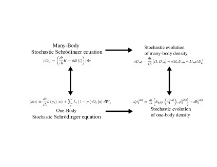
Figure 1: Summary of the four different ways of considering the exact reformulation of the quantum many-body problem using stochastic mechanics. The single arrow indicates that the density matrix formulation can be derived from the stochastic Schroedinger equations. The double arrows show that for both wave function or density matrix formulations, there is a strict equivalence between the many-body and the one-body stochastic equation of motion.

The exact stochastic formulation of the dynamics of complex systems provides a well defined framework to introduce stochastic theories. However, the stochastic dynamics as it is proposed is still rather cumbersome as far as numerical applications are concerned. Indeed, due to the increasing number of trajectories with the number of degrees of freedom, exact stochastic many-body theories have only been applied to dynamics of rather schematic modelsJul02 . With present computational facilities, there is no chance to apply the exact theory to realistic mesoscopic systems and approximate formulations are necessary. The stochastic theory provides however a natural way to replace the dynamics of an interacting system by one-body dynamical evolutions. In the following, we will transform the stochastic equation to account approximately for the correlation and reduce the numerical effort.

IV Approximate stochastic many-body dynamics

A number of approximations of the many-body problem can be found in the literature. Among them, the mean field theory is certainly the most widely used. Correlations beyond the mean field are often required to have a realistic description of dissipative aspects in mesoscopic systems. A general strategy to obtain extensions of the mean field dynamics consists in performing successive truncations of the BBGKY hierarchyCas90 ; Sur95 ; Lac04 . The first order truncation of the hierarchy leads for instance to the standard mean field theory. An extension of the mean field can be obtained by considering the first and second equations of the hierarchy. This has led to different levels of approximations to the nuclear many-body problem as for instance the so-called extended Time-Dependent Hartree-FockWon78 ; Orl79 ; Toh87 (for a recent review see ref. Lac04 ). In the following, we will show that the stochastic evolution described previously can be adapted to a stochastic one-body theory for correlated systems equivalent to the extended TDHF.

IV.1 Extended mean field dynamics

Theories beyond mean field Wei80 ; Cas90 are valid when the dynamical effect of the residual interaction is weak. In the weak coupling regime, correlations can be treated perturbatively on top of the mean field. These theories are valid under the assumption that different time scales associated respectively to two-body collisions and to the mean field propagation exist. Consider $\tau_{coll}$ the time scale for an in-medium two-body collision, and $\tau_{free}$ the time between two collisions. In the weak coupling approximation, one can assume that there exists a time interval $\Delta t$ verifying the condition

$$\tau_{coll}\ll\Delta t\ll\tau_{free}.$$ (54)

An estimate and a discussion of these time scales can be found in ref. Wei80 ; Kol95 . The physical picture to interpret the separation of time scales is that each single particle state evolves according to the average mean field and rarely ”encounters” a two-body collision. From the many-body problem point of view, the role of the residual part of the interaction is to account for two-body collisions.

Besides time scales, extended TDHF remains a one-body theory. Indeed, it is assumed that part of the two-body correlations can be neglected and that the two-body density matrix can be instantaneously approximated by an antisymmetrized product of one-body density matrices ($\rho_{12}(t)={\cal A}\left[\rho_{1}(t)\rho_{2}(t)\right]$). This is of special interest for practical applications since only one-body degrees of freedom are followed in time.

IV.2 Approximate stochastic dynamics

In this section, we propose a formulation of extended one-body dynamics in terms of quantum jumps in the space of one-body density using the same hypothesis as in extended TDHF. We start from a system described at time $t_{0}$ by its one-body density given by

$$\rho_{1}\left(t_{0}\right)=\sum_{\alpha}\left|\alpha\right\rangle n_{\alpha}\left\langle\alpha\right|.$$ (55)

The system is assumed to be initially uncorrelated so that $\rho_{12}\left(t_{0}\right)={\cal A}\left(\rho_{1}\left(t_{0}\right)\rho_{2}\left(t_{0}\right)\right)$. Let us now consider an ensemble of one-body density matrices, noted $\rho^{(n)}_{1}$ with initial conditions $\rho^{(n)}_{1}(t_{0})=\rho_{1}\left(t_{0}\right)$. The time interval $\Delta t$ is divided into $N$ time steps ($\Delta t=N\Delta s$) and at each time step, $\rho^{(n)}_{1}$ evolves according to its mean field augmented by a stochastic term

$$\Delta\rho^{(n)}_{1}=\frac{\Delta s}{i\hbar}\left[h_{MF}\left(\rho^{(n)}_{1}\right),\rho^{(n)}_{1}\right]+\Delta K\left(\rho^{(n)}_{1}\right).$$ (56)

However, contrary to the strategy of the previous section, and following the hypothesis of extended mean field theory, jumps are supposed to occur only once in the time interval $\Delta t$. For a jump occurring at a time $\tau=k\Delta s$, the stochastic term is written as

$$\begin{array}[]{lll}\Delta K\left(\rho^{(n)}_{1}\left(t\right)\right)=\delta_{t,\tau}&&\left\{\sum_{s}\lambda_{s}\left(1-\rho^{(n)}_{1}\left(t\right)\right)O_{s}\rho^{(n)}_{1}\left(t\right)\Delta W_{s}\right.\\ &&\left.+\sum_{s^{\prime}}\lambda_{s^{\prime}}^{\ast}\rho^{(n)}_{1}\left(t\right)O_{s}\left(1-\rho^{(n)}_{1}\left(t\right)\right)\Delta W_{s^{\prime}}\right\},\end{array}$$ (59)

where $\lambda_{s}$ and $O_{s}$ are defined in previous section, while $\Delta W_{s}$ and $\Delta W_{s^{\prime}}$ are two independent Gaussian stochastic variables that follow Ito stochastic rules, with

$$\begin{array}[]{lll}\overline{\Delta W_{s_{1}}\Delta W_{s_{2}}}&=&\delta_{s_{1}s_{2}}\Delta s\\ \overline{\Delta W_{s^{\prime}_{1}}\Delta W_{s^{\prime}_{2}}}&=&\delta_{s^{\prime}_{1}s^{\prime}_{2}}\Delta s.\end{array}$$ (62)

We consider the ensemble of trajectories with a quantum jump occurring at a specific time $\tau$. $\overline{\rho^{\tau}_{12}}(t)$ denotes the two-body density obtained by averaging ${\cal A}\left[\rho^{(n)}_{1}\rho^{(n^{\prime})}_{2}\right]$ over these trajectories.

Before the time $\tau$, all trajectories follow the same path corresponding to the mean field propagation with the initial condition $\rho_{1}\left(t_{0}\right)$. We note respectively $\rho^{mf}_{1}$ and $U_{mf}$ the associated one-body density and propagator. We have

$$\rho^{mf}_{1}(t^{\prime})=U_{mf}\left(t^{\prime},t_{0}\right)\rho_{1}\left(t_{0}\right)U^{+}_{mf}\left(t^{\prime},t_{0}\right),$$ (63)

with

$$U_{mf}\left(t^{\prime},t_{0}\right)=T\exp\left(+\frac{1}{i\hbar}\int_{t_{0}}^{t^{\prime}}h_{mf}\left(\rho^{mf}_{1}\left(s\right)\right)ds\right).$$ (64)

Using these definitions, the evolution between $\tau$ and $\tau+\Delta s$ of the product $\left(\rho^{(n)}_{1}\rho^{(n^{\prime})}_{2}\right)$ is

$$\Delta\left(\rho^{(n)}_{1}\rho^{(n^{\prime})}_{2}\right)=\left(\Delta\rho^{(n)}_{1}\right)\rho^{(n^{\prime})}_{2}+\rho^{(n)}_{1}\left(\Delta\rho^{(n^{\prime})}_{2}\right)+\left(\Delta\rho^{(n)}_{1}\right)\left(\Delta\rho^{(n^{\prime})}_{2}\right).$$ (65)

Using expression (56) and Ito rules, we obtain

$$\begin{array}[]{lll}\Delta\rho^{(n)}_{1}\rho^{(n^{\prime})}_{2}(\tau)&=&\frac{\Delta s}{i\hbar}\left[h_{mf}\left(\rho^{mf}_{1}(\tau)\right)+h_{mf}\left(\rho^{mf}_{2}(\tau)\right),\rho^{mf}_{1}(\tau)\rho^{mf}_{2}(\tau)\right]\\ &&+\Delta K\left(\rho^{(n)}_{1}\right)\Delta K\left(\rho^{(n^{\prime})}_{2}\right)+\Delta K\left(\rho^{(n)}_{1}\right)+\Delta K\left(\rho^{(n^{\prime})}_{2}\right).\end{array}$$ (68)

We have used the fact that, for all considered trajectories, no collision occurs before time $\tau$ leading to $\rho^{(n)}_{1}(\tau)=\rho^{(n^{\prime})}_{1}(\tau)=\rho^{mf}_{1}(\tau)$. The last two terms of equation (68) do not contribute to the average evolution. We thus see that, in addition to the mean field, an extra deterministic term will appear in the average evolution (68). Using equations (62),we have

$$\begin{array}[]{lll}\overline{\Delta K\left(\rho^{(n)}_{1}\right)\Delta K\left(\rho^{(n^{\prime})}_{2}\right)}&=&\Delta s\sum_{s}(\lambda_{s})^{2}\left(1-\rho^{mf}_{1}\left(\tau\right)\right)\left(1-\rho^{mf}_{2}\left(\tau\right)\right)O^{1}_{s}O^{2}_{s}\rho^{mf}_{1}\left(\tau\right)\rho^{mf}_{2}\left(\tau\right)\\ &+&\Delta s\sum_{s}(\lambda^{*}_{s})^{2}\rho^{mf}_{1}\left(\tau\right)\rho^{mf}_{2}\left(\tau\right)O^{1}_{s}O^{2}_{s}\left(1-\rho^{mf}_{1}\left(\tau\right)\right)\left(1-\rho^{mf}_{2}\left(\tau\right)\right).\end{array}$$ (71)

Using finally the fact that $\lambda^{2}_{s}=i\omega_{s}/2$, relation (6) and introducing the antisymmetrization operators, we obtain the average evolution

$$\overline{\Delta{\cal A}\left(\rho^{(n)}_{1}\rho^{(n^{\prime})}_{2}\right)(\tau)}=\frac{\Delta s}{i\hbar}\left[h_{mf}\left(\rho^{mf}_{1}(\tau)\right)+h_{mf}\left(\rho^{mf}_{2}(\tau)\right),{\cal A}\left(\rho^{mf}_{1}(\tau)\rho^{mf}_{2}(\tau)\right)\right]+\frac{\Delta s}{i\hbar}F_{12}\left(\tau\right).$$ (72)

In this equation, $F_{12}$ reads

$$\begin{array}[]{lll}F_{12}(\tau)&=&\left(1-\rho^{mf}_{1}\left(\tau\right)\right)\left(1-\rho^{mf}_{2}\left(\tau\right)\right)\widetilde{v}_{12}\rho^{mf}_{1}\left(\tau\right)\rho^{mf}_{2}\left(\tau\right)\\ &&-\rho^{mf}_{1}\left(\tau\right)\rho^{mf}_{2}\left(\tau\right)\widetilde{v}_{12}\left(1-\rho^{mf}_{1}\left(\tau\right)\right)\left(1-\rho^{mf}_{2}\left(\tau\right)\right).\end{array}$$ (75)

As discussed in Lac98-2 , the effect of a single collision is expected to be weak during the time interval $\Delta t$ and we can assume that for all trajectories, the mean field propagation coincides with $U_{mf}$ after the jump. Therefore, the average density at the final time $t_{f}=t_{0}+\Delta t$ is given by:

$$\overline{\rho^{\tau}_{12}}(t_{f})={\cal A}\left(\rho_{1}^{mf}(t_{f})\rho_{2}^{mf}(t_{f})\right)+\frac{\Delta s}{i\hbar}U^{12}_{mf}\left(t_{f},\tau\right)F_{12}\left(\tau\right)U^{12+}_{mf}\left(t_{f},\tau\right),$$ (76)

where $U^{12}_{mf}=U^{1}_{mf}\otimes U^{2}_{mf}$. The complete average density $\overline{\rho_{12}}(t_{f})$ is obtained by summing different possible times $\tau$ for collisions:

$$\overline{\rho_{12}}(t_{f})={\cal A}\left(\rho^{mf}_{1}(t_{f})\rho^{mf}_{2}(t_{f})\right)+\frac{1}{i\hbar}\int_{t_{0}}^{t_{f}}dsU^{12}_{mf}\left(t_{f},s\right)F_{12}\left(s\right)U^{12+}_{mf}\left(t_{f},s\right),$$ (77)

where the limit $\Delta s\rightarrow ds$ has been taken. This two-body density matrix corresponds to the standard mean field propagation augmented by the incoherent contribution of nucleon-nucleon collisions entering generally in extended mean field theories Lac04 .

As mentioned previously, an interesting aspect of extended TDHF is that it contains only one-body degrees of freedom. This can only be achieved by projecting correlation effects in the single particle space. In the stochastic dynamics presented here, this is equivalent to assume that the final two-body density can be approximated by ${\cal A}\left(\rho_{1}(t_{f})\rho_{2}(t_{f})\right)$ where $\rho_{1}(t_{f})$ is given by

$$\rho_{1}(t_{f})=Tr_{2}\left(\overline{\rho_{12}}\left(t_{f}\right)\right).$$ (78)

The density obtained in this way differs from the density propagated by the mean field alone and contains the effect of incoherent nucleon-nucleon collisions. The procedure can then be iterated using the new density as a starting point for future stochastic propagation.

In this section, we have presented a method to include approximately two-body effects by means of a stochastic one-body theory. As in the exact formulation presented in the previous section, the stochastic theory can be equivalently formulated as a stochastic Schroedinger equation. It is important to note that the numerical effort required for the approximate dynamics is expected to be much less than for the exact one at least for two reasons. The first one comes from the fact that quantum jumps occur on a ”coarse-grained” time-scale. The second reason lies in the possibility of directly propagating densities formed by a statistical mixing (eq. (55)) without invoking pairs of Slater determinants. As a counterpart, we would like to mention that the approximate stochastic formulation has the same limitations at extended TDHF and can only be applied to problems for which the residual correlations are weak.

V Conclusion

The main result of our work is the proof that the exact dynamics of a correlated system evolving through a two-body Hamiltonian can be replaced by a set of stochastic evolutions of one-body density matrices where each density evolves according to its own mean field augmented by a one-body noise. Guided by the exact stochastic formulation, an approximate stochastic mean field theory valid in the weak coupling limit is proposed. In this theory, jumps occur on a coarse-grained time scale.

The alternative stochastic formulation presented here does avoid some of the ambiguities present in other stochastic theories. A first remarkable aspect comes from the justification of the noise source. Indeed, since the starting point of our work is an exact formulation of the many-body problem, the noise has an unambiguous mathematical and physical interpretation.

In addition, from a practical point of view, it has clearly some advantages. In all applications to quantum problems of extended mean field theory, it has been shown that the memory effect is important (see discussion in Lac98-2 ; Lac04 ). This memory effect corresponds to the non-local action in time of the past history collisions on the future dynamics. Although the noise is Markovian, it accounts also for this non-Markovian effect through the instantaneous average over trajectories. In addition, as noted in ref. Lac98-2 , in order to apply stochastic theories proposed in ref. Rei94 ; Ayi99 to large amplitude motions, one should be able to guess what will be the important states in the future evolution. This is in particular necessary to reduce the number of trajectories. For instance, it has been guessed in ref. Rei92-2 that jumps can be optimized due to the 2 particle-2 hole (2p-2h) nature of the residual interaction. In the theory developed here, the system is driven naturally towards the important states. Indeed, as can be seen from eq. (17), these states are self-consistently defined without ambiguity, and the 2p-2h character of the residual interaction directly shows up in the stochastic part of the propagator.

The exact treatment of the many-body problem with stochastic theories is still not possible for realistic large amplitude dynamics due to the required numerical effort. However, an alternative formulation of the stochastic theory has been proposed in the second part of this article which should make the numerical applications easier. This stochastic theory provides a suitable framework for the description of interacting systems in the weak coupling regime. In particular, it keeps the advantages discussed above and it is expected to significantly reduce the numerical efforts for practical applications. Such a theory could a priori be applied to nuclear systems where quantum and dissipative effects are important such as for instance giant resonances, fusion reactions or the thermalization in nuclear reactions.

Finally we would like to mention that an additional difficulty may be encountered due to the possible progressive entanglement of the initial state. Indeed, starting from an initial simple state, the states propagated with stochastic Schroedinger equation will progressively become more complicated and fragmented over phase space. If such an entanglement occurs, the method proposed here might be very difficult or even impossible to use.

Acknowledgments The author thanks O. Juillet for helpful discussions during this work and S. Ayik, D. Durand and P. Van Isacker for a careful reading of the manuscript.

References

- (1) O. Juillet and Ph. Chomaz, Phys. Rev. Lett. 88 (2002) 142503.
- (2) K. Goeke and P.-G. Reinhard, ”Time-Dependent Hartree-Fock and Beyond”, proceedings, Bad Honnef, Germany (1982).
- (3) L. P. Kadanoff and G. Baym, ”Quantum Statistical Mechanics”, Benjamin, New York (1962).
- (4) S. Ayik, Z. Phys. A298 (1980) 83.
- (5) R. Balian and M. Veneroni, Ann. Phys.135 (1981) 270.
- (6) P. Grange, H. A. Weidenmuller and G. Wolschin, Ann. Phys. 139 (1981) 190.
- (7) S. Ayik and C. Gregoire, Phys. Lett. B212 (1988) 269; Nucl Phys. A513 (1990) 187.
- (8) S. Ayik and Y. Abe, Phys. Rev. C64 (2001) 024609.
- (9) R.-G. Reinhard and E. Suraud, Ann. of Phys. 216 (1992) 98.
- (10) R.-G. Reinhard and E. Suraud, Nucl. Phys. A545 (1992) 59c.
- (11) A. Ohnishi and J. Randrup, Phys. Rev. Lett. 75 (1995) 596.
- (12) M. Colonna, Ph. Chomaz and J. Randrup, Phys. Rep. (2004) in press.
- (13) D. Lacroix, S. Ayik and Ph. Chomaz, Phys. Rev. C63 (2001) 064305.
- (14) D. Lacroix, S. Ayik and Ph. Chomaz, Progress in Part. and Nucl. Phys. 52 (2004) 497.
- (15) D. Lacroix, Ph. Chomaz and S. Ayik,, Nucl. Phys. A651 (1999) 369.
- (16) S. Levit, Phys. Rev. C21 (1980) 1594.
- (17) A.K. Kerman, S. Levit and T. Troudet, Ann. of Phys. 148 (1983) 436.
- (18) J.W. Negele and H. Orland, ”Quantum Many-Particle Systems”, Frontiers in Physics, Addison-Weysley publishing company (1988).
- (19) D.M. Ceperley, Rev. Mod. Phys. 67 (1995) 279.
- (20) S.E.Koonin, D.J.Dean, K.Langanke, Ann.Rev.Nucl.Part.Sci. 47 (1997) 463.
- (21) I. Carusotto, Y. Castin and J. Dalibard, Phys. Rev. A63 (2001) 023606.
- (22) Y. Abe, S. Ayik, P.-G. Reinhard and E. Suraud, Phys. Rep. 275 (1996) 49.
- (23) J. Hubbard, Phys. Lett. 3 (1959) 77.
- (24) R.D. Stratonovish, Sov. Phys. Kokl. 2 (1958) 416.
- (25) W. Gardiner, ”Handbook of Stochastic Methods”, Springer-Verlag, (1985).
- (26) P. Ring and P. Schuck, The Nuclear Many-Body Problem, Spring-Verlag, New-York (1980).
- (27) J.P. Blaizot and G. Ripka, Quantum Theory of Finite Systems, (MIT Press, Cambridge, Massachusetts, 1986).
- (28) M. B. Plenio and Knight, Rev. Mod. Phys. 70, 101 (1998).
- (29) W. Gardiner and P. Zoller, ”Quantum Noise”, Springer-Verlag, Berlin-Heidelberg, 2nd Edition (2000).
- (30) H.P. Breuer and F. Petruccione, The Theory of Open Quantum Systems (Oxford University Press, 2002).
- (31) J. G. Kirwood, J. Chem. Phys. 14 (1946) 180.
- (32) N. N. Bogolyubov, J. Phys. (URSS) 10 (1946) 256.
- (33) H. Born and H.S. Green, Proc. Roy. Soc. A188(1946) 10.
- (34) P.-O. Löwdin, Phys. Rev. 97 (1955) 1490.
- (35) W. Cassing and U. Mosel, Progress in Particle and Nuclear Physics 25 (1990) 235.
- (36) P.-G. Reinhard and C. Toepffer, Int. J. of Mod. Phys. E, 3 (1994) 435.
- (37) E. Suraud, Lectures notes of the International Joliot Curie School, (1995) Maubuisson, France.
- (38) C.Y.Wong and H.H.K. Tang, Phys. Rev. Lett. 40 (1978) 1070; Phys. Rev. C20 (1979) 1419.
- (39) H. Orland and R. Schaeffer, Z. Phys. A290 (1979) 191.
- (40) M. Tohyama, Phys. Rev. C36 (1987) 187.
- (41) H.A. Weidenmüller, Progress in Nuclear and Particle Physics 3 (1980) 49.
- (42) V.M. Kolomietz, V.A. Plujko and S. Shlomo, Phys. Rev. C52 (1995) 2480.