Path summation and quantum measurements

Abstract

We propose a general theoretical approach to quantum measurements based on the path (histories) summation technique. For a given dynamical variable A, the Schrödinger state of a system in a Hilbert space of arbitrary dimensionality is decomposed into a set of substates, each of which corresponds to a particular detailed history of the system. The coherence between the substates may then be destroyed by meter(s) to a degree determined by the nature and the accuracy of the measurement(s) which may be of von Neumann, finite-time or continuous type. Transformations between the histories obtained for non-commuting variables and construction of simultaneous histories for non-commuting observables are discussed. Important cases of a particle described by Feynman paths in the coordinate space and a qubit in a two dimensional Hilbert space are studied in some detail.

I Introduction

Path integrals and, more generally, the path summation techniques Feyn ; vonN ; Shul ; Klein have found broad application in quantum mechanics. One advantage of such techniques is that they reduce the task of calculating quantum mechanical amplitudes to summation over certain subsets of particles histories. As such, they provide a convenient tool for the quantum measurement theory, where the knowledge of the system’s past is equivalent to restricting its evolution to a reduced number of scenarios. Such restriction is usually effected by a measurement device (meter), or an environment, with which the systems interacts during its evolution. Thus, destruction of coherence between the system’s pasts is synonymous with a dynamical interaction, and the two should be considered together. An analysis of a quantum mechanical quantity based exclusively on devising a meter for its measurement is usually incomplete, as it provides only a limited theoretical insight into the nature of the measured quantity MET1 ; RAF . Equally, an analysis purely in terms of quantum histories, such as Feynman paths PT1 ; PT2 , has the disadvantage of leaving open the question of how, if at all, the obtained amplitudes can be observed. There are also different types of quantum measurements to be considered: (quasi)instantaneous von Neumann measurements vonN , most commonly used in applications such as quantum information theory, finite time measurements Per studied in S1 ; S2 ; S3 ; S4 ; S5 ; S6 ; S7 ; S8 ; S9 ; S10 ; S11 ; S12 ; S13 ; S14 ; SBOOK in connection with the tunnelling time problem and continuous measurements MBOOK ; M1 ; M2 ; M3 ; M4 ; M5 ; M6 ; M7 , where a record of particle’s evolution is produced by a ’measuring medium’. In addition, measurements of the same type differ in accuracy, depending on the strength of interaction between the system an a meter or an environment. Some peculiar properties of inaccurate ’weak’ measurements, proposed in Ah1 , are discussed in Ah1 ; AhBOOK ; Ah2 ; SW1 ; SW2 .
The purpose of this paper is to suggest a general framework, based on the path summation approach, which would describe, within one formalism different types of quantum measurements of various strengths and accuracies. The paper is organised as follows: in Sect.2 we apply the approach of S14 and introduce a functional differential equation to generate a decomposition of the Schrödinger state of the system corresponding the most detailed set of histories for a particular variable $A$. In Sect.3 we establish the link the histories obtained and the measurement amplitudes for various meters employed to measure $A$. In Sect.4 we introduce less informative coarse grained amplitudes, taking into account finite accuracy of a meter, as well as a particular type of unitary transformations for the measurement amplitudes. In Sect.5 we show that only the paths taking the values among the eigenvalues of $\hat{A}$ contribute to the fine grained amplitude introduced in Sect.2, and obtain the standard path representations for the quantum mechanical propagator. In Sect.6 we show that a particular type of coarse graining corresponds to the continuous measurements studied in MBOOK ; M1 ; M2 ; M3 ; M4 ; M5 ; M6 ; M7 . In Sect.7 we consider transformation between the sets of histories for two, possibly non-commuting, variables $A$ and $B$. In Sect.8 we consider the special case $\hat{B}=F(\hat{A})$, and derive the Feynman path integral representation for the measurement amplitude, used as a starting point for the analysis of Refs. S1 ; S2 ; S3 ; S4 ; S5 ; S6 ; S7 ; S8 ; S9 ; S10 ; S11 ; S12 ; S13 ; S14 . In Section 9 we briefly discuss construction and some properties of simultaneous histories for two non-communing variables. Section 10 contains our conclusions.

II The quantum ’recorder’ equation.

To define a particular type of observable quantum histories we will follow Ref.S14 in suggesting that distinguishing between the pasts of a simple quantum system requires decomposing its current Schrödinger state $|\Psi(t){\rangle}$ into a set of (generally, non-orthogonal) substates $|\Phi[n]{\rangle}$, where the index $n$ labels a particular history.

This can be illustrated by a simple example, equivalent to the usual two-slit experiment Feyn2 . Let a wavepacket $|\Psi_{0}{\rangle}$ be split (e.g., by means of a beam splitter) into two parts, $|\Phi[n]{\rangle}$, $n=1,2$ which thereafter travel along two different routes (Fig.1). At a later time $t$, the two parts are brought together in the same spatial region, so that the state of the system is a sum of two components,

$$|\Psi(t){\rangle}=\sum_{n}|\Phi[n]{\rangle}$$ (1)

each corresponding to a particular history. Two cases must then be considered separately. For an isolated system in a pure state $|\Psi(t){\rangle}$, the routes are interfering alternatives, and all information about the path travelled by the particle is lost through quantum interference. If, on the other hand, the two alternatives have been made, e.g., by reversing the direction of the particle’s spin when travelling along one of the routes, one finds the system (after tracing out the spin variable) in a mixed state. Observing the direction of the spin in a number of identical trials will then show that the $n$-th route is travelled with the probability

$$W_{n}={\langle}\Phi[n]|\Phi[n]{\rangle}/\sum_{m}{\langle}\Phi[m]|\Phi[m]{\rangle},$$ (2)

where ${\langle}\psi_{1}|\psi_{2}{\rangle}$ is the scalar product in the Hilbert space of the particle.
Next we will use the same reasoning to study a more general question: for a quantum system in the state $|\Psi(t){\rangle}$, what if anything, can be said about the value $\varphi(t^{\prime})$, of a variable $A$, represented by a Hermitian operator $\hat{A}$, at some time $t^{\prime}$ within the interval $0\leq t^{\prime}\leq T$? A priori it can only be assumed that $A$ may take some real values, so that the set of possible histories, or paths, is that of all continuous, but not necessary differentiable, real functions $\{\varphi(t^{\prime})\}$ taking arbitrary values at the endpoints $t=0$ and $t=T$. Accordingly, if $|\Phi(t|[\varphi]){\rangle}$, yet to be defined, is the contribution from the history $\varphi(t^{\prime})$ at some $t>T$, we should be able to obtain $|\Psi(t){\rangle}$ as in Eq.(1), with the sum over discrete routes replaced by functional integration over all histories $\{\varphi(t^{\prime})\}$,

$$|\Psi(t){\rangle}=\int D\varphi|\Phi(t|[\varphi]){\rangle},$$ (3)

where the symbol $D\varphi(t)$ incorporates integrations over over all $\varphi(t^{\prime})$, including the endvalues $\varphi(0)$ and $\varphi(T)$ (Appendix A), and the square brackets denote functional dependence on $\varphi$.

We define $|\Phi(t|[\varphi]){\rangle}$ by requiring that it satisfies the functional differential equation:

$$i\partial_{t}|\Phi(t|[\varphi]){\rangle}=\{\hat{H}-i\hat{A}\frac{\delta}{\delta\varphi(t_{-})}\}|\Phi(t|[\varphi]){\rangle},$$ (4)

with the initial condition

$$|\Phi(t=0|[\varphi]){\rangle}=|\Psi_{0}{\rangle}\delta[\varphi]$$ (5)

where $|\Psi_{0}{\rangle}\equiv|\Psi(t=0){\rangle}$ is the initial state of the system at t=0, the subscript ’-’ (to be omitted in the following) indicates that the variational derivative is taken at the time just preceding the current time $t$, and $\delta[\varphi]$ is the $\delta$-functional such that for any functional $F[\varphi]$, the integral $\int D\varphi F[\varphi]\delta[\varphi]=F[\varphi\equiv 0]$ (see Appendix 1). Summing Eqs.(4) and (5) over all paths $\varphi$ and using the identity $\int D\varphi\delta F[\varphi]/\delta\varphi(t)=0$ (see Eq.(104) of Appendix A), shows that at any $t$, the substates $|\Phi(t|[\varphi]){\rangle}$ add up to $|\Phi(t){\rangle}$, as prescribed by Eq.(3).

By construction, Eq.(4) generates probability amplitudes for all possible histories. For example,

$$A[\varphi]={\langle}q|\Phi(T|[\varphi]){\rangle}$$ (6)

yields the probability amplitude that the system, starting in the state $|\Psi_{0}{\rangle}$ at t=0 and reaching the state $|q{\rangle}$ at $t=T$, has the history $\varphi(t^{\prime})$ in the interim.
Explicit form of $|\Psi(t|[\varphi]){\rangle}$ can be obtained by writing it as a Fourier integral

$$|\Phi(t|[\varphi]){\rangle}=\int D\lambda\exp[i\int_{0}^{T}\lambda(t^{\prime})\varphi(t^{\prime})dt^{\prime}]|\Phi(t|[\lambda]){\rangle}.$$ (7)

Inserting (7) into (4) shows that the functional Fourier transform $|\Phi(t|[\lambda]){\rangle}$ satisfies the Schrödinger equation

$$i\partial_{t}|\Phi(t|[\lambda]){\rangle}=\{\hat{H}+\lambda(t)\hat{A}\}|\Phi(t|[\lambda]){\rangle},$$ (8)

$$|\Phi(t=0|[\lambda]){\rangle}=|\Psi_{0}{\rangle}$$ (9)

and, therefore, can formally be written as $\exp[-i\int_{0}^{t}(\hat{H}+\lambda(t^{\prime})\hat{A})dt^{\prime}]|\Psi_{0}{\rangle}$. We, therefore, have

$$i\partial_{t}|\Phi(t|[\varphi]){\rangle}=\int D\lambda\exp[i\int_{0}^{T}\lambda(t)\varphi(t)dt]\exp[-i\int_{0}^{T}(\hat{H}+\lambda(t^{\prime})\hat{A})\theta_{t}(t^{\prime})dt^{\prime}]|\Psi_{0}{\rangle},$$ (10)

where $\theta_{t}(z)\equiv 1$ for $z<t$ and $0$ otherwise. It is readily seen that by the time $t<T$ the operator term only affects $t^{\prime}\leq t$ so that only the histories with such that $\varphi(t^{\prime})\equiv 0$, $t<t^{\prime}<T$ may have non-zero amplitudes ${\langle}q|\Phi(t|[\varphi]){\rangle}$ (Fig.2a). This suggests the following tentative interpretation for the ’quantum recorder’ equation (4) and the initial condition (5). Consider a continuous array of meters with pointer positions $\varphi(t^{\prime})$, $0<t^{\prime}<T$ such that the meter with the position $\varphi(t)$ ’fires’ at the time $t$. Initially, all pointers are set to zero. By a time $t<T$ some of the meters have fired, ’recording’ a history $\varphi(t^{\prime})$, $0<t^{\prime}<t$, while those with $\varphi(t^{\prime})$, $t<t^{\prime}<T$ have not yet been enacted. Once the elapsed time has exceeded $T$, the amplitudes for all the histories are fixed and no longer change with $t$. The term ’quantum recorder equation’ is suggested by the analogy with a classical data recorder monitoring the value of some variable $A$. Note, however, that whereas in the classical case a unique record is produced as the time progresses, the ’quantum recorder’ equation (4) employs the complete set $\{\varphi\}$ of all virtual histories and assigns a time dependent (possibly zero) substate $|\Phi(t|[\varphi]){\rangle}$ to each one of them. This allows us to treat $\varphi(t^{\prime})$ as a time-independent label, thereby simplifying the analysis of the following Section, where we will relate $|\Phi(t|[\varphi]){\rangle}$ to observable measurement probabilities.

III Restricted path sums and meters

Next we show how some of the detailed information about the variable $A$ contained in the decomposition (4) can be extracted by coupling the system to a set of specially designed meters. We start by demonstrating that, for $t\leq T$, the integral

$$|\Phi(t|\vec{\lambda}){\rangle}_{\beta}\equiv\int D\varphi|\Phi(t|[\varphi]){\rangle}\exp[i\sum_{j=1}^{M}\lambda_{j}\int_{0}^{T}\beta_{j}(t^{\prime})\varphi(t^{\prime})dt^{\prime}]$$ (11)

where $\beta_{j}(t)$, $j=1,2...M$ are some known functions of time, satisfies a Schroedinger-like differential equation (we will omit the subscript $\beta$)

$$i\partial_{t}|\Phi(t|\vec{\lambda}){\rangle}=\{\hat{H}+\sum_{i=1}^{M}\lambda_{i}\beta_{i}(t)\hat{A}\}|\Phi(t|\vec{\lambda}){\rangle}$$ (12)

with the initial condition

$$|\Phi(t=0|\vec{\lambda}){\rangle}=|\Psi_{0}{\rangle}.$$ (13)

Equation (12) is readily obtained if Eq.(4) is multiplied by $\exp[i\sum_{i=1}^{M}\lambda_{i}\int_{0}^{T}\beta_{i}\varphi dt^{\prime}]$, integrated over $\int D\varphi$ and the term, containing the variational derivative $\delta/\delta\varphi(t)$, is integrated by parts. Equation (13) then follows upon inserting Eq.(5) into Eq.(11). Taking a further Fourier transform with respect to $\vec{\lambda}$, ($\vec{\lambda}\vec{f}\equiv\sum_{j=1}^{M}\lambda_{j}f_{j}$)

$$|\Phi(t|\vec{f}){\rangle}\equiv(2\pi)^{-M}\int_{-\infty}^{\infty}\exp(i|\vec{\lambda}\vec{f})|\Phi(t|\vec{\lambda}){\rangle}d\vec{\lambda},$$ (14)

yields

$$i\partial_{t}|\Phi(t|\vec{f}){\rangle}=\{\hat{H}-i\sum_{j=1}^{M}\partial_{f_{j}}\beta_{j}(t)\hat{A}\}|\Phi(t|\vec{f}){\rangle}$$ (15)

$$|\Phi(t=0|\vec{f}){\rangle}=|\Psi_{0}{\rangle}\prod_{j=1}^{M}\delta(f_{j}).$$ (16)

It is seen that Eq.(15) describes a system interacting with $M$ external meters via time-dependent couplings $-i\partial_{f_{j}}\beta_{j}(t)\hat{A}$, which involve the the measured quantity, $\hat{A}$, a swithching function $\beta_{j}(t)$ and the pointer’s momentum, $-i\partial_{f_{j}}$. The meters, whose pointer positions are $f_{i}$, are initially prepared in the product state (16) and, after tracing out the pointer variable the system is described by the density operator

$$\hat{\rho}=\int d\vec{f}|\Phi(t|\vec{f}){\rangle}{\langle}\Phi(t|\vec{f})|.$$ (17)

Reading the meter one, therefore, obtains information about the system’s past.
The nature of the information obtained is clarified by noting that interchanging the order of integration over $D\varphi$ and $\vec{\lambda}$ in Eqs.(11) and (14) yields

$$|\Phi(t|\vec{f}){\rangle}=\int D\varphi\prod_{j=1}^{M}\delta(F_{j}[\varphi]-f_{j})|\Phi(t|[\varphi]){\rangle}$$ (18)

where the functionals $F_{j}[\varphi]$ are defined by

$$F_{i}[\varphi]\equiv\int_{0}^{T}\beta_{i}(t^{\prime})\varphi(t^{\prime})dt^{\prime}.$$ (19)

Thus, $|\Phi(t|\vec{f}){\rangle}$ is given by a restricted path sum, in which the summation is limited only to those histories, for which

$$F_{j}[\varphi]=f_{j},\quad j=1,2,...M.$$

Thus, the fixed set of paths $\{\varphi\}$ has been divided, according to the values if the functionals, $\vec{f}$, into classes within which the individual paths cannot be told apart. The classes play the role of alternative ’routes’ along which the system may evolve from its initial state and a time dependent probability amplitude can be assigned to each of them. One can, therefore, analyse the measurement process either in terms of dynamical interaction with the pointer degrees of freedom, or, which is conceptually much simpler, in terms of converting interfering histories into exclusive ones Feyn . Note that only part of the detailed information, contained in the full path decomposition $|\Phi(t|[\varphi]){\rangle}$ is extracted by the meters, which employ $|\Phi(t|\vec{f}){\rangle}$ and allow the rest of it to be lost through the residual interference between the paths of the same class. The most common types of such measurements are:
A von Neumann measurement for which $M=1$, $\beta_{i}(t)=\delta(t-t_{0})$ and which determines the instantaneous value of an operator $\hat{A}$ at some $t=t_{0}$ vonN .
A finite time measurement, $M=1$, $\beta(t)=const$, which determines a time average of an operator $\hat{A}$ over the time $T$. Measurements of this type were first discussed in Per and extensively studied in connection with the tunnelling time problem S1 ; S2 ; S3 ; S4 ; S5 ; S6 ; S7 ; S8 ; S9 ; S10 ; S11 ; S12 ; S13 ; S14 ; SBOOK .
A continuous measurement,where $M\rightarrow\infty$, $\beta_{i}(t)\sim\delta(t-t_{i})$. In this limit, a sequence of values $f_{j}$, $j=1,2,...M$ is replaced by a continuous function $f(t)$, $\vec{f}\rightarrow f(t)$. Continuous measurements, which model a particle in a ’measuring medium’, are analysed in MBOOK ; M1 ; M2 ; M3 ; M4 ; M5 ; M6 ; M7 . This list is not exhaustive, and one can envisage various sequences and combinations of von Neumann, finite time and continuous measurements.

IV Coarse graining and unitary transformations

The scalar product ${\langle}\Phi(T|\vec{f})|\Phi(T|\vec{f}){\rangle}$ cannot yet be interpreted as the probability to measure the values $\vec{f}$ because the $\delta$-function in Eq.(16), $\delta(\vec{f})$, is not normalisable and should, therefore, be replaced by some square-integrable function $G(\vec{f})$, representing a physical initial state of the meter.

To see how such initial states can be described in the path summation approach, we note that the superposition principle allow one to also consider more general histories represented by linear combinations, with complex valued coefficients, of the paths $\varphi$ (e.g., $\varphi^{\prime}(t^{\prime})=a\varphi_{1}(t^{\prime})+b\varphi_{2}(t^{\prime})$), so that their contributions to the Schrödinger state of the system at $t$ is given by the linear combinations of the corresponding substates (e.g., $|\Phi(t|[\varphi^{\prime}]){\rangle}=a|\Phi(t|[\varphi_{1}]){\rangle}+b|\Phi(t|[\varphi_{2}]){\rangle}$). We note further that a solution of Eq.(8), multiplied by an arbitrary functional $\tilde{G}[\lambda]$ remains a solution. Equivalently, as the convolution property, Eq.(110), demonstrates, the set of states

$$|\Psi(t|[\varphi]){\rangle}\equiv\int D\varphi^{\prime}G[\varphi-\varphi^{\prime}]|\Phi(t|[\varphi]){\rangle},$$ (20)

where $G[\varphi]$ is the Fourier transform of $\tilde{G}[\lambda]$, satisfies Eq.(4) with the initial condition

$$|\Psi(t=0|[\varphi]){\rangle}=\int D\varphi^{\prime}G[\varphi-\varphi^{\prime}]\delta[\varphi^{\prime}]|\Psi_{0}{\rangle}=G[\varphi]|\Psi_{0}{\rangle}.$$ (21)

Repeating the argument of the previous Section shows that the restricted sum over histories

$$|\Psi(t|\vec{f}){\rangle}=\int D\varphi\prod_{i=1}^{M}\delta(F_{i}[\varphi]-f_{i})|\Psi(t|[\varphi]){\rangle}$$ (22)

is the solution of the meter equation (15) with the initial condition

$$|\Psi(t=0|\vec{f}){\rangle}=\int D\varphi\prod_{i=1}^{M}\delta(F_{i}[\varphi]-f_{i})G[\varphi]|\Psi_{0}{\rangle}\equiv G(\vec{f})|\Psi_{0}{\rangle}.$$ (23)

Thus, choosing the functional $G$ in Eq.(21) to be

$$G[\varphi]=G(F_{1}[\varphi],F_{2}[\varphi]...F_{M}[\varphi])$$ (24)

yields the solution of Eq.(15) with the initial condition

$$|\Psi(t=0|\vec{f}){\rangle}=G(\vec{f})|\Psi_{0}{\rangle},$$ (25)

which can also be obtained by first restricting the fine grained path sum as in Eq.(14) and then convolving the result with $G(\vec{f})$, in the $\vec{f}$-variable, SBOOK

$$|\Psi(t|\vec{f}){\rangle}=\int d\vec{f^{\prime}}G(\vec{f}-\vec{f^{\prime}})|\Phi(t|\vec{f}){\rangle}.$$ (26)

The validity of Eq.(26) can be checked by direct substitution into Eq.(15). The result (26) can be used in two different ways.

1. Coarse graining. If $G(\vec{f})$ is chosen to be a square-integrable function sharply peaked around $\vec{f}=0$, e.g.,

$$G(\vec{f})=\exp[-\sum_{i=1}^{M}f_{j}^{2}/\Delta f_{j}^{2}],$$ (27)

the coarse grained FOOTC set $|\Psi(t|\vec{f}){\rangle}$ corresponds to a measurement in which obtaining a readout $\vec{f}$ guarantees that in the values of the functionals $F_{j}$, $j=1,2,..M$ in Eq.(8) were $f_{j}$ within the error margin $\Delta f_{j}$. By construction,

$$W(\vec{f})={\langle}\Psi(T|\vec{f})|\Psi(T|\vec{f}){\rangle}$$ (28)

yields the corresponding probabilities to find the pointers at positions $f_{1},f_{2},...f_{M}$ after the measurement is completed at t=T. Note that this probabilities do not, in general add to one, but can be normalised since

$$\int d\vec{f}W(\vec{f})=\int d\vec{f}|G(\vec{f})|^{2}{\langle}\Psi_{0}|\Psi_{0}{\rangle}<\infty.$$ (29)

We have, therefore, achieved our aim of relating the results of measurements conducted with the help of meters, dynamically coupled to the system, and the possible system’s histories introduced in Sect.2. In this connection it is worth recalling the relation between the accuracy of a measurement and the strength of the coupling between the measured system and the meter(s) SBOOK . Indeed, the resolution of the meters can be improved, by replacing the initial state $G(\vec{f})$ by $G(\alpha\vec{f})$, $\alpha>1$. A change of variables $\vec{f}\rightarrow\alpha\vec{f}$ shows that the resulting finer set of substates satisfies Eq.(15) with the old initial condition, $|\Psi(t=0|\vec{f}){\rangle}=G(\vec{f})|\Psi_{0}{\rangle}$, but with the coupling term increased $\alpha$-fold, $i\alpha\sum_{j=1}^{M}\partial_{f_{j}}\beta_{j}(t)\hat{A}$. The same can be observed by writing $|\Psi(t|\vec{f}){\rangle}$ as

$$|\Psi(t|\vec{f}){\rangle}=\int G(\vec{\lambda})\exp\{-\int_{0}^{t}[\hat{H}+\hat{A}\sum_{i=1}^{N}\lambda_{i}\beta_{i}(t)dt]\}|\Psi_{0}{\rangle},$$ (30)

where $G(\vec{\lambda})$ is the Fourier transform of $G(\vec{f})$, which shows that the substate is obtained by evolving the initial state of the system with the Hamiltonians involving all possible magnitudes of the coupling. Among these, only the $\vec{\lambda}=0$ term corresponds to the unperturbed evolutions, while the rest contain the effects of the meter. As the coarse graining becomes finer, $G(\vec{f})\rightarrow G(\alpha\vec{f})$, the Fourier transform becomes broader, $G(\vec{\lambda})\rightarrow\alpha^{-1}G(\alpha\vec{\lambda}/\alpha)$, and the number of $\vec{\lambda}\neq 0$ which contribute to the formation of the substate $|\Psi(t|\vec{f}){\rangle}$ increases.

2. Unitary transformations. The choice of $G$ in Eq.(26) in the form of a unitary kernel,

$$G[\varphi] \equiv U[\varphi]$$

$$\int d\vec{f^{\prime\prime}}U^{*}(\vec{f^{\prime\prime}}-\vec{f^{\prime}})U(\vec{f^{\prime\prime}}-\vec{f}) = \delta(\vec{f}-\vec{f^{\prime}}).$$ (31)

does not provide a physical measurement amplitude for a set of meters, but rather a unitary transformation for the fine grained set of substates, and next we consider its physical meaning. For the Fourier transform of $U(\vec{f})$, $U(\vec{\lambda})$, Eq.(IV) implies $U^{*}(\vec{\lambda})U(\vec{\lambda})=1$, or,

$$U(\vec{\lambda})=\exp[i\eta(\vec{\lambda})],$$ (32)

where $\eta(\lambda)$ is a real phase. Consider the simplest choice

$$\eta(\lambda)=-\sum_{j=1}^{M}a_{j}\lambda_{j}$$ (33)

which yields

$$G(\vec{f})=\delta(\vec{f}-\vec{a})$$ (34)

so that the transformation (22) corresponds to a shift of the zero position of the $j$-th pointer by $a_{j}$.

For the phase that is quadratic in $\lambda$,

$$\eta(\lambda)=-\sum_{j=1}^{M}b_{j}\lambda_{j}^{2}$$ (35)

we have

$$U(\vec{f})=(2\pi)^{-M}\prod_{j=1}^{N}(\pi/ib_{j})\exp(if_{j}^{2}/4b).$$ (36)

Comparing the last term in Eq.(35) with the propagator of the free particle with a mass $m$, Feyn , $g(f,\tau)=(m/2\pi i\tau)^{1/2}\exp(imf^{2}/2\tau)$, we note that, apart from an unimportant constant factor, initial state of the $j$-th meter has been obtained from $\delta(f_{j})$ by the free-particle evolution with $m/\tau=1/2b_{j}$. Thus, the transformation (35) yields a fine grained amplitude for the case when, prior to the measurement, uncoupled meters have been allowed to evolve from their initial sharply-peaked states. The coarse graining (26) and the unitary transformation (IV) operations commute and can be applied in any order, in order to produce measurement amplitudes for different degrees of resolution and initial meter states.

V Eigenpaths. Feynman path integral. Path sum for a two-level system.

Next we show that Eq.(4) generates, a non-zero substate $|\Phi(t|[\varphi])>$ only for a paths such that at any given time $t^{\prime}$ the value of $\varphi(t^{\prime})$ coincides with one of the eigenvalues $a_{i}$ of the $\hat{A}$. Throughout this Section we will assume that $a_{k}$, are non-degenerate. Depending on the operator $\hat{A}$, the set of such eigenpaths, $\{a\}$ may coincide with $\{\varphi\}$ or form a smaller subset of the latter. Consider the time-discretised version of Eq.(10), whereby we slice the time interval $[0,T]$ into $N$ subintervals $\epsilon$, so that

$$t_{j}\equiv(j-1)\epsilon,\quad z_{j}\equiv z(t_{j}),\quad K\equiv int\{min(t,T)\}/\epsilon$$

Thus the operator in the r.h.s. of Eq.(10) takes the form

$$\exp\{-i\int_{0}^{t}[\hat{H}+\lambda(t^{\prime})\hat{A}]dt^{\prime}\}=\lim_{N\rightarrow\infty}\prod_{j=1}^{K}\exp[-i\lambda_{j}\hat{A}\epsilon]\exp[-i\hat{H}\epsilon]$$ (37)

where we have made use of the Trotter product formula Shul (see also Appendix B) to factorise the exponentials containing $\hat{H}$ and $\lambda\hat{A}$. Using

$$\exp[-i\lambda_{j}\hat{A}\epsilon]=\sum_{k}\exp(-i\lambda a_{k})|a_{k}{\rangle}{\langle}a_{k}|$$ (38)

and performing integrations over $\lambda_{j}$, $j=1,2...M-1$ yields

$$|\Phi(t|[\varphi]){\rangle}=\sum_{[a]}\delta[\varphi-\theta_{t}a]|\Phi_{t}[a]{\rangle},$$ (39)

$$|\Phi_{t}[a]{\rangle}\equiv\hat{U}_{t}[a]|\Psi_{0}{\rangle}$$ (40)

where

$$\hat{U}[a]\equiv lim_{N\rightarrow\infty}\prod_{j=1}^{K}|a_{k_{j}}{\rangle}{\langle}a_{k_{j}}|\exp(-i\hat{H}\epsilon),$$ (41)

$a_{k_{j}}\rightarrow a(t^{\prime})$, and we have introduced the notation

$$\sum_{[a]}Z[a]\equiv lim_{N\rightarrow\infty}\sum_{k_{j}}Z(a_{k_{1}},a_{k_{2}},...a_{N}).$$ (42)

Therefore, a path $\varphi(t^{\prime})$ corresponds to a non-zero substate $|\Phi(t|[\varphi]){\rangle}$ if, and only if, at any time $t^{\prime}\leq t$, $\varphi(t^{\prime})=a_{k}$, in which case the substate itself is the eigenstate corresponding to the eigenvalue $\varphi(t)$. It is easy to check that in Eq.(39) each term in the sum over the eigenpaths $a(t^{\prime})$ satisfies Eq.(4) with the initial condition (5) (see Appendix C).

For $t=T$, inserting Eq.(39) into Eq.(22) gives the expression of the measurement amplitude as a restricted sum over eigenpaths,

$$|\Phi(t|\vec{f}{\rangle}=\sum_{[a]}\prod_{j=1}^{M}\delta(f_{j}-F_{j}[a])|\Phi_{T}(t|[a]){\rangle},$$ (43)

where $F_{j}[a]\equiv\int_{0}^{T}\beta_{j}(t^{\prime})a(t^{\prime})dt^{\prime}$.

Integrating Eq.(39) over $D\varphi$ gives the path expansion of the propagator,

$${\langle}a|\Psi(T){\rangle}=\sum_{[a^{\prime}]}{\langle}a|\hat{U}_{T}[a^{\prime}]|\Psi_{0}{\rangle}$$ (44)

together with the identity

$$\sum_{[a^{\prime}]}\hat{U}_{T}[a^{\prime}]|=\exp(-i\hat{H}T)$$ (45)

The nature of the summation over $a^{\prime}$ depends on the spectrum of $\hat{A}$ and next we consider two important examples.

The Feynman path integral. For a one-dimensional particle of mass $m$ in a potential $V(x)$ coordinate histories are generated by the equation

$$i\partial_{t}|\Phi(t|[\varphi]){\rangle}=\{-\partial_{x}^{2}/2m+V(x)-ix\frac{\delta}{\delta\varphi(t)}\}|\Phi(t|[\varphi]){\rangle}.$$ (46)

As the position operator $\hat{x}=x$ has a continuous spectrum extending from $-\infty$ to $+\infty$, the set of paths $\{x(t)\}$ in Eq.(39) coincides with $\{\varphi(t)\}$ in Eq.(3), the sum $\sum_{[a]}$ becomes $\int dx_{j}$, and the path sums (39) and (3) are essentially the same. Further, the standard derivation shows (see, for example Ref.Shul )

$${\langle}x|\hat{U}_{T}[x]|x^{\prime}{\rangle}=lim_{N\rightarrow\infty}(m/2\pi\epsilon)^{N/2}\exp(iS[x]),$$ (47)

where $S[x]=\int_{0}^{T}[m\dot{x}^{2}/2-V(x)]dt^{\prime}]$ is the classical action, and Eq.(44) becomes the familiar expression for the Feynman propagator Feyn . Measurement amplitudes obtained by restricting the Feynman path integral (45) have been often studied in literature (see, for instance Refs.S1 ; S2 ; S3 ; S4 ; S5 ; S6 ; S7 ; S8 ; S9 ; S10 ; S11 ; S12 ; S13 ; S14 and MBOOK ).

Path sum for a two-level system (qubit). Another example is a two-level system in a two-dimensional Hilbert space. A two-dimensional version of Eq.(4) has the form

$$i\partial_{t}|\Phi(t|[\varphi]){\rangle}=\left(\begin{array}[]{cc}\epsilon_{1}&V\\ V&\epsilon_{2}\end{array}\right)|\Phi{\rangle}-i\frac{\delta}{\delta\varphi(t)}\left(\begin{array}[]{cc}1&0\\ 0&2\end{array}\right)|\Phi{\rangle}$$ (48)

where, without loss of generality, we have ascribed ’coordinates’ $1$ and $2$ to the first and second states, respectively, and $|\Phi(t|[\varphi]){\rangle}$ is a two-component vector in the representation in which the ’position operator’, given by the second matrix on the right, is diagonal. Now the eigenpaths $a(t^{\prime})$ in Eq.(41) can only take the values $1$ or $2$ at any given time, which they can change at any $t^{\prime}$ (Fig.2b). Each such jump is facilitated by the the off-diagonal part of the Hamiltonian, proportional to $V$. Thus, rearranging in Eq.(45) the paths according to the number of jumps and summing over all paths yields the expansion of the evolution operator in powers of $V$

$$\hat{U}(T)=1+\sum_{n=1}^{\infty}(-i)^{n}\int_{0}^{T}dt_{n}\int_{0}^{t_{n}}dt_{n-1}...\int_{0}^{t_{2}}dt_{1}$$ (49)

$$\exp[-i\hat{H}(T-t_{n})]V\exp[-i\hat{H}(t_{n}-t_{n-1})V...V\exp[-i\hat{H}t_{1}]$$

which is the standard decomposition of the perturbation theory Mess . Measurement amplitudes obtained by restricting the path sum for a two-level system have been used in Ref.S13 to analyse the residence time problem.

VI The Mensky’s formula and continuous measurements.

Consider next a special case of the transformation (20), with

$$G[\varphi]=\exp[-i\int_{0}^{T}g(t^{\prime},\varphi)dt^{\prime}].$$ (50)

With the help of (39) we obtain

$$|\Psi(t|[\varphi]){\rangle}=\sum_{[a]}\exp[-ig(t^{\prime},\varphi-\theta_{t}a)dt^{\prime}]\hat{U}_{t}[a]|\Psi_{0}{\rangle},$$ (51)

where the last operator is given by the discretisation

$$\exp[-ig(t^{\prime},\varphi-\theta_{t}a)dt^{\prime}]\hat{U}_{t}[a] =$$

$$lim_{N\rightarrow\infty}\prod_{j=1}^{N}|a_{k_{j}}{\rangle}{\langle}a_{k_{j}}|\exp(-i\theta_{t}(t_{j})\hat{H}\epsilon)\exp[-ig(t_{j},\varphi-\theta_{t}(t_{j})a_{k_{j}})\epsilon].$$ (52)

Applying the Trotter formula (113) to recombine the two exponentials, and summing over the eigenpaths yields a compact expression for $|\Psi(t|[\varphi]){\rangle}$,

$$|\Psi(t|[\varphi]){\rangle}=\exp\{-i\int_{0}^{T}[\theta_{t}\hat{H}+g(t^{\prime},\varphi-\theta_{t}\hat{A})]dt^{\prime}\}|\Psi_{0}{\rangle}$$ (53)

which for $0<t<T$ satisfies the ’recorder’ equation (4) with the initial condition Eq.(21). It follows from Eq.(53) that

$$|\Psi(t|[\varphi]){\rangle}=\exp[-i\int_{t}^{T}g(t^{\prime},\varphi)dt^{\prime}]|\Psi_{\varphi}(t){\rangle}$$ (54)

where $|\Psi_{\varphi}(t){\rangle}$ satisfies the effective Schrödinger equation

$$i\partial_{t}|\Psi_{\varphi}(t){\rangle}=\{\hat{H}+g(t,\varphi-\hat{A})\}|\Psi_{\varphi}(t){\rangle},$$ (55)

$$|\Psi_{\varphi}(0){\rangle}=|\Psi_{0}{\rangle}.$$ (56)

The problem of evaluating the restricted path sum for $|\Psi(t|[\varphi]){\rangle}$ in Eq.(20), therefore, has been reduced to solving a time-dependent Schrödinger equation with the time dependence determined by $\varphi(t)$.
Equations (53) and (54) were first suggested by Mensky MBOOK for the case when the functional $G[\varphi]$ reaches its maximum value for $\varphi(t^{\prime})\equiv 0$ and rapidly falls off as $\varphi$ deviates from zero, so that $G[\varphi]$ coarse grains $|\Phi{\rangle}$ as discussed in Sect.3. One such choice is

$$g(\varphi)=-i\varphi^{2}/\sigma^{2}$$ (57)

which ensures that only the eigenpaths $\varphi^{\prime}$ in a tube of the width $\sigma$ around $\varphi$ contribute to $|\Psi(t|[\varphi]){\rangle}$ in Eq.(20) (see Fig.2a), and the effective Schrödinger equation Eq.(55) contains a non-Hermitian imaginary term

$$-ig(t,\varphi-\theta_{t}\hat{A})]dt^{\prime}|\Psi_{0}{\rangle}.$$

One notes that Eq.(53) for $|\Psi(T|[\varphi]){\rangle}$ can, with the help of Eq.(100), also be written as the limit of the time-discretised form

$$|\Psi(T|[\varphi]){\rangle} = \lim_{M\rightarrow\infty}\int\prod_{j=1}^{M}df^{\prime}_{j}\exp[-(\varphi_{j}-f_{j})^{2}\epsilon/\sigma^{2}]$$

$$\int D\varphi^{\prime}\delta\bigg{(}f^{\prime}_{j} - \int_{0}^{T}\delta(t^{\prime}-t_{j})\varphi^{\prime}(t^{\prime})dt^{\prime}\bigg{)}|\Phi(T|[\varphi^{\prime}]){\rangle}.$$ (58)

Comparing Eq.(VI) with Eq.(15) shows that the second integral in (VI) is the fine grained amplitude for an array of $M$ von Neumann meters, each firing at $t_{j}=j\epsilon$, $1\leq j\leq M$. Upon integration over $df^{\prime}_{1},df^{\prime}_{2},...df^{\prime}_{M}$, this amplitude is coarse grained with a product of Gaussians whose widths increase as $\sigma/\epsilon^{1/2}$ for $\epsilon=T/M\rightarrow 0$. Thus, this is a sequence of very inaccurate ’weak’ Ah1 ; AhBOOK ; Ah2 ; SW1 ; SW2 measurement, by a set of meters weakly coupled to the system. Taking the limit $\sigma\rightarrow 0$ in expression (57) yields the solution $|\Phi_{W}[\varphi){\rangle}$, which satisfies the initial condition

$$|\Phi_{W}(t=0|[\varphi]){\rangle}\approx\delta(\int_{0}^{T}\varphi^{2}(t^{\prime})dt^{\prime})|\Psi_{0}{\rangle}.$$ (59)

The condition (59), which requires that the mean-square deviation of $\varphi$ from zero must vanish, is similar to Eq.(5) which needs $\varphi(t^{\prime})$ to vanish point-wise, and either set of substates can be used for calculating the fine grained finite time measurement amplitude (see Appendix D). The set $|\Phi_{W}[\varphi]{\rangle}$, which corresponds to scattering by ’measuring medium’, was first suggested in MBOOK . Equations (55) and (VI) can be applied to various coarse graining and unitary transformations. No similar formulae exist, in general, for less informative finite time measurements, which yield information about certain global properties of the paths, e.g., the value of $\int_{0}^{T}\beta(t^{\prime})\varphi(t^{\prime})dt^{\prime}$, while precise values of $\varphi(t^{\prime})$ remain indeterminate. In that case, $|\Psi(t|\vec{f}){\rangle}$ cannot be obtained from $|\Psi_{0}{\rangle}$ by evolution with a generalised Hamiltonian, containing $\vec{f}$ as a parameter.

VII Transformations between representations

Theory of representations plays an important role in quantum theory and next we establish how the set of substates $|\Phi^{A}(T|[\varphi]){\rangle}$, corresponding to an operator $\hat{B}$ can be obtained from the set $|\Phi^{B}(T|[\varphi]){\rangle}$ corresponding to another operator in the same Hilbert space, $\hat{A}$, which may not commute with $\hat{B}$. Defining an operator

$$\hat{U}[\varphi-\varphi^{\prime}]\equiv\int D\lambda\exp[i\lambda(\varphi-\varphi^{\prime})]\exp\{-i\int_{0}^{T}[\hat{H}+\lambda(t)\hat{B}]dt\}\exp\{i\int_{0}^{T}[\hat{H}+\lambda(t)\hat{A}]dt\}$$ (60)

and taking into account (39) it is easy to show that

$$|\Phi^{B}[\varphi]{\rangle}=\int D\varphi^{\prime}\hat{U}[\varphi-\varphi^{\prime}]|\Phi^{A}[\varphi^{\prime}]{\rangle}.$$ (61)

This expression is similar to Eq.(20) except that in place of the unitary kernel $U[\varphi-\varphi^{\prime}]$ it contains the unitary operator-valued kernel $\hat{U}[\varphi-\varphi^{\prime}]$,

$$\int D\varphi^{\prime\prime}\hat{U}^{*}[\varphi^{\prime\prime}-\varphi]\hat{U}[\varphi^{\prime\prime}-\varphi^{\prime}]=\delta[\varphi-\varphi^{\prime}].$$ (62)

Representing, as in Sect.5, each of the exponentials in Eq.(60) as products over infinitesimal time intervals, and applying the Trotter formula (113), we can reduce Eq.(61) to

$$\hat{U}[\varphi-\varphi^{\prime}]=\sum_{[a]}\sum_{[b]}\delta[\varphi-\varphi^{\prime}-b+a]\hat{U}_{T}[b(t^{\prime})]\hat{U}_{T}^{*}[a(t^{\prime})],$$ (63)

where, as before, $\sum_{[z]}$ denotes the sum over all eigenpaths corresponding to an operator $\hat{Z}$. It is straightforward to verify that

$$\sum_{[a]}\sum_{[a^{\prime}]}\delta[\varphi-b+a-a^{\prime}]\hat{U}^{*}_{T}[a]\hat{U}_{T}[a^{\prime}]=\delta[\varphi-b]\sum_{[a]}\hat{U}^{*}_{T}[a]\hat{U}_{T}[a]=\delta[\varphi-b].$$ (64)

Inserting Eq.(43) into Eq.(61) and using Eq.(64) we may write

$$|\Phi^{B}[\varphi]{\rangle}=\sum_{[a]}\delta[\varphi-b]\hat{U}_{T}[b]\hat{U}_{T}^{*}[a]|\Phi^{A}[a]{\rangle}$$ (65)

and, for the coefficients in the expansions

$$|\Phi^{A}[a]{\rangle}=\sum c_{a^{\prime}}|a^{\prime}{\rangle},\quad|\Phi^{B}[b]{\rangle}=\sum d_{b^{\prime}}|b^{\prime}{\rangle}$$

we have

$$d_{b^{\prime}}[b]=\sum_{a^{\prime}}\sum_{[a]}{\langle}b^{\prime}|\hat{U}_{T}[b]\hat{U}_{T}^{*}[a]|a^{\prime}{\rangle}c_{a^{\prime}}[a].$$ (66)

We note that for $\hat{B}\equiv\hat{A}$ Eq.(60) becomes an identity, yet ${\langle}b^{\prime}|\hat{U}[\tilde{a}]\hat{U}^{*}[a]|a^{\prime}{\rangle}\neq\delta[a-\tilde{a}]$. This is because, by construction, the number of substates $|\Phi^{A}[\varphi]{\rangle}$ may exceed the dimension of the Hilbert space and, therefore, the set of the substates is, in general, overcomplete. As a result, the expansion Eq.(65) of $|\Phi^{A}[\varphi]{\rangle}$ is non-unique and also allows for non-trivial (i.e., non-diagonal in the indices $a(t)$ and $\tilde{a}(t)$) representations of identity).
In a similar manner, we obtain the transformation between the sets of states corresponding to two finite time measurements $(M=1)$ of the type discussed in Sect.3 of operators $\hat{A}$ and $\hat{B}$

$$|\Phi^{B}(f){\rangle}=\int Df^{\prime}\hat{U}[f-f^{\prime}]|\Phi^{A}(f^{\prime}){\rangle},$$ (67)

where, explicitly,

$$\hat{U}[f-f^{\prime}]\equiv\int d\lambda\exp[i\lambda(f-f^{\prime})]\exp[-i\int_{0}^{T}(\hat{H}+\lambda\beta_{B}(t)\hat{B})]\exp[i\int_{0}^{T}(\hat{H}+\lambda\beta_{A}(t)\hat{A})].$$ (68)

For the amplitudes

$$c_{a^{\prime}}(f^{\prime})\equiv{\langle}a^{\prime}|\Phi^{A}(f^{\prime}){\rangle}\quad d_{b^{\prime}}(f)\equiv{\langle}b^{\prime}|\Phi^{B}(f){\rangle}$$

we have

$$d_{b^{\prime}}(f)=\sum_{a^{\prime}}\int df^{\prime}{\langle}b^{\prime}|\hat{U}(f-f^{\prime})|a^{\prime}{\rangle}c_{a^{\prime}}(f^{\prime})$$ (69)

which cannot, in general, be simplified further.
Finally, the transformation between the amplitudes, corresponding to two von Neumann measurements, each taken at the time $t=T$, of $\hat{A}$ and $\hat{B}$ can be obtained from Eqs.(68) and (69) by choosing $\beta_{A}(t),\beta_{B}(t)\rightarrow\delta(t-T)$. As a result, the operators in the r.h.s. of Eq.(68) factorise, e.g., $\exp[-i\int_{0}^{T}(\hat{H}+\lambda\beta_{B}(t)\hat{B})]\approx\exp[-i\lambda\hat{B}]\exp[-i\hat{H}T]$, and taking $T\rightarrow 0$ we obtain

$$|\Phi^{Z}(t|f){\rangle}=\sum_{z}\delta(f-z)|z{\rangle}{\langle}z|\Psi_{0}{\rangle}\quad Z=A,B.$$ (70)

and

$$\hat{U}[f-f^{\prime}]=\sum_{a,b}\delta(f-f^{\prime}-b+a)|b{\rangle}{\langle}b|a{\rangle}{\langle}a|.$$ (71)

Inserting Eqs.(70) and (71) into Eq.(69) and integrating over $f$ yields

$${\langle}b|\Psi_{0}{\rangle}=\sum_{a}{\langle}b|a{\rangle}{\langle}a|\Psi_{0}{\rangle}.$$ (72)

which is the relation between components of a vector $|\Psi_{0}{\rangle}$ in the basis sets $\{|a{\rangle}\}$ and $\{|b{\rangle}\}$, interpreted as the probability amplitudes to have the values $a$ and $b$ in the state $|\Psi_{0}{\rangle}$. This allows to transform amplitudes for finding, in the state $|\Psi_{T}{\rangle}$, the values of the variable $\hat{A}$ into those for finding the values of $\hat{B}$ Mess . Note that in the von-Neumann case the subsets $|\Phi^{A,B}[\varphi]{\rangle}$ form, provided none of the ${\langle}a|\Psi_{0}{\rangle}$ vanish, a complete orthogonal basis, in which any given state can be expanded in a unique manner.

VIII Commuting operators and Feynman’s functionals.

We proceed to considering, first in an $n$-dimensional Hilbert space, the class of operators which commute with a given operator $\hat{A}$, whose eigenvalues, $a_{j},j=1,...n$ are assumed to be non-degenerate. Such operators share with $\hat{A}$ its complete set of eigenstates, $|a_{j}{\rangle},j=1,...n$, and can be written in the form

$$\hat{A}^{\prime}=F(\hat{A})\equiv\sum_{j=1}^{n}|a_{j}{\rangle}F(a_{j}){\langle}a_{j}|,$$ (73)

where the eigenvalues $F(a_{j})$, $j=1,2,...$, may or may not be all different. The fine grained decomposition $|\Phi^{F(A)}[\varphi]{\rangle}$ for the operator $F(\hat{A})$ can then be written as

$$|\Phi^{F(A)}[\varphi]{\rangle}=\int D\varphi^{\prime}\delta[\varphi-F(\varphi^{\prime})]|\Phi^{A}[\varphi]{\rangle}.$$ (74)

Indeed, the set of substates obtained for the operator $\hat{A}$, $|\Phi^{A}[\varphi]{\rangle}$ is given by Eq.(39) and integration of (74) over $D\varphi^{\prime}$ yields the same form, but with $\hat{A}$ replaced by $F(\hat{A})$. If none of the eigenvalues of $F(\hat{A})$, $F(a_{j})$, are degenerate, the two sets of substates are identical, and there is one-to-one correspondence between the sets of eigenpaths, i.e., the same substate correspond to the eigenpath $\varphi(t^{\prime})=a(t^{\prime})$ and for the operator $\hat{A}$ and the eigenpath $\varphi^{\prime}(t^{\prime})=F(a(t^{\prime}))$, for the operator $F(\hat{A})$. If, on the other hand, some of the eigenvalues are degenerate, e.g., $F(a_{m})=F(a_{n})$, several paths $a(t)$ become indistinguishable and cannot be told apart by a measurement of $F(\hat{A})$, $\varphi(t)\equiv a_{m}$ and $\varphi^{\prime}(t)\equiv a_{n}$ being two obvious examples. In the extreme case $F(a_{1})=F(a_{2})=...=F(a_{n})=F_{0}$, i.e., $F(\hat{A})=F_{0}=const$ the set of eigenpaths collapses to a single constant path $\varphi=F_{0}$ and the solution of Eq.(15) takes the form (cf. Eq.(39))

$$|\Phi^{F_{0}}(T|[\varphi]){\rangle}=\delta[\varphi-F_{0}]|\Psi_{T}{\rangle}.$$ (75)

In this case, no meaningful decomposition of the Schrödinger state $\Psi_{T}$ is obtained and no information abut the system may be gained.
With the help of Eq.(18), the amplitude for a finite time measurement of $F(\hat{A})$ involving a single meter (the case of several meters can be analysed in the same way) becomes

$$|\Phi^{F(A)}(T|f){\rangle}=\sum_{[a]}\delta(f-F[a])|\Phi^{A}(T|[a]){\rangle}.$$ (76)

This is a restricted path sum in which a particular history $a(t)$ does or does not contribute to the substate $|\Phi^{F(A)}(T|f){\rangle}$ depending on whether the value of the functional

$$F[a]\equiv\int_{0}^{T}\beta(t^{\prime})F(a(t^{\prime}))dt^{\prime}$$ (77)

is or is not equal to $f$. The functionals defined on the Feynman paths, $a(t^{\prime})=x(t^{\prime})$, were introduced in Ref. Feyn and are worth a brief discussion. Applying Eqs.(73) to (77) to the Feynman path integral (47) allows one to analyse any observable which commutes with the particle’s coordinate $x$, $F(x)$. With the particular choice $\beta(t)=T^{-1}=const$, the substate $|\Phi^{F(x)}(T|f){\rangle}$ becomes the result of evolution of the initial state $|\Psi_{0}{\rangle}$ along those and only those Feynman paths, for which the time average of $F(x)$,

$${\langle}F(x){\rangle}_{T}\equiv T^{-1}\int_{0}^{T}F(x(t))dt$$ (78)

equals $f$. The scalar product ${\langle}x|\Phi^{F(x)}(T|f){\rangle}$ yields the amplitude for a particle at $t=T$ at a location $x$ to have a definite value $f$ of ${\langle}F(x){\rangle}_{T}$ in the past and the Schrödinger amplitude ${\langle}x|\Psi_{T}{\rangle}$ can be seen as a result of interference between different mean values of the variable $F$. It follows from Eqs.(11) and (47), the amplitudes ${\langle}x|\Phi^{F(x)}(T|f){\rangle}$ can be found by solving the Schrödinger equation corresponding to the modified classical action

$$S_{\lambda}[x(t)]=S[x(t)]+\lambda\int_{0}^{T}F(x)dt$$

containing and extra potential, $-\lambda F(x)$, and then taking the Fourier transform with respect to $\lambda$. The possibility of using Eq.(78) as a starting point for formulating measurement theory in the coordinate space has been studied in Refs.S1 ; S2 ; S3 ; S4 ; S5 ; S6 ; S7 ; S8 ; S9 ; S10 ; S11 ; S12 ; S13 ; S14 ; SBOOK . The case of the mean coordinate, $F(x)=x$, was analised in S1 . The choice $F(x)=\theta_{\Omega}(x)$ was used to define the quantum traversal tine and extensively studied in SBOOK . The same technique was used in S13 in order to analyse the amount of time a qubit spends in given quantum state.

IX Simultaneous histories for non-commutimg observables. The phase space path integral

Until now we have analysed the histories generated by a single variable $\hat{A}$. Next we consider the possibility of constructing histories containing simultanious information about two non-commuting observables $\hat{A}$ and $\hat{B}$. In the following we will assume that the commutator of a $\hat{A}$ and $\hat{B}$ is an imaginary $c$-mumber

$$[\hat{A},\hat{B}]=2iC,$$ (79)

which is the case, for example, for the canonically conjugate momentum and coordinate operators, $\hat{p}$ and $\hat{q}$. Accordingly, we modify Eq.(4) ($\bar{\varphi}=\{\varphi_{1},\varphi_{2}\}$)

$$i\partial_{t}|\Phi(t|[{\bar{\varphi}}]){\rangle}=\{\hat{H}-i\hat{A}\frac{\delta}{\delta\varphi_{1}(t)}-i\hat{B}\frac{\delta}{\delta\varphi_{2}(t)}\}|\Phi(t|[\bar{\varphi}]){\rangle},$$ (80)

and impose the initial condition

$$|\Phi(t=0|[\bar{\varphi}]){\rangle}=|\Psi_{0}{\rangle}\delta[\varphi_{1}]\delta[\varphi_{2}].$$ (81)

As is Sect.2, the (now two-dimensional) Fourier transform $|\Phi(t|[\bar{\lambda}]){\rangle}$ satisfies a time-dependent Schrödinger equation and can be written (cf. Eq.(8))

$$|\Phi(t|[\bar{\lambda}]){\rangle}=\exp[-i\int_{0}^{t}(\hat{H}+\lambda_{1}(t^{\prime})\hat{A}+\lambda_{2}(t^{\prime})\hat{B})dt^{\prime}]|\Psi_{0}{\rangle}.$$ (82)

Slicing the time interval into $N$ segments of length $\epsilon$, and applying the Trotter and the Baker-Hausdorff formulae Shul to factorise $\exp(-i\hat{H}\epsilon)$, $\exp(-i\lambda_{1}\hat{A}\epsilon)$ and $\exp(-i\lambda_{2}\hat{B}\epsilon)$ we obtain

$$\exp[-i\int_{0}^{t}(\hat{H}+\lambda_{1}(t^{\prime})\hat{A}+\lambda_{2}(t^{\prime})\hat{B})dt^{\prime}]|\Psi_{0}{\rangle}\approx\prod_{j=1}^{N}\exp(-i\hat{H}\epsilon)\times$$ (83)

$$\exp(-i\lambda_{1}\hat{A}\epsilon)\times\exp(-i\lambda_{2}\hat{B}\epsilon)\times\exp(-iC\lambda_{1}\lambda_{2}\epsilon^{2}).$$ (84)

where we have retained the term containing the commutator $2iC$ even though it is quadratic in $\epsilon=T/N$. Performing the inverse Fourier transform and taking into account the convolution property (110), we obtain

$$|\Phi(T|[\bar{\varphi}]){\rangle}=\int D\bar{\varphi}^{\prime}u[\bar{\varphi}-\bar{\varphi}^{\prime}]|\Phi^{\prime}(T|[\bar{\varphi}]){\rangle},$$ (85)

where

$$|\Phi^{\prime}(T|[\bar{\varphi}]){\rangle}\equiv\sum_{[a,b]}\delta[\varphi_{1}-a]\delta[\varphi_{1}-b]\hat{U}_{T}[a,b],$$ (86)

and

$$\hat{U}_{T}[a,b]\equiv lim_{N\rightarrow\infty}\prod_{j=1}^{N}\exp(-i\hat{H}\epsilon)|b_{k_{j}}{\rangle}{\langle}b_{k_{j}}|a_{k_{j}}{\rangle}{\langle}a_{k_{j}}|.$$ (87)

We note that $|\Phi^{\prime}{\rangle}$ is constructed from two-dimenisonal eigenpaths, in which both $A$ and $B$ have well defined values at any time $t^{\prime}$, in a way similar to that the fine grained substates were constructed for a single variable $A$ in Sect.5. The substates $|\Phi{\rangle}$, corresponding to the initial condition (81) are connected to $|\Phi^{\prime}{\rangle}$ by a unitary transformation with the kernel

$$u[\bar{\varphi}]\equiv lim_{N\rightarrow\infty}(2\pi/c)^{N}\prod_{j=1}^{N}\exp[i\varphi_{1}(t_{j})\varphi_{2}(t_{j})/C],$$ (88)

which indicates that the values of two non-commuting variables cannot have well defined values at the same time.

For a quantum particle of mass $m$ in one-dimensional potential $V(q)$, and $\hat{A}\equiv\hat{p}$, $\hat{B}\equiv\hat{q}$, $C=1$, $\hat{U}[p,q]$ can, using

$${\langle}p|q{\rangle}={\langle}q|p{\rangle}^{*}=\exp[ipq],$$ (89)

be written as Shul ; Klein

$$\hat{U}[a,b]=\int dq_{T}dq_{0}DpDq|q_{T}{\rangle}\exp\{i\int_{0}^{T}[p\dot{q}-H(p,q)]dt\}{\langle}q_{0}|$$ (90)

where $\int_{0}^{T}[p\dot{q}-H(p,q)]dt\equiv\lim_{N\rightarrow\infty}\sum_{j=1}^{N}\epsilon[p_{j}(q_{j}-q_{j-1})/\epsilon-p_{j}^{2}/2m-V(q_{j})i]$. It is easy to check that the unitary kernel $u[\bar{\varphi}-\bar{\varphi}^{\prime}]$, which arises from the exponential of the commutator in Eq. (83), has the property

$$\int D\bar{\varphi}_{1,2}^{\prime}u^{*}[\bar{\varphi}-\bar{\varphi}^{\prime}]=\delta[\varphi_{2,1}],$$ (91)

so that integrating Eq.(83) over $D\varphi_{1}D\varphi_{2}$ yields the standard phase integral representation for the Feynman propagator Shul ; Klein ,

$${\langle}q_{T}|\Psi_{T}{\rangle}=\int dq_{0}DpDq|q_{T}{\rangle}\exp\{i\int_{0}^{T}[p\dot{q}-H(p,q)]dt\}{\langle}q_{0}|\Psi_{0}{\rangle}.$$ (92)

Note that, in general, the decomposition $|\Phi^{F(A),F^{\prime}(B)}(T|[\bar{\varphi}]){\rangle}$ for the two operators $\hat{A^{\prime}}$ and $\hat{B^{\prime}}$

$$\hat{A^{\prime}}=F(\hat{A}),\quad\hat{B^{\prime}}=F(\hat{B}),$$ (93)

cannot be obtained from $|\Phi(T|[\bar{\varphi}]){\rangle}$ in a way it was done in Sect.8 for a single operator, $F(\hat{A})$, because, in general the commutator of $F(\hat{A})$ and $F(\hat{B})$ is not a $c$-number and the derivation leading to Eq.(85) no longer applies.
To conclude, we leave aside an interesting question of simultaneous measurement of non-commuting variables AK and briefly discuss the possibility of constructing, with the help of our detailed knowledge of $|\Phi(T|[\bar{\varphi}]){\rangle}$, histories for an operator function, $F(\hat{A},\hat{B})$, of the non-commuting variables $\hat{A}$ and $\hat{B}$. We shall limit ourselves to the simplest choice

$$F(\hat{A},\hat{B})=\hat{A}+\hat{B}.$$ (94)

We note first that for any functional $G[\varphi-(\varphi_{1}+\varphi_{2})]$ and any solution $|\Phi(T|[\bar{\varphi}]){\rangle}$ of Eq.(79),

$$|\Psi(t|[\varphi]){\rangle}\equiv\int D\varphi_{1}D\varphi_{2}G[\varphi-(\varphi_{1}+\varphi_{2})]|\Phi(t|[\bar{\varphi}]){\rangle}$$ (95)

satisfies the ’recorder’ equation (4) with $\hat{A}$ replaced by $\hat{A}+\hat{B}$. As in Sect.2, the proof is obtained by multiplying Eq.(79) by $G$ on the left and integrating by parts taking into account that $\delta G/\delta\varphi_{1,2}=-\delta G/\delta\varphi$. Putting $G=\delta[\varphi-(\varphi_{1}+\varphi_{2})]$ and choosing $|\Phi{\rangle}$ in Eq.(94) yields the solution $|\Phi_{A+B}(t|[\varphi]){\rangle}$ with the initial condition

$$|\Phi^{A+B}(t=0|[\varphi]){\rangle}=|\Psi_{0}{\rangle}\int D\varphi_{1}D\varphi_{2}\delta[\varphi-(\varphi_{1}+\varphi_{2})]\delta[\varphi_{1}]\delta[\varphi_{2}]=|\Psi_{0}{\rangle}\delta[\varphi].$$ (96)

This is the fine-grained decomposition for the single variable $\hat{A}+\hat{B}$ as discussed in Sect.2. Evaluating the integral in the r.h.s. of Eq.(94) with the help of Eq.(26) and performing the Gaussian integrations yields

$$|\Phi^{A+B}[\varphi]{\rangle}=\sum_{[a,b]}\tilde{u}[\varphi-(a+b)]\hat{U}[a,b]|\Psi_{0}{\rangle}$$ (97)

where

$$\tilde{u}[\varphi]\equiv\int D\varphi_{1}D\varphi_{2}\delta[\varphi-(\varphi_{1}+\varphi_{2})]u[\varphi_{1},\varphi_{2}]=$$ (98)

$$lim_{N\rightarrow\infty}(2\pi/C)^{N}\prod_{j=1}^{N}\exp[i\varphi^{2}(t_{j})/4C].$$

We see, therefore, that since for two non-commuting operators the value of $\hat{A}+\hat{B}$ is not equal to the sum of those of $\hat{A}$ and $\hat{B}$, we cannot assign sharply defined values of $a(t^{\prime})+b(t^{\prime})$ to a path $\varphi$. The uncertainty inherent in such an assignment is determined by the value of the commutator $2iC^{1/2}$ of the two observables. Finally, as shown in the Appendix E, for a finite time measurement of $A+B$ contribution from the term, containing the commutator vanishes and the fine grade measurement amplitude may be written the restricted eigenpath sum

$$|\Phi^{\prime}(T|f){\rangle}\equiv\sum_{[a,b]}\delta\Big{(}f-\int_{0}^{T}\beta(t^{\prime})a(t^{\prime})b(t^{\prime})dt^{\prime}\Big{)}\hat{U}_{T}[a,b]|\Psi_{0}{\rangle},$$ (99)

where, for simplicity, we considered one meter only ($M=1$).

X Conclusions

For a variable of interest, we have introduced virtual paths, or histories, such that various measurement amplitudes can be obtained as restricted path sums. Our analysis of quantum measurement on an single quantum system is similar to that of a double slit experiment, in that a measurement implies replacing a coherent superposition of certain ’routes’ leading to the current state of a system, by one in which the routes become, at the cost of destroying interference effects, exclusive or nearly exclusive alternatives.

We conclude with a more detailed summary. For a given variable $A$, we define a path (history) as all its values, $\varphi(t)$, specified within a time interval $0\leq t^{\prime}\leq T$. At the time $T$, each such history contributes a substate $|\Phi[\varphi]{\rangle}$ to the Schrödinger state of the system $|\Psi_{T}{\rangle}$. The decomposition $|\Phi[\varphi]{\rangle}$ contains the most detailed information about the past value of $A$ and can be obtained by evolving the system’s initial state in accordance with the ’recorder’ equation (4), which assigns substates to each $\varphi(t^{\prime})$. Further use of the substates depends on the the physical conditions imposed on the system. For a system in isolation, the substates add up coherently to produce a pure state $|\Psi_{T}{\rangle}$, and all information about the values of $A$ is lost through interference, just like there is no knowledge of the path taken by an electron or a photon in a double slit or gravitational lensing experiment if an interference pattern is observed. Bringing the system into contact with a meter, meters or a measuring environment, destroys coherence between the substates, and the system ends up in a mixed, rather than pure, state. It is the defining property of a meter, designed to measure $A$, that it distinguishes between classes of paths, typically labelled by the value $f$ of a functional or functionals. Within each class, the substates add up coherently, so that only part of all information contained in $|\Phi[\varphi]{\rangle}$ is extracted, and the meter’s reading does not determine the past path uniquely. For a realistic meter, the initial pointer position is always somewhat uncertain. As a result, for each class of paths, the value of $f$ is not sharply defined but rather has an error margin $\Delta f$. Finding at $t=T$ a meter’s reading $f$ indicates that the system has evolved along the paths for which the value of the functional effectively lies between $f-\Delta f$ and $f+\Delta f$. In a number of identical trials, this occurs with the probability ${\langle}\Psi(f)|\Psi(f){\rangle}$, where $|\Psi(f){\rangle}$ is the coherent sum of all substates consistent with the reading. A more accurate meter perturbs the system to a larger extent. Different choices of number of meters, their accuracies and durations over which each of them interacts with the system, provide various ways to measure the variable $A$.

Non-zero substates can be attributed only to the eigenpaths, i.e., the paths such that at each moment in time, $\varphi(t^{\prime})$ coincides with one of the eigenvalues of the operator $\hat{A}$, $a_{i}$. For an eigenpath, the substate proportional is to the eigenstate of $\hat{A}$ corresponding to $\varphi(T)$, with the coefficient dependent on the path, so that, in general, the number of substates exceeds the dimension of the Hilbert space. A system evolves, as one would expect, along the virtual paths which cannot live in its Hilbert space. For a structureless particle in one dimension, the eigenpaths of the position operator are the Feynman paths, and the sum over such paths yields the Feynman path integral. For a qubit, the sum over virtual eigenpaths, which alternate between the two eigenvalues of $\hat{A}$ yields the perturbation expansion for the system’s state in the representation which diagonalises $\hat{A}$.

Two non-commuting variables, $\hat{A}$ and $\hat{B}$, produce two different sets of eigenpaths and substates, which can be expressed in terms of each other. Because the sets are, in general overcomplete, such expansion is not unique. An exception is a von Neumann-like measurement which determines the instantaneous value of a variable at the time of measurements. For such a measurements, the substates form an orthonormal sets connected by unitary transformations. For two commuting variables with non-degenerate eigenvalues, the two sets of eigenpaths are in one-to-one correspondence and the sets of substates are identical. If some of the eigenvalues of, say $B$, are degenerate, then some of the substates generated by $B$ are coherent sums of those corresponding to $A$. In this case, a measurement amplitude for the variable $B$ can be obtained as a restricted sum over the paths obtained for the non-degenerate variable $A$. For a structureless particle in the coordinate space this allows to analyse the measurements of various functions of the particle’s coordinate $x$ in terms of the Feynman paths, as was done in Refs. SBOOK for the quantum traversal time.

Simultaneous histories can be constructed for two (or more) non-commuting variables by decomposing the Schrödinger state into substates labelled by a two-component path index $\{\varphi_{1}(t^{\prime}),\varphi_{2}(t^{\prime})\}$. For two canonically conjugate variables, as the example in Sect.9 shows, the subsets can still be expressed in terms of ’simultaneous eigenpaths’ mixed with the unitary kernel, containing the non-zero commutator of $\hat{p}$ and $\hat{q}$. Summing such substates over all possible paths yields the phase space representation for the Schrödinger state of the system. The present approach will be used in future work in order to address such issues as weak measurements, measurements conducted on composite systems, more detailed analysis of non-commuting observables and possible generalisations of ’recorder’ equation of Sect.2 which have fallen outside the scope of this paper.

XI Appendix A: The functional Fourier transform.

Consider a set $\{\varphi(t)\}$ of all continuous, but not necessarily smooth real functions defined on an interval $0\leq t\leq T$ with arbitrary boundary values $\varphi(0)$ and $\varphi(T)$. Slicing the interval into $N$ subintervals of the length $\epsilon=T/N$ we define a functional $F[\varphi]$ as the limit

$$F[\varphi]=lim_{N\rightarrow\infty}F(\vec{\varphi})$$ (100)

where $\vec{\varphi}\equiv(\varphi_{1},\varphi_{2},...\varphi_{N+1})$, $\varphi_{i}=\varphi(\epsilon(i-1))$ and $F(\vec{\varphi})$ is a known function for each value of $N$. For example, a functional

$$I[\varphi]\equiv\int_{0}^{T}\varphi(t)\lambda(t)dt=lim_{N\rightarrow\infty}\sum_{i=1}^{N+1}\varphi_{i}\lambda_{i}\epsilon$$ (101)

is defined by its discretised Riemann sum. Further, the functional derivative is defined as

$$\delta F[\varphi]/\delta\varphi(t)=lim_{N\rightarrow\infty}\epsilon^{-1}\partial F(\vec{\varphi})/\partial\varphi_{m},\quad m=t/\epsilon,$$ (102)

so that for $I[\varphi]$ in Eq.(101) $\delta I[\varphi]/\delta\varphi(t)=\lambda(t)$, as it should. For the sum over the functions $\varphi$ we have

$$\int_{\{\varphi\}}D\varphi F[\varphi]\equiv lim_{N\rightarrow\infty}\int_{-\infty}^{\infty}d\varphi_{1}d\varphi_{2}...d\varphi_{N+1}F(\vec{\varphi})$$ (103)

It is readily seen that if $\lim_{\varphi(t)\rightarrow\pm\infty}F[\varphi]=0$, then

$$\int D\varphi\delta F[\varphi]/\delta\varphi(t)=0.$$ (104)

If we define the functional Fourier transform for $F[\varphi]$ as

$$\tilde{F}[\lambda]\equiv lim_{N\rightarrow\infty}(\epsilon/2\pi)^{N+1}\tilde{F}(\epsilon\vec{\lambda})$$ (105)

(where $\tilde{F}(\vec{\lambda})\equiv\int F(\vec{\varphi})\exp(-i\vec{\lambda}.\vec{\varphi})$ and $\vec{\lambda}.\vec{\varphi}\equiv\sum_{j=1}^{N+1}\lambda_{j}\varphi_{j}$), $F[\varphi]$ can be written as a Fourier functional integral

$$F[\varphi]=\int D\lambda\tilde{F}[\lambda]\exp[i\int_{0}^{T}\lambda(t)\varphi(t)dt].$$ (106)

A particular choice

$$\tilde{F}[\lambda]\equiv\tilde{\delta}[\lambda]=lim_{N\rightarrow\infty}(\epsilon/2\pi)^{N+1}$$ (107)

yields the $\delta$ functional ($\delta(z)$ is the Dirac $\delta$-function)

$$\delta[\varphi]=lim_{N\rightarrow\infty}\prod_{j=1}^{N+1}\delta(\varphi_{j})$$ (108)

with the obvious property

$$\int D\varphi F[\varphi]\delta[\varphi]=F[\varphi\equiv 0].$$ (109)

We will also require the convolution property

$$\int D\lambda\tilde{F}[\lambda]\tilde{G}[\lambda]\exp[i\int_{0}^{T}\lambda(t)\varphi(t)dt]=\int D\varphi^{\prime}F[\varphi-\varphi^{\prime}]G[\varphi],$$ (110)

which can be obtained by considering the time discretised Fourier transform.

XII Appendix B: Lie-Trotter and Baker-Campbell-Hausdorff formulae

The generalised Lie-Trotter formula reads TROT

$$\lim_{N\rightarrow\infty}[\hat{F}(t/N)]^{N}=\exp[t\partial_{t}\hat{F}(0)]$$ (111)

where $\hat{F}(t)$ is an operator function of $t$ such that

$$\hat{F}(0)=1.$$ (112)

Choosing

$$\hat{F}(t)=\exp[t\hat{A}]\exp[t\hat{B}]$$

yields the Trotter product formula

$$\lim_{N\rightarrow\infty}\{\exp[t/N\hat{A}]\exp[t/N\hat{B}]\}^{N}=\exp[t(\hat{a}+\hat{b})].$$ (113)

The Baker-Campbell-Haussdorff identity states that for two operators $\hat{A}$ and $\hat{B}$, such that

$$[\hat{A},[\hat{A},\hat{B}]]=[\hat{B},[\hat{B},\hat{A}]]$$ (114)

where the square brackets denote the commutator,

$$\exp[\hat{A}+\hat{B}]=\exp[\hat{A}]\exp[\hat{B}]\exp\{-[\hat{A},\hat{B}]/2\}$$ (115)

XIII Appendix C: The eigenpath expansion as a solution of the ’recorder’ equation.

In order to verify that the eigenpath expansion (39) satisfies Eq.(4), consider a more general form

$$|\Psi(t|[\varphi]){\rangle}=\sum_{[a]}G[\varphi-u_{t}a]|\Phi_{t}[a]{\rangle}$$ (116)

where $G[\varphi]$ is an arbitrary functional, $u_{t}(t^{\prime})$ is a function of $t^{\prime}$, which also depends on the time $t$ and $|\Phi_{t}[a]{\rangle}$ is defined in Eq.(40). Then

$$\partial_{t}|\Psi(t|[\varphi]){\rangle}=-\sum_{[a]}\int_{0}^{T}\frac{\delta G}{\delta\varphi(t^{\prime})}\partial_{t}u_{t}(t^{\prime})a(t^{\prime})dt^{\prime}|\Phi_{t}[a]{\rangle}+\sum_{[a]}G[\varphi-u_{t}a]\partial_{t}|\Phi_{t}[a]{\rangle}.$$ (117)

Using Eq.(41) we have

$$\partial_{t}|\Phi_{t}[a]{\rangle}=-i\hat{H}|\Phi_{t}[a]{\rangle},$$ (118)

and choosing

$$u_{t}=\theta_{t}(t^{\prime}),\quad\partial_{t}u_{t}=\delta(t-t^{\prime})$$ (119)

yields

$$\partial_{t}|\Psi(t|[\varphi]){\rangle}=-\frac{\delta}{\delta\varphi(t)}\sum_{[a]}G[\varphi-\theta_{t}a]a(t)|\Phi_{t}[a]{\rangle}-i\hat{H}\sum_{[a]}G[\varphi-\theta_{t}a]|\Phi_{t}[a]{\rangle}.$$ (120)

For $G[\varphi]=\delta[\varphi]$, with the help of the relation

$$\hat{A}|\Phi_{t}[a]{\rangle}=a(t)|\Phi_{t}[a]{\rangle},$$ (121)

Eq.(120) reduces to Eq.(4).

XIV Appendix D: Finite time measurements and the Mensky’s formula.

We will show that in Eq.(18) for the set $|\Phi(t|\vec{f}){\rangle}$, $|\Phi(t,|[\varphi]){\rangle}$ can be replaced by $|\Phi_{W}(t,|[\varphi]){\rangle}$ defined in Eq.(59) of Sect.6. From Eq.(110) we have

$$|\Phi_{W}(t,|[\lambda]){\rangle}=G_{W}[\lambda]|\Phi(t,|[\lambda]){\rangle},$$ (122)

where

$$G_{W}[\lambda]=lim_{N\rightarrow\infty}C\prod_{j=1}^{N}\exp[-\lambda_{j}^{2}\sigma^{2}\epsilon/4]=C^{\prime}\exp[-\sigma^{2}\int_{0}^{T}\lambda^{2}dt^{\prime}/4].$$ (123)

Using Eq.(26) for the Fourier transform of the finite time measurement set computed with the help of $|\Phi_{W}(t,|[\varphi]){\rangle}$ we have ($M=1$)

$$|\Phi_{W}(t,|\lambda){\rangle}\equiv lim_{\sigma\rightarrow 0}\exp[-\lambda^{2}\sigma^{2}\int_{0}^{T}\beta^{2}dt^{\prime}/4]|\Phi(t,|[\lambda\beta]){\rangle}.$$ (124)

Therefore for any $\beta(t)$ such that $\int_{0}^{T}\beta^{2}dt^{\prime}<\infty$ the first factor in Eq.(VI) can be replaced by unity, and, therefore, $|\Phi(t,|\lambda){\rangle}$ can be used in place of $|\Phi_{W}(t,|\lambda){\rangle}$.

XV Appendix E: Some properties of restricted path sums.

Inserting the relations (we write $|\Phi[\varphi]{\rangle}$ and $|\Phi(\vec{f}){\rangle}$ for $|\Phi(t,|[\varphi]){\rangle}$ and $\Phi(t|\vec{f}){\rangle}$, respectively )

$$|\Phi[\varphi]{\rangle}=\int D\lambda\exp(i\int\lambda\varphi dt^{\prime})|\Phi[\lambda]{\rangle},$$ (125)

$$|\Phi(\vec{f}){\rangle}=\int d\vec{\lambda}\exp(i\vec{\lambda}\vec{f})|\Phi(\vec{\lambda}){\rangle}$$ (126)

and

$$\delta(f_{i}-\int_{0}^{T}\beta_{i}\varphi dt^{\prime})=(2\pi)^{-1}\int d\lambda_{i}\exp[i\lambda_{i}(f_{i}-\int_{0}^{T}\beta_{i}\varphi dt^{\prime})]$$ (127)

into the definition

$$|\Phi(\vec{f}){\rangle}\equiv\int D\varphi\prod_{i=1}^{M}\delta(f_{i}-\int_{0}^{T}\beta_{i}\varphi dt^{\prime})|\Phi[\varphi]{\rangle}$$ (128)

yields a simple relation between the Fourier transforms of the measurement amplitude $|\Phi(\vec{f}){\rangle}$ and the fine grained set $|\Phi[\varphi]{\rangle}$,

$$|\Phi(\vec{\lambda}){\rangle}=|\Phi[\lambda]{\rangle}|_{\lambda=\sum_{i=1}^{M}\lambda_{i}\beta_{i}}.$$ (129)

Further, for the fine grained set $|\Phi^{A+B}[\varphi]{\rangle}$ in Eq.(97),

$$|\Phi^{A+B}[\varphi]{\rangle}\equiv\int D\varphi_{1}D\varphi_{1}\delta[\varphi-\varphi_{1}-\varphi_{2}]|\Phi^{A,B}[\varphi_{1},\varphi_{2}]{\rangle}$$ (130)

we find

$$|\Phi^{A+B}[\lambda]{\rangle}=|\Phi^{A,B}[\lambda,\lambda]{\rangle}$$ (131)

where $|\Phi^{A,B}[\lambda_{1},\lambda_{2}]{\rangle}$ is the Fourier transform of $|\Phi^{A,B}[\varphi_{1},\varphi_{2}]{\rangle}$ in Eq.(80). Combining Eqs.(26) and (29) yields

$$|\Phi^{A+B}(\vec{\lambda}){\rangle}=|\Phi^{A,B}[\lambda,\lambda]{\rangle}|_{\lambda=\sum_{i=1}^{M}\lambda_{i}\beta_{i}}.$$ (132)

Figure 1: A wavepacket is split into two components, which are later recombined. Two substates, $|\Psi[I]{\rangle}$ and $|\Psi[II]{\rangle}$ correspond to the two possible histories (paths) $I$ and $II$.

Figure 2: a) A schematic diagramm of a path $\varphi(t^{\prime})$ which contributes to $|\Phi(t|[\varphi]){\rangle}$ at $t<T$ (solid). Also shown by a dashed line is the tube which contains the paths, contributing to $|\Psi(t|[\varphi]){\rangle}$, obtained by Gaussian coarse graining with the width $\sigma$. b) An eigenpath which contributes to $|\Phi(T|[\varphi]){\rangle}$ for a two-level system ( $a_{1}=1$, $a_{2}=2$)

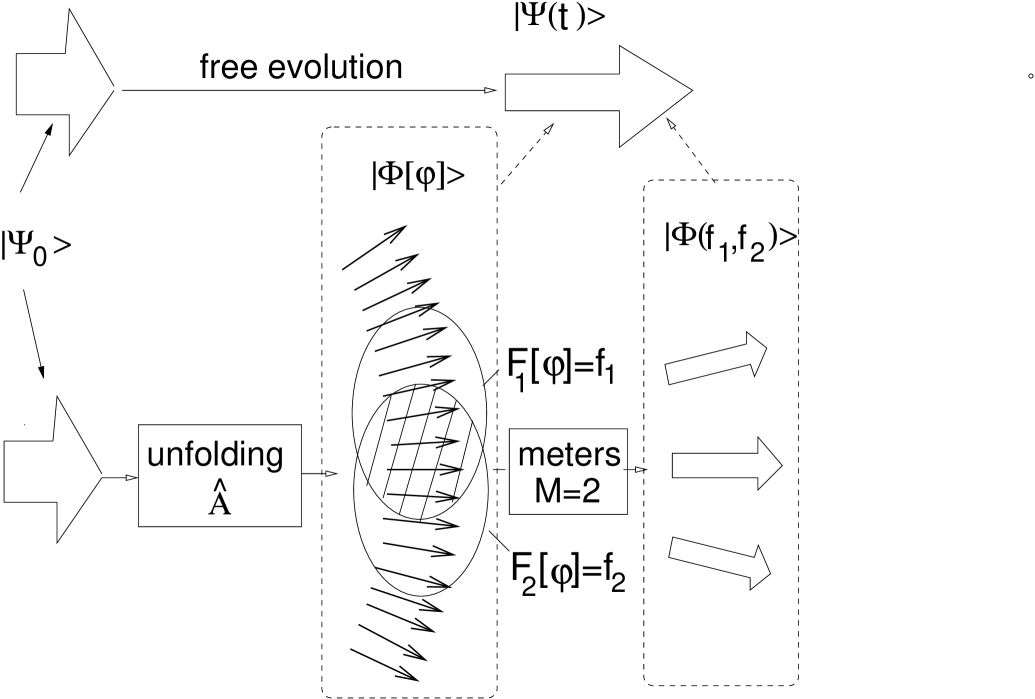
Figure 3: A system starts in a state $\Psi_{0}{\rangle}$ which, without measurements, would evolve into $\Psi(t){\rangle}$. $\Psi(t){\rangle}$ can be decomposed into a fine set of substates $|\Psi[\varphi]{\rangle}$, each labelled by a particular history $\varphi(t^{\prime})$. A meter decomposes $\Psi(t){\rangle}$ into a less informative substates, labelled by the value $f$ of functional $F[\varphi]$, which are obtained by summing $|\Psi[\varphi]>$ subject to restriction $F[\varphi]=f$. For the two meters shown, the substates in the shaded area are such that $F_{1}[\varphi]=f_{1}$ and $F_{2}[\varphi]=f_{2}$, and add up coherently to the state $|\Phi(f_{1}.f_{2}){\rangle}$, whose norm determines the probability to register both $f_{1}$ and $f_{2}$.

References

- (1) R.P. Feynman and A.R. Hibbs, Quantum Mechanics and Path Integrals (McGraw-Hill, New York 1965).
- (2) J. von Neumann, Mathematical Foundations of Quantum Mechanics (Princeton University Press, Princeton, 1955)
- (3) L.S. Schulman, Techniques and Applications of Path Integration (Wiley, New York, 1981), pp.225-236
- (4) H. Kleinert, Path Integrals in Quantum Mechanics, Statistics, Polymer Physics and Financial Markets Techniques and Applications of Path Integration (Wiley, New York, 1981), pp.225-236
- (5) M. Büttiker, Phys.Rev.B 27,6178 (1983)
- (6) R. Sala Mayato, D. Alonso and I.L. Egusquiza, in Time in Quantum Mechanics, edited by J.G. Muga, R. Sala Mayato and I.L. Eguisquiza (Springer, 2002)
- (7) N. Yamada, Prog.Theor.Phys. 83,985 (1991)
- (8) N. Yamada, Phys.Rev.A 54,182 (1996)
- (9) A. Peres and W.K. Wooters, Phys.Rev.D 32,1968 (1985)
- (10) D. Sokolovski and J.N.L Connor, Phys.Rev.A 44, 1500 (1991)
- (11) D. Sokolovski and J.N.L Connor, Phys.Rev.A 47, 4677 (1993).
- (12) D. Sokolovski and J.N.L Connor, Solid State Comm. 89, 475 (1994)
- (13) D. Sokolovski, S. Brouard and J.N.L Connor, Phys.Rev.A 50, 1240 (1994)
- (14) D. Sokolovski: Phys.Rev.A 52, R5 (1995)
- (15) D. Sokolovski: Phys.Rev.E 54, 1457 (1996)
- (16) D. Sokolovski: ’Path Integrals and the Quantum Traversal Time Problem’. In:Proceedinge of the Adriatico Research Conference on Tunnelling and its Implications, ed by D. Mugnai, A. Ranfagni and L.S. Schulman (World Scientific, Singapore New Jersey London New York, 1997), pp 206-222.
- (17) D. Sokolovski, Phys.Rev.Lett. 25, 4946 (1997)
- (18) D. Sokolovski, Phys.Rev.A 57, R1469 (1998)
- (19) D. Sokolovski, Phys.Rev.A 59, 1003 (1999)
- (20) D. Sokolovski and Y.Liu, Phys.Rev.A 63, 012109 (2000)
- (21) Y. Liu and D. Sokolovski, Phys.Rev.A 63, 014102 (2001)
- (22) D. Sokolovski, Proc.Royal.Soc.A, (2004) (in print)
- (23) D. Sokolovski, Phys.Rev.A 66, (2002)
- (24) D. Sokolovski, in Time in Quantum Mechanics, edited by J.G. Muga, R. Sala Mayato and I.L. Eguisquiza (Springer, 2002)
- (25) M.B. Mensky, Quantum Measurements and Path Integrals (IOP, Bristol,1993).
- (26) M.B. Mensky, Phys.Lett.A 196, 159 (1994)
- (27) M.B. Mensky, Phys.Lett.A 219, 137 (1996)
- (28) M.B. Mensky, Phys.Lett.A 231, 1(1997)
- (29) M.B. Mensky, Int.J.Theor.Phys 37, 273 (1998)
- (30) M.B. Mensky, Int.J.Theor.Phys 37, 215 (1998)
- (31) M.B. Mensky, Phys.Lett.A 307, 85 (2003)
- (32) M.B. Mensky, Phys.Lett.A 308, 243 (2003)
- (33) Y. Aharonov, D.Z. Albert and L. Vaidman, Phys. Rev. Lett. 60, 1351 (1988)
- (34) Y. Aharonov and L. Vaidman, in Time in Quantum Mechanics, edited by J.G. Muga, R. Sala Mayato and I.L. Eguisquiza (Springer, 2002), pp.369-413
- (35) Y. Aharonov and L. Vaidman, Phys.Rev.A 41, 11 (1990)
- (36) D. Sokolovski, Proc.Royal.Soc.A 460, 499 (2004)
- (37) D. Sokolovski, A.Z. Msezane and V.Shaginyan, quant-ph/0401159
- (38) R.P. Feynman, The Character of Physical Laws (Penguin, London, 1992)
- (39) ’Coarse graining’ may not be the most appropriate term as it usually implies separation of a set into a number of well defined non-overlapping subsets. In our case, the subsets of paths are fuzzy and overlapping. Yet, in the absence of a better word and to preserve the continuity with the previous work, we will continue to use it in this paper.
- (40) Messiah, Quantum Mechanics (North Holland, Amsterdam, 1961)
- (41) E. Arthurs and J.L. Kelly, Bell.Syst.Tech.J, 44, 725 (1965)
- (42) B. Bodmann, H. Leschke and S. Warzel, quant-ph/9703031